C. Jekeli, The Ohio State University, Columbus, OH, USA
ª2007 Elsevier B.V. All rights reserved.
3.02.1 Introduction 12
3.02.1.1 Historical Notes 12
3.02.1.2 Coordinate Systems 14
3.02.1.3 Preliminary Definitions and Concepts 14
3.02.2 Newton’s Law of Gravitation 15
3.02.3 Boundary-Value Problems 18
3.02.3.1 Green’s Identities 18
3.02.3.2 Uniqueness Theorems 20
3.02.3.3 Solutions by Integral Equation 21
3.02.4 Solutions to the Spherical BVP 22
3.02.4.1 Spherical Harmonics and Green’s Functions 22
3.02.4.2 Inverse Stokes and Hotine Integrals 25
3.02.4.3 Vening-Meinesz Integral and Its Inverse 26
3.02.4.4 Concluding Remarks 27
3.02.5 Low-Degree Harmonics: Interpretation and Reference 28
3.02.5.1 Low-Degree Harmonics as Density Moments 28
3.02.5.2 Normal Ellipsoidal Field 30
3.02.6 Methods of Determination 32
3.02.6.1 Measurement Systems and Techniques 33
3.02.6.2 Models 37
3.02.7 The Geoid and Heights 38
References 41
Glossary
deflection of the vertical Angle between direction of gravity and direction of normal gravity.
density moment Integral over the volume of a body of the product of its density and integer powers of Cartesian coordinates.
disturbing potential The difference between Earth’s gravity potential and the normal potential. eccentricity The ratio of the difference of squares of semimajor and semiminor axes to the square of the semimajor axis of an ellipsoid.
ellipsoid Surface formed by rotating an ellipse about its minor axis.
equipotential surface Surface of constant potential.
flattening The ratio of the difference between semimajor and semiminor axes to the semimajor axis of an ellipsoid.
geodetic reference system Normal ellipsoid with defined parameters adopted for general geodetic and gravimetric referencing.
geoid Surface of constant gravity potential that closely approximates mean sea level.
geoid undulation Vertical distance between the geoid and the normal ellipsoid, positive if the geoid is above the ellipsoid.
geopotential number Difference between gravity potential on the geoid and gravity potential at a point.
gravitation Attractive acceleration due to mass. gravitational potential Potential due to gravita-tional acceleration.
gravity Vector sum of gravitation and centrifugal acceleration due to Earth’s rotation.
gravity anomaly The difference between Earth’s gravity on the geoid and normal gravity on the
3.02.1
Introduction
Gravitational potential theory has its roots in the late Renaissance period when the position of the Earth in the cosmos was established on modern scientific (observation-based) grounds. A study of Earth’s grav-itational field is a study of Earth’s mass, its influence on near objects, and lately its redistributing transport in time. It is also fundamentally a geodetic study of Earth’s shape, described largely (70%) by the surface of the oceans. This initial section provides a historical backdrop to potential theory and introduces some concepts in physical geodesy that set the stage for later formulations.
3.02.1.1 Historical Notes
Gravitation is a physical phenomenon so pervasive and incidental that humankind generally has taken it for granted with scarcely a second thought. The Greek philosopher Aristotle (384–322 BC) allowed no more than to assert that gravitation is a natural property of material things that causes them to fall
(or rise, in the case of some gases), and the more material the greater the tendency to do so. It was enough of a self-evident explanation that it was not yet to receive the scrutiny of the scientific method, the beginnings of which, ironically, are credited to Aristotle. Almost 2000 years later, Galileo Galilei (1564–1642) finally took up the challenge to under-stand gravitation through observation and scientific investigation. His experimentally derived law of fall-ing bodies corrected the Aristotelian view and divorced the effect of gravitation from the mass of the falling object – all bodies fall with the same acceleration. This truly monumental contribution to physics was, however, only a local explanation of how bodies behaved under gravitational influence. Johannes Kepler’s (1571–1630) observations of pla-netary orbits pointed to other types of laws, principally an inverse-square law according to which bodies are attracted by forces that vary with the inverse square of distance. The genius of Issac Newton (1642–1727) brought it all together in his Philosophiae Naturalis Principia Mathematica of 1687 with a single and simple all-embracing law that in ellipsoid, either as a difference in vectors or a
dif-ference in magnitudes.
gravity disturbance The difference between Earth’s gravity and normal gravity, either as a dif-ference in vectors or a difdif-ference in magnitudes. gravity potential Potential due to gravity acceleration.
harmonic function Function that satisfies Laplace’s field equation.
linear eccentricity The distance from the center of an ellipsoid to either of its foci.
mean Earth ellipsoid Normal ellipsoid with para-meters closest to actual corresponding parapara-meters for the Earth.
mean tide geoid Geoid with all time-varying tidal effects removed.
multipoles Stokes coefficients.
Newtonian potential Harmonic function that approaches the potential of a point mass at infinity. non-tide geoid Mean tide geoid with all (direct and indirect deformation) mean tide effects removed.
normal ellipsoid Earth-approximating reference ellipsoid that generates a gravity field in which it is a surface of constant normal gravity potential.
normal gravity Gravity associated with the normal ellipsoid.
normal gravity potential Gravity potential asso-ciated with the normal ellipsoid.
orthometric height Distance along the plumb line from the geoid to a point.
potential Potential energy per unit mass due to the gravitational field; always positive and zero at infinity.
sectorial harmonics Surface spherical harmonics that do not change in sign with respect to latitude. Stokes coefficients Constants in a series expan-sion of the gravitational potential in terms of spherical harmonic functions.
surface spherical harmonics Basis functions defined on the unit sphere, comprising products of normalized associated Legendre functions and sinusoids.
tesseral harmonics Neither zonal nor sectorial harmonics.
zero-tide geoid Mean tide geoid with just the mean direct tidal effect removed (indirect effect due to Earth’s permanent deformation is retained). zonal harmonics Spherical harmonics that do not depend on longitude.
one bold stroke explained the dynamics of the entire universe (today there is more to understanding the dynamics of the cosmos, but Newton’s law remark-ably holds its own). The mass of a body was again an essential aspect, not as a self-attribute as Aristotle had implied, but as the source of attraction for other bodies: each material body attracts every other mate-rial body according to a very specific rule (Newton’s law of gravitation; see Section 3.02.2). Newton regretted that he could not explain exactly why mass has this property (as one still yearns to know today within the standard models of particle and quantum theories). Even Albert Einstein (1879– 1955) in developing his general theory of relativity (i.e., the theory of gravitation) could only improve on Newton’s theory by incorporating and explaining action at a distance (gravitational force acts with the speed of light as a fundamental tenet of the theory). What actually mediates the gravitational attraction still intensely occupies modern physicists and cosmologists.
Gravitation since its early scientific formulation initially belonged to the domain of astronomers, at least as far as the observable universe was concerned. Theory successfully predicted the observed perturba-tions of planetary orbits and even the location of previously unknown new planets (Neptune’s discov-ery in 1846 based on calculations motivated by observed perturbations in Uranus’ orbit was a major triumph for Newton’s law). However, it was also dis-covered that gravitational acceleration varies on Earth’s surface, with respect to altitude and latitude. Newton’s law of gravitation again provided the back-drop for the variations observed with pendulums. An early achievement for his theory came when he suc-cessfully predicted the polar flattening in Earth’s shape on the basis of hydrostatic equilibrium, which was confirmed finally (after some controversy) with geo-detic measurements of long triangulated arcs in 1736– 37 by Pierre de Maupertuis and Alexis Clairaut. Gravitation thus also played a dominant role in geo-desy, the science of determining the size and shape of the Earth, promulgated in large part by the father of modern geodesy, Friedrich R. Helmert (1843–1917).
Terrestrial gravitation through the twentieth cen-tury was considered a geodetic area of research, although, of course, its geophysical exploits should not be overlooked. But the advancement in modeling accuracy and global application was promoted mainly by geodesists who needed a well-defined reference for heights (a level surface) and whose astronomic observations of latitude and longitude
needed to be corrected for the irregular direction of gravitation. Today, the modern view of a height reference is changing to that of a geometric, mathe-matical surface (an ellipsoid) and three-dimensional coordinates (latitude, longitude, and height) of points on the Earth’s surface are readily obtained geometri-cally by ranging to the satellites of the Global Positioning System (GPS). The requirements of gravitation for GPS orbit determination within an Earth-centered coordinate system are now largely met with existing models. Improvements in gravita-tional models are motivated in geodesy primarily for rapid determination of traditional heights with respect to a level surface. These heights, for example, the orthometric heights, in this sense then become derived attributes of points, rather than their cardinal components.
Navigation and guidance exemplify a further spe-cific niche where gravitation continues to find important relevance. While GPS also dominates this field, the vehicles requiring completely autono-mous, self-contained systems must rely on inertial instruments (accelerometers and gyroscopes). These do not sense gravitation (see Section 3.02.6.1), yet gravitation contributes to the total definition of the vehicle trajectory, and thus the output of inertial navigation systems must be compensated for the effect of gravitation. By far the greatest emphasis in gravitation, however, has shifted to the Earth sciences, where detailed knowledge of the configura-tion of masses (the solid, liquid, and atmospheric components) and their transport and motion leads to improved understanding of the Earth systems (cli-mate, hydrologic cycle, tectonics) and their interactions with life. Oceanography, in particular, also requires a detailed knowledge of a level surface (the geoid) to model surface currents using satellite altimetry. Clearly, there is an essential temporal component in these studies, and, indeed, the tem-poral gravitational field holds center stage in many new investigations. Moreover, Earth’s dynamic beha-vior influences point coordinates and Earth-fixed coordinate frames, and we come back to fundamental geodetic concerns in which the gravitational field plays an essential role!
This section deals with the static gravitational field. The theory of the potential from the classical Newtonian standpoint provides the foundation for modeling the field and thus deserves the focus of the exposition. The temporal part is a natural exten-sion that is readily achieved with the addition of the time variable (no new laws are needed, if we neglect
general relativistic effects) and will not be expounded here. We are primarily concerned with gravitation on and external to the solid and liquid Earth since this is the domain of most applications. The internal field can also be modeled for specialized purposes (such as submarine navigation), but internal geophysical modeling, for example, is done usually in terms of the sources (mass density distribution), rather than the resulting field.
3.02.1.2 Coordinate Systems
Modeling the Earth’s gravitational field depends on the choice of coordinate system. Customarily, owing to the Earth’s general shape, a spherical polar coor-dinate system serves for most applications, and virtually all global models use these coordinates. However, the Earth is slightly flattened at the poles, and an ellipsoidal coordinate system has also been advocated for some near-Earth applications. We note that the geodetic coordinates associated with a geo-detic datum (based on an ellipsoid) are never used in a foundational sense to model the field since they do not admit to a separation-of-variables solution of Laplace’ differential equation (Section 3.02.4.1).
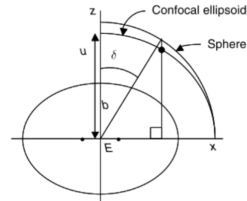
Spherical polar coordinates, described with the aid of Figure 1, comprise the spherical colatitude,
, the longitude,, and the radial distance, r. Their relation to Cartesian coordinates is
x ¼ r sincos
y ¼ r sinsin
z ¼ r cos
½1
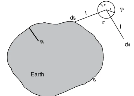
Considering Earth’s polar flattening, a better approximation, than a sphere, of its (ocean) surface is an ellipsoid of revolution. Such a surface is
generated by rotating an ellipse about its minor axis (polar axis). The two focal points of the best-fitting, Earth-centered ellipsoid (ellipse) are located in the equator about E¼522 km from the center of the Earth. A given ellipsoid, with specified semiminor axis, b, and linear eccentricity, E, defines the set of ellipsoidal coordinates, as described inFigure 2. The
longitude is the same as in the spherical case. The colatitude, , is the complement of the so-called reduced latitude; and the distance coordinate, u, is the semiminor axis of the confocal ellipsoid through the point in question. We call ð; ;uÞ ellipsoidal coordinates; they are also known as spheroidal coor-dinates, or Jacobi ellipsoidal coordinates. Their relation to Cartesian coordinates is given by
x¼pffiffiffiffiffiffiffiffiffiffiffiffiffiffiffiu2þE2sincos
y¼pffiffiffiffiffiffiffiffiffiffiffiffiffiffiffiu2þE2sinsin
z¼u cos
½2
Points on the given ellipsoid all have u¼b; and, all surfaces, u¼constant, are confocal ellipsoids (the analogy to the spherical case, when E¼0, should be evident).
3.02.1.3 Preliminary Definitions and Concepts
The gravitational potential, V, of the Earth is gener-ated by its total mass density distribution. For applications on the Earth’s surface it is useful to include the potential,, associated with the centrifu-gal acceleration due to Earth’s rotation. The sum, W ¼V þ, is then known, in geodetic terminology, as the gravity potential, distinct from gravitational potential. It is further advantageous to define a rela-tively simple reference potential, or normal potential, that accounts for the bulk of the gravity potential x y z r θ λ
Figure 1 Spherical polar coordinates.
x z E Confocal ellipsoid Sphere u b δ
(Section 3.02.5.2). The normal gravity potential, U, is defined as a gravity potential associated with a best-fitting ellipsoid, the normal ellipsoid, which rotates with the Earth and is also a surface of constant potential in this field. The difference between the actual and the normal gravity potentials is known as the disturbing potential: T ¼W–U ; it thus excludes the centrifugal potential. The normal gravity poten-tial accounts for approximately 99.999 5% of the total potential.
The gradient of the potential is an acceleration, gravity or gravitational acceleration, depending on whether or not it includes the centrifugal accelera-tion. Normal gravity, , comprises 99.995% of the total gravity, g, although the difference in magni-tudes, the gravity disturbance,dg, can be as large as several parts in 104. A special kind of difference, called the gravity anomaly, g, is defined as the difference between gravity at a point, P, and normal gravity at a corresponding point, Q, where WP¼UQ,
and P and Q are on the same perpendicular to the normal ellipsoid.
The surface of constant gravity potential, W0, that closely approximates mean sea level is known as the geoid. If the constant normal gravity potential, U0, on the normal ellipsoid is equal to the constant gravity potential of the geoid, then the gravity anomaly on the geoid is the difference between gravity on the geoid and normal gravity on the ellipsoid at respective points, P0, Q0, sharing the same perpendicular to the ellipsoid. The separation between the geoid and the ellipsoid is known as the geoid undulation, N, or also the geoid height (Figure 3). A simple Taylor expansion of the
normal gravity potential along the ellipsoid perpendi-cular yields the following important formula:
N¼T
½3
This is Bruns’ equation, which is accurate to a few millimeters in N, and which can be extended to N ¼T=–ðW0–U0Þ= for the general case,
W06¼U0. The gravity anomaly (on the geoid) is the gravity disturbance corrected for the evaluation of normal gravity on the ellipsoid instead of the geoid. This correction is Nq=qh ¼ ðq=qhÞðT=Þ, where h is height along the ellipsoid perpendicular. We haveg¼ –qT=qh, and hence
g¼ –qT qh þ 1 q qhT ½4
The slope of the geoid with respect to the ellip-soid is also the angle between the corresponding perpendiculars to these surfaces. This angle is known as the deflection of the vertical, that is, the deflection of the plumb line (perpendicular to the geoid) relative to the perpendicular to the normal ellipsoid. The deflection angle has components,,, respectively, in the north and east directions. The spherical approximations to the gravity disturbance, anomaly, and deflection of the vertical are given by
g ¼ –qT qr ; g ¼ – qT qr – 2 rT ¼ 1 qT rq; ¼ – 1 qT r sinq ½5
where the signs on the derivatives are a matter of convention.
3.02.2
Newton’s Law of Gravitation
In its original form, Newton’s law of gravitation applies only to idealized point masses. It describes the force of attraction, F, experienced by two suchsolitary masses as being proportional to the product of the masses, m1 and m2; inversely proportional to the distance,,, between them; and directed along the line joining them:
F ¼ Gm1m2
,2 n ½6
G is a constant, known as Newton’s gravitational constant, that takes care of the units between the left- and right-hand sides of the equation; it can be H, orthometric height Topographic surface Ellipsoid Geoid N, geoid undulation ellipsoidal height, h g Deflection of the vertical P0 Q0 W=W0 U=U0 P P0 Q0 Ellipsoidal height, h
determined by experiment and the current best value is (Groten, 2004):
G ¼ ð6:672590:00030Þ 10–11m3kg–1s–2 ½7 The unit vectorn in eqn [6] is directed from either
point mass to the other, and thus the gravitational force is attractive and applies equally to one mass as the other. Newton’s law of gravitation is universal as far as we know, requiring reformulation only in Einstein’s more comprehensive theory of general relativity which describes gravitation as a characteristic curva-ture of the space–time continuum (Newton’s formulation assumes instantaneous action and differs significantly from the general relativistic concept only when very large velocities or masses are involved).
We can ascribe a gravitational acceleration to the gravitational force, which represents the acceleration that one mass undergoes due to the gravitational attraction of the other. Specifically, from the law of gravitation, we have (for point masses) the gravita-tional acceleration of m1 due to the gravitational attraction of m2:
g ¼ Gm2
,2n ½8
The vectorg is independent of the mass, m1, of the body being accelerated (which Galileo found by experiment).
By the law of superposition, the gravitational force, or the gravitational acceleration, due to many point masses is the vector sum of the forces or accel-erations generated by the individual point masses. Manipulating vectors in this way is certainly feasible, but fortunately a more appropriate concept of grav-itation as a scalar field simplifies the treatment of arbitrary mass distributions.
This more modern view of gravitation (already adopted by Gauss (1777–1855) and Green (1793–1841)) holds that it is a field having a gravita-tional potential. Lagrange (1736–1813) fully developed the concept of a field, and the potential, V, of the gravitational field is defined in terms of the gravitational acceleration,g, that a test particle would
undergo in the field according to the equation
V ¼ g ½9
whereis the gradient operator (a vector). Further elucidation of gravitation as a field grew from Einstein’s attempt to incorporate gravitation into his special theory of relativity where no reference frame has special significance above all others. It was neces-sary to consider that gravitational force is not a real
force (i.e., it is not an applied force, like friction or propulsion) – rather, it is known as a kinematic force, that is, one whose action is proportional to the mass on which it acts (like the centrifugal force; see Martin, 1988). Under this precept, the geometry of space is defined intrinsically by the gravitational fields contained therein.
We continue with the classical Newtonian poten-tial, but interpret gravitation as an acceleration different from the acceleration induced by real, applied forces. This becomes especially important when considering the measurement of gravitation (Section 3.02.6.1). The gravitational potential, V, is a ‘scalar’ function, and, as defined here, V is derived directly on the basis of Newton’s law of gravitation. To make it completely consistent with this law and thus declare it a Newtonian potential, we must impose the following conditions:
lim
,!1,V ¼Gm and ,lim!1V ¼ 0 ½10 Here, m is the attracting mass, and we say that the potential is regular at infinity. It is easy to show that the gravitational potential at any point in space due to a point mass, in order to satisfy eqns [8]–[10], must be
V ¼ Gm
, ½11
where, again,,is the distance between the mass and the point at which the potential is expressed. Note that V for, ¼ 0 does not exist in this case; that is, the field of a point mass has a singularity. We use here the convention that the potential is always positive (in contrast to physics, where it is usually defined to be negative, conceptually closer to poten-tial energy).
Applying the law of superposition, the gravita-tional potential of many point masses is the sum of the potentials of the individual points (seeFigure 4):
VP ¼ G X j mj ,j ½12 And, for infinitely many points in a closed, bounded region with infinitesimally small masses, dm, the summation in eqn [12] changes to an integration,
VP ¼ G Z
mass dm
, ½13
or, changing variables (i.e., units), dm ¼ dv, where represents density (mass per volume) and dv is a volume element, we have (Figure 5)
VP ¼ G Z Z Z
volume,
dv ½14
In eqn [14],,is the distance between the evalua-tion point, P, and the point of integraevalua-tion. In spherical polar coordinates (Section 3.02.1.2), these points are ð; ;rÞ and ð9; 9;r9Þ, respectively. The volume element in this case is given by dv¼r92sin9d9d9dr9. V and its first derivatives are continuous everywhere – even in the case that P is on the bounding surface or inside the mass distribution, where there is the apparent singularity at, ¼ 0. In this case, by changing to a coordinate system whose origin is at P, the volume element becomes dv¼,2
sincddcd, (for some different colatitude and longitudecand); and, clearly, the singularity disappears – the integral is said to be weakly singular.
Suppose the density distribution over the volume depends only on radial distance (from the center of mass): ¼ ð Þr9, and that P is an exterior evaluation point. The surface bounding the masses necessarily is a sphere (say, of radius, R) and because of the
spherically symmetric density we may choose the integration coordinate system so that the polar axis passes through P. Then
,¼ pffiffiffiffiffiffiffiffiffiffiffiffiffiffiffiffiffiffiffiffiffiffiffiffiffiffiffiffiffiffiffiffiffiffiffiffiffiffiffiffir92þr2–2r9r cos9; d, ¼ 1
,r9r sin9d9
½15 It is easy to show that with this change of variables (fromto,) the integral [14] becomes simply
Vð; ;rÞ ¼ GM
r ; rR ½16
where M is the total mass bounded by the sphere. This shows that to a very good approximation the external gravitational potential of a planet such as the Earth (with concentrically layered density) is the same as that of a point mass.
Besides volumetric mass (density) distributions, it is of interest to consider surface distributions. Imagine an infinitesimally thin layer of mass on a surface, s, where the units of density in this case are those of mass per area. Then, analogous to eqn [14], the potential is
VP ¼ G Z Z
s ,
ds ½17
In this case, V is a continuous function everywhere, but its first derivatives are discontinuous at the sur-face. Or, one can imagine two infinitesimally close density layers (double layer, or layer of mass dipoles), where the units of density are now those of mass per area times length. It turns out that the potential in this case is given by (see Heiskanen and Moritz, 1967, p. 8) VP ¼ G Z Z s q qn 1 , ds ½18
where q=qn is the directional derivative along the perpendicular to the surface (Figure 5). Now, V itself
is discontinuous at the surface, as are all its derivatives. In all cases, V is a Newtonian potential, being derived from the basic formula [11] for a point mass that follows from Newton’s law of gravitation (eqn [6]).
The following properties of the gravitational potential are useful for subsequent expositions. First, consider Stokes’s theorem, for a vector func-tion,f, defined on a surface, s:
Z Z s r f ð Þ?n ds ¼ I p f?dr ½19 where p is any closed path in the surface, n is the unit vector perpendicular to the surface, and dr is a
l P n s dv ρ
Figure 5 Continuous density distribution. x y z m1 m2 m3 mj l1 l2 l3 lj P
Figure 4 Discrete set of mass points (superposition principle).
differential displacement along the path. From eqn [9], we find
r g¼ 0 ½20 since r r ¼ 0; hence, applying Stokes’s theo-rem, we find with F ¼ mg that
w ¼
I
F?ds ¼ 0 ½21 That is, the gravitational field is conservative: the work, w, expended in moving a mass around a closed path in this field vanishes. In contrast, dissipating forces (real forces!), like friction, expend work or energy, which shows again the special nature of the gravitational force.
It can be shown (Kellogg, 1953, p. 156) that the second partial derivatives of a Newtonian potential, V, satisfy the following differential equation, known as Poisson’s equation:
r2V ¼ –4G ½22 wherer2 ¼ ?formally is the scalar product of two gradient operators and is called the Laplacian operator. In Cartesian coordinates, it is given by
r2 ¼ q2 qx2þ q2 qy2þ q2 qz2 ½23 Note that the Laplacian is a scalar operator. Eqn [22] is a local characterization of the potential field, as opposed to the global characterization given by eqn [14]. Poisson’s equation holds wherever the mass den-sity, , satisfies certain conditions similar to continuity (Ho¨lder conditions; see Kellogg, 1953, pp. 152–153). A special case of eqn [22] applies for those points where the density vanishes (i.e., in free space); then Poisson’s equation turns into Laplace’ equation,
r2V ¼ 0 ½24 It is easily verified that the point mass potential satisfies eqn [24], that is,
r2 1 , ¼ 0 ½25 where, ¼ ffiffiffiffiffiffiffiffiffiffiffiffiffiffiffiffiffiffiffiffiffiffiffiffiffiffiffiffiffiffiffiffiffiffiffiffiffiffiffiffiffiffiffiffiffiffiffiffiffiffiffiffiffiffiffiffi x–x0 ð Þ2þðy–y0Þ2þðz–z0Þ2 q and the mass point is at xð 9;y9;z9Þ.
The solutions to Laplace’ equation [24] (that is, functions that satisfy Laplace’ equations) are known as harmonic functions (here, we also impose the conditions [10] on the solution, if it is a Newtonian potential and if the mass-free region includes infi-nity). Hence, every Newtonian potential is a
harmonic function in free space. The converse is also true: every harmonic function can be repre-sented as a Newtonian potential of a mass distribution (Section 3.02.3.1).
Whether as a volume or a layer density distribu-tion, the corresponding potential is the sum or integral of the source value multiplied by the inverse distance function (or its normal derivative for the dipole layer). This function depends on both the source points and the computation point and is known as a Green’s function. It is also known as the ‘kernel’ function of the integral representation of the potential. Functions of this type also play a dominant role in representing the potential as solutions to boundary-value problems (BVPs), as shown in sub-sequent sections.
3.02.3
Boundary-Value Problems
If the density distribution of the Earth’s interior and the boundary of the volume were known, then the problem of determining the Earth’s gravitational potential field is solved by the volume integral of eqn [14]. In reality, of course, we do not have access to this information, at least not the density, with sufficient detail. (The Preliminary Reference Earth Model (PREM), of Dziewonsky and Anderson (1981), still in use today by geophysicists, represents a good profile of Earth’s radial density, but does not attempt to model in detail the lateral density hetero-geneities.) In this section, we see how the problem of determining the exterior gravitational potential can be solved in terms of surface integrals, thus making exclusive use of accessible measurements on the surface.3.02.3.1 Green’s Identities
Formally, eqn [24] represents a partial differential equation for V. Solving this equation is the essence of the determination of the Earth’s external gravita-tional potential through potential theory. Like any differential equation, a complete solution is obtained only with the application of boundary conditions, that is, imposing values on the solution that it must assume at a boundary of the region in which it is valid. In our case, the boundary is the Earth’s surface and the exterior space is where eqn [24] holds (the atmosphere and other celestial bodies are neglected for the moment). In order to study the solutions to these BVPs (to show that solutions exist and are
unique), we take advantage of some very important theorems and identities. It is noted that only a rather elementary introduction to BVPs is offered here with no attempt to address the much larger field of solu-tions to partial differential equasolu-tions.
The first, seminal result is Gauss’ divergence the-orem (analogous to Stokes’ thethe-orem, eqn [19]),
Z Z Z v r?f dv ¼ Z Z s fnds ½26
wheref is an arbitrary (differentiable) vector
func-tion and fn¼n?f is the component of f along the
outward unit normal vector,n (see Figure 5). The
surface, s, encloses the volume, v. Equation [26] says that the sum of how muchf changes throughout the
volume, that is, the net effect, ultimately, is equiva-lent to the sum of its values projected orthogonally with respect to the surface. Conceptually, a volume integral thus can be replaced by a surface integral, which is important since the gravitational potential is due to a volume density distribution that we do not know, but we do have access to gravitational quan-tities on a surface by way of measurements.
Equation [26] applies to general vector functions that have continuous first derivatives. In particular, let U and V be two scalar functions having continuous second derivatives, and consider the vector function
f¼UV. Then, since n? ¼ q=qn, and
r?ðUrVÞ ¼ rU?rVþUr2V ½27 we can apply Gauss’ divergence theorem to get Green’s first identity,
Z Z Z v rU?rVþUr2V dv ¼ Z Z s UqV qn ds ½28
Interchanging the roles of U and V in eqn [28], one obtains a similar formula, which, when subtracted from eqn [28], yields Green’s second identity,
Z Z Z v Ur2V–Vr2U dv ¼ Z Z s UqV qn –V qU qn ds ½29 This is valid for any U and V with continuous deri-vatives up to second order.
Now let U ¼1=,, where, is the usual distance between an integration point and an evaluation point. And, suppose that the volume, v, is the space exterior to the Earth (i.e., Gauss’ divergence theorem applies to any volume, not just volumes containing a mass distribution). With reference to Figure 6, consider
the evaluation point, P, to be inside the volume (free
space) that is bounded by the surface, s; P is thus outside the Earth’s surface. Let V be a solution to eqn [24], that is, it is the gravitational potential of the Earth. From the volume, v, exclude the volume bounded by a small sphere, , centered at P. This sphere becomes part of the surface that bounds the volume, v. Then, since U, by our definition, is a point mass potential, r2U ¼0 everywhere in v (which excludes the interior of the small sphere around P); and, the second identity [29] gives
Z Z s 1 , qV qn –V q qn 1 , ds þ Z Z 1 , qV qn –V q qn 1 , d¼0 ½30 The unit vector, n, represents the perpendicular
pointing away from v. On the small sphere, n is opposite in direction to ,¼r , and the second inte-gral becomes Z Z –1 r qV qr þV q qr 1 r d¼ – Z Z 1 r qV qr r 2d – Z Z V d ¼ – Z Z qV qrr d–4V ½31 where d¼r2d,is the solid angle, 4, andV is an average value of V on. Now, in the limit as the radius of the small sphere shrinks to zero, the right-hand side of eqn [31] approaches 0–4VP. Hence,
eqn [30] becomes (Kellogg, 1953, p. 219)
VP¼ 1 4 Z Z s 1 , qV qn –V q qn 1 , ds ½32 dv l P σ s ds r l n l Earth n
Figure 6 Geometry for special case of Green’s third identity.
withn pointing down (away from the space outside
the Earth). This is a special case of Green’s third identity. A change in sign of the right-hand side transformsn to a normal unit vector pointing into v,
away from the masses, which conforms more to an Earth-centered coordinate system.
The right-hand side of eqn [32] is the sum of single- and double-layer potentials and thus shows that every harmonic function (i.e., a function that satisfies Laplace’ equation) can be written as a Newtonian potential. Equation [32] is also a solution to a BVP; in this case, the boundary values are inde-pendent values of V and of its normal derivative, both on s (Cauchy problem). Below and in Section 3.02.4.1, we encounter another BVP in which the potential and its normal derivative are given in a specified linear combination on s. Using a similar procedure and with some extra care, it can be shown (see also Courant and Hilbert, 1962, vol. II, p. 256 (footnote)) that if P is on the surface, then
VP¼ 1 2 Z Z s 1 , qV qn –V q qn 1 , ds ½33 where n points into the masses. Comparing this to eqn [32], we see that V is discontinuous as one approaches the surface; this is due to the double-layer part (see eqn [18]).
Equation [32] demonstrates that a solution to a particular BVP exists. Specifically, we are able to measure the potential (up to a constant) and its deri-vatives (the gravitational acceleration) on the surface and thus have a formula to compute the potential anywhere in exterior space, provided we also know the surface, s. Other BVPs also have solutions under appropriate conditions; a discussion of existence the-orems is beyond the present scope and may be found in (Kellogg, 1953). Equation [33] has deep geodetic significance. One objective of geodesy is to determine the shape of the Earth’s surface. If we have measure-ments of gravitational quantities on the Earth’s surface, then conceptually we are able to determine its shape from eqn [33], where it would be the only unknown quantity. This is the basis behind the work of Molodensky et al. (1962), to which we return briefly at the end of this section.
3.02.3.2 Uniqueness Theorems
Often the existence of a solution is proved simply by finding one (as illustrated above). Whether such as solution is the only one depends on a corresponding
uniqueness theorem. That is, we wish to know if a certain set of boundary values will yield just one potential in space. Before considering such theorems, we classify the BVPs that are typically encountered when determining the exterior potential from mea-surements on a boundary. In all cases, it is an exterior BVP; that is, the gravitational potential, V, is harmo-nic (r2V ¼0) in the space exterior to a closed surface that contains all the masses. The exterior space thus contains infinity. Interior BVPs can be constructed, as well, but are not applicable to our objectives.
•
Dirichlet problem (or, BVP of the first kind ). Solve for V in the exterior space, given its values every-where on the boundary.•
Neumann problem (or, BVP of the second kind ). Solve for V in the exterior space, given values of its normal derivative everywhere on the boundary.•
Robin problem (mixed BVP, or BVP of the third kind ). Solve for V in the exterior space, given a linear combination of it and its normal derivative on the boundary.Using Green’s identities, we prove the following theorems for these exterior problems; similar results hold for the interior problems.
Theorem 1. If V is harmonic (hence continuously differentiable) in a closed region, v, and if V vanishes everywhere on the boundary, s, then V also vanishes everywhere in the region, v.
Proof. Since V ¼0 on s, Green’s first identity (eqn [28]) with U ¼V gives Z Z Z rV ð Þ2dv¼ Z Z s VqV qnds¼0 ½34
The integral on the left side is therefore always zero, and the integrand is always non-negative. Hence, V ¼0 everywhere in v, which implies
that V ¼constant in v. Since V is continuous in v and V ¼0 on s, that constant must be zero; and so V ¼0 in v.
This theorem solves the Dirichlet problem for the trivial case of zero boundary values and it enables the following uniqueness theorem for the general Dirichlet problem.
Theorem 2 (Stokes’ theorem). If V is harmonic (hence continuously differentiable) in a closed region, v, then V is uniquely determined in v by its values on the boundary, s.
Proof. Suppose the determination is not unique: that is, suppose there are V1 and V2, both harmonic
in v and both having the same boundary values on s. Then the function V ¼V2–V1is harmonic in v with all boundary values equal to zero. Hence, by Theorem 1, V2–V1¼0 identically in v, or V2¼V1 everywhere, which implies that any determination is unique based on the boundary values.
Theorem 3. If V is harmonic (hence continuously differentiable) in the exterior region, v, with closed boundary, s, then V is uniquely determined by the values of its normal derivative on s.
Proof. We begin with Green’s first identity, eqn [28], as in the proof of Theorem 1 to show that if the normal derivative vanishes everywhere on s, then V is a constant in v. Now, suppose there are two harmonic functions in v: V1 and V2, with the same normal derivative values on s. Then the normal derivative values of their difference are zero; and, by the above demonstration, V ¼V2–V1¼constant in v. Since V is a Newtonian potential in the exterior space, that constant is zero, since by eqn [10], lim,!1V ¼0. Thus, V2¼V1, and the boundary values determine the potential uniquely.
This is a uniqueness theorem for the exterior Neumann BVP. Solutions to the interior problem are unique only up to an arbitrary constant.
Theorem 4. Suppose V is harmonic (hence continu-ously differentiable) in the closed region, v, with boundary, s; and, suppose the boundary values are given by g¼VjsþqV qn s ½35
Then V is uniquely determined by these values if = >0.
Proof. Suppose there are two harmonic functions, V1 and V2, with the same boundary values, g, on s. Then V ¼V2–V1is harmonic with boundary values
ðV2–V1Þjsþ qV2 qn – qV1 qn s¼0 ½36
With U ¼V ¼V2–V1, Green’s first identity, eqn [28], gives Z Z Z v rðV2–V1Þ ð Þ2dv¼ Z Z s V2–V1 ð Þ– ðV2–V1Þds ½37 Then Z Z Z rðV2–V1Þ ð Þ2dvþ Z Z s V2–V1 ð Þ2dS¼0 ½38 Since= >0, eqn [38] implies thatrðV2–V1Þ ¼0 in v; and V2–V1¼0 on s. Hence V2–V1¼constant
in v; and V2¼V1on s. By the continuity of V1and V2, the constant must be zero, and the uniqueness is proved.
The solution to the Robin problem is unique only in certain cases. The most famous problem in physi-cal geodesy is the determination of the disturbing potential, T, from gravity anomalies, g, on the geoid (Section 3.02.1.3). Suppose T is harmonic out-side the geoid; the second of eqns [5] provides an approximate form of boundary condition, showing that this is a type of Robin problem. We find that ¼ –2=r , and, recalling that when v is the exterior space the unit vector n points inward toward the masses, that is,q=qn¼ –q=qr , we get ¼1. Thus, the condition in Theorem 4 on= is not fulfilled and the uniqueness is not guaranteed. In fact, we will see that the solution obtained for the spherical boundary is arbitrary with respect to the coordinate origin (Section 3.02.4.1).
3.02.3.3 Solutions by Integral Equation Green’s identities show how a solution to Laplace’s equation can be transformed from a volume integral, that is, an integral of source points, to a surface integral of BVPs, as demonstrated by eqn [32]. The uniqueness theorems for the BVPs suggest that the potential due to a volume density distribution can also be represented as due to a generalized density layer on the bounding surface, as long as the result is harmonic in exterior space, satisfies the boundary conditions, and is regular at infinity like a Newtonian potential. Molodensky et al. (1962) sup-posed that the disturbing potential is expressible as
T¼
Z Z s
,ds ½39
where is a surface density to be solved using the boundary condition. With the spherical approxima-tion for the gravity anomaly, eqn [5], one arrives at the following integral equation
2cos– Z Z s q qr 1 , þ 2 r, ds¼g ½40 The first term accounts for the discontinuity at the surface of the derivative of the potential of a density layer, where is the deflection angle between the normal to the surface and the direction of the (radial) derivative (Heiskanen and Moritz, 1967, p. 6; Gu¨nter, 1967, p. 69). This Fredholm integral equation of the second kind can be simplified with further approx-imations, and, a solution for the density,, ultimately
leads to the solution for the disturbing potential (Moritz, 1980).
Other forms of the initial representation have also been investigated, where Green’s functions other than 1=,lead to simplifications of the integral equa-tion (e.g., Petrovskaya, 1979). Nevertheless, most practical solutions rely on approximations, such as the spherical approximation for the boundary condi-tion, and even the formulated solutions are not strictly guaranteed to converge to the true solutions (Moritz, 1980). Further treatments of the BVP in a geodetic/mathematical setting may be found in the volume edited by Sanso` and Rummel (1997).
In the next section, we consider solutions for T as surface integrals of boundary values with appropriate Green’s functions. In other words, the boundary values (whether of the first, second, or third kind) may be thought of as sources, and the consequent potential is again the sum (integral) of the product of a boundary value and an appropriate Green’s func-tion (i.e., a funcfunc-tion that depends on both the source point and the computation point in some form of inverse distance in accordance with Newtonian potential theory). Such solutions are readily obtained if the boundary is a sphere.
3.02.4
Solutions to the Spherical BVP
This section develops two types of solutions to stan-dard BVPs when the boundary is a sphere: the spherical harmonic series and an integral with a Green’s function. All three types of problems are solved, but emphasis is put on the third BVP since gravity anomalies are the most prevalent boundary values (on land, at least). In addition, it is shown how the Green’s function integrals can be inverted to obtain, for example, gravity anomalies from values of the potential, now considered as boundary values. Not all possible inverse relationships are given, but it should be clear at the end that, in principle, virtually any gravitational quantity can be obtained in space from any other quantity on the spherical boundary. 3.02.4.1 Spherical Harmonics and Green’s FunctionsFor simple boundaries, Laplace’s equation [24] is rela-tively easy to solve provided there is an appropriate coordinate system. For the Earth, the solutions com-monly rely on approximating the boundary by a sphere. This case is described in detail and a more accurate
approximation based on an ellipsoid of revolution is briefly examined in Section 3.02.5.2 for the normal potential. In spherical polar coordinates,ð; ;rÞ, the Laplacian operator is given by Hobson (1965, p. 9)
r2¼ 1 r2 q qr r 2 q qr þ 1 r2 1 sin q q sin q q þ 1 r2sin2 q2 q2 ½41
A solution tor2V ¼0 in the space outside a sphere of radius, R, with center at the coordinate origin can be found by the method of separation of variables, whereby one postulates the form of the solution, V, as
Vð; ;rÞ ¼fð Þ gð Þh rð Þ ½42 Substituting this and the Laplacian above into eqn [24], the multivariate partial differential equation separates into three univariate ordinary differential equations (Hobson, 1965, p. 9; Morse and Feshbach, 1953, p. 1264). Their solutions are well-known func-tions, for example,
Vð; ;rÞ ¼PnmðcosÞsin m 1 rnþ1 ½43a or Vð; ;rÞ ¼PnmðcosÞcos m 1 rnþ1 ½43b where Pnmð Þt is the associated Legendre function of
the first kind and n, m are integers such that 0mn, n0. Other solutions are also possible (e.g., gð Þ ¼ ea
aPR
ð Þ and hðrÞ ¼rn), but only
eqns [43] are consistent with the problem at hand: to find a real-valued Newtonian potential for the exterior space of the Earth (regular at infinity and 2-periodic in longitude). The general solution is a linear combination of solutions of the forms given by eqns [43] for all possible integers, n and m, and can be written compactly as Vð; ;rÞ ¼X 1 n¼0 Xn m¼–n R r nþ1 vnmYnmð; Þ ½44
where theYnm are surface spherical harmonic
func-tions defined as Ynmð; Þ ¼Pn mj jðcosÞ cos m; m0 sin mj j; m<0 ( ½45
andPnm is a normalization of Pnm so that the
1 4 Z Z Ynmð; ÞYn9m9ð; Þd ¼ 1; n¼n9 and m¼m9 0; n6¼n9 or m6¼m9 ( ½46 and where ¼fð; Þj0; 02g represents the unit sphere, with d¼ sindd. For a complete mathematical treatment of spheri-cal harmonics, one may refer to Mu¨ller (1966). The bounding spherical radius, R, is introduced so that all the constant coefficients, vnm, also known as
Stokes constants, have identical units of measure. Applying the orthogonality to the general solution [44], these coefficients can be determined if the function, V, is known on the bounding sphere (boundary condition): vnm¼ 1 4 Z Z Vð; ;RÞYnmð; Þd ½47 Equation [44] is known as a spherical harmonic expansion of V and with eqn [47] it represents a solution to the Dirichlet BVP if the boundary is a sphere. The solution thus exists and is unique in the sense that these boundary values generate no other potential. We will, however, find another equivalent form of the solution.
In a more formal mathematical setting, the solution [46] is an infinite linear combination of orthogonal basis functions (eigenfunctions) and the coefficients, vnm, are
the corresponding eigenvalues. One may also interpret the set of coefficients as the spectrum (Legendre spec-trum) of the potential on the sphere of radius, R (analogous to the Fourier spectrum of a function on the plane or line). The integers, n, m, correspond to wave numbers, and are called degree (n) and order (m), respectively. The spherical harmonics are further clas-sified as zonal (m¼0), meaning that the zeros ofYn0
divide the sphere into latitudinal zones; sectorial (m¼n), where the zeros ofYnndivide the sphere into
longitudinal sectors; and tesseral (the zeros ofYnm
tes-sellate the sphere) (Figure 7).
While the spherical harmonic series has its advantages in global representations and spectral inter-pretations of the field, a Green’s function representation provides a more local characterization of the field. Changing a boundary value anywhere on the globe changes all coefficients, vnm, according to eqn [47],
which poses both a numerical challenge in applications, as well as in keeping a standard model up to date. However, since the Green’s function essentially depends on the inverse distance (or higher power thereof), a remote change in boundary value generally does not appreciably affect the local determination of the field.
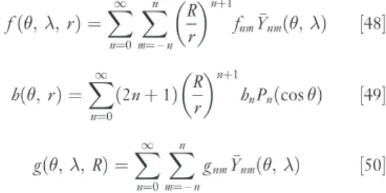
When the boundary is a sphere, the solutions to the BVPs using a Green’s function are easily derived from the spherical harmonic series representation. Moreover, it is possible to derive additional integral relationships (with appropriate Green’s functions) among all the derivatives of the potential. To forma-lize and simultaneously simplify these derivations, consider harmonic functions, f and h, where h depends only onand r, and function g, defined on the sphere of radius, R. Thus let
fð; ;rÞ ¼X 1 n¼0 Xn m¼–n R r nþ1 fnmYnmð; Þ ½48 hð;rÞ ¼X 1 n¼0 2nþ1 ð Þ R r nþ1 hnPnðcosÞ ½49 gð; ;RÞ ¼X 1 n¼0 Xn m¼–n gnmYnmð; Þ ½50 where PnðcosÞ ¼Pn0ðcosÞ= ffiffiffiffiffiffiffiffiffiffiffiffiffi2nþ1
p
is the nth degree Legendre polynomial. Constants fnm and gnm
are the respective harmonic coefficients of f and g when these functions are restricted to the sphere of radius, R. Then, using the decomposition formula for Legendre polynomials,
P87 (cosθ) cos7λ
P88 (cosθ) cos8λ
P80 (cosθ)
PnðcoscÞ ¼ 1 2nþ1 Xn m¼–n Ynmð; ÞYnmð9; 9Þ ½51 where
cosc¼coscos9þsinsin9cosð–9Þ ½52 it is easy to prove the following theorem.
Theorem (convolution theorem in spectral analysis on the sphere). fð; ;rÞ ¼ 1 4 Z Z gð9; 9;RÞhðc;rÞd if and only if fnm¼gnmhn ½53
Here, and in the following, d¼ sin9d9d9. The angle,c, is the distance on the unit sphere between pointsð; Þandð9; 9Þ.
Proof. The forward statement [53] follows directly by substituting eqns [51] and [49] into the first equation [53], together with the spherical harmonic expansion [50] for g. A comparison with the spherical harmonic expansion for f yields the result. All steps in this proof are reversible, and so the reverse statement also holds.
Consider now f to be the potential, V, outside the sphere of radius, R, and its restriction to the sphere to be the function, g:gð; Þ ¼Vð; ;RÞ. Then, clearly, hn¼1, for all n; by the theorem above, we have
Vð; ;rÞ ¼ 1 4 Z Z Vð9; 9;RÞUðc;rÞd ½54 where Uðc;rÞ ¼X 1 n¼0 2nþ1 ð Þ R r nþ1 PnðcoscÞ ½55
For the distance
,¼pffiffiffiffiffiffiffiffiffiffiffiffiffiffiffiffiffiffiffiffiffiffiffiffiffiffiffiffiffiffiffiffiffiffiffiffir2þR2–2rR cosc ½56 between pointsð; ;rÞandð9; 9;RÞ, with rR, the identity (the Coulomb expansion; Cushing, 1975, p. 155), 1 ,¼ 1 R X1 n¼0 R r nþ1 PnðcoscÞ ½57
yields, after some arithmetic (based on taking the derivative on both sides with respect to r),
Uðc;rÞ ¼R r 2–R2 ð Þ
,3 ½58
Solutions [44] and [54] to the Dirichlet BVP for a spherical boundary are identical (in view of the con-volution theorem [53]). The integral in [54] is known as the Poisson integral and the function U is the
corresponding Green’s function, also known as Poisson’s kernel.
For convenience, one separates Earth’s gravita-tional potential into a reference potential (Section 3.02.1.3) and the disturbing potential, T. The disturb-ing potential is harmonic in free space and satisfies the Poisson integral if the boundary is a sphere. In deference to physical geodesy where relationships between the disturbing potential and its derivatives are routinely applied, the following derivations are developed in terms of T, but hold equally for any exterior Newtonian potential. Let
Tð; ;rÞ ¼GM R X1 n¼0 Xn m¼–n R r nþ1 CnmYnmð; Þ ½59 where M is the total mass (including the atmosphere) of the Earth and the dCnm are unitless harmonic
coefficients, being also the difference between coeffi-cients for the total and reference gravitational potentials (Section 3.02.5.2). The coefficient,C00, is zero under the assumption that the reference field accounts completely for the central part of the total field. Also note that these coefficients specifically refer to the sphere of radius, R.
The gravity disturbance is defined (in spherical approximation) to be the negative radial derivative of T, the first of eqns [5]. From eqn [59], we have
gð; ;rÞ ¼ – q qrTð; ;rÞ ¼GM R2 X1 n¼0 Xn m¼–n R r nþ2 nþ1 ð ÞCnmYnmð; Þ ½60 and, applying the convolution theorem [53], we obtain Tð; ;rÞ ¼ R 4 Z Z gð9; 9;RÞHðc;rÞd ½61
where with gnm¼ðnþ1ÞdCnm=R and fnm¼dCnm, we
have hn¼fnm=gnm¼R=ðnþ1Þ, and hence (taking
care to keep the Green’s function unitless)
Hðc;rÞ ¼X 1 n¼0 2nþ1 nþ1 R r nþ1 PnðcoscÞ ½62
The integral in [61] is known as the Hotine integral, the Green’s function, H, is called the Hotine kernel, and with a derivation based on equation [57], it is given by (Hotine 1969, p. 311) Hðc;rÞ ¼2R , –ln 1þ , 2R sin2c=2 ½63
Equation [61] solves the Neumann BVP when the boundary is a sphere.
The gravity anomaly (again, in spherical approx-imation) is defined by eqn [5]
gð; ;rÞ ¼ – q qr – 2 r Tð; ;rÞ ½64 or, also, gð; ;rÞ ¼GM R2 X1 n¼0 Xn m¼–n R r nþ2 n–1 ð ÞCnmYnmð; Þ ½65 In this case, we have gnm ¼ðn–1ÞdCnm=R and
hn¼R=ðn–1Þ. The convolution theorem in this
case leads to the geodetically famous Stokes integral,
Tð; ;rÞ ¼ R 4
Z Z
gð9; 9;RÞSðc;rÞd ½66
where we define Green’s function to be
Sðc;rÞ ¼X 1 n¼2 2nþ1 n–1 R r nþ1 PnðcoscÞ ¼2R ,þ R r –3 R, r2 –5 R2 r2cosc –3R 2 r2coscln ,þr–R cosc 2r ½67
more commonly called the Stokes kernel. Equation [66] solves the Robin BVP if the boundary is a sphere, but it includes specific constraints that ensure the solution’s uniqueness – the solution by itself is not unique, in this case, as proved in Section 3.02.3.2. Indeed, eqn [65] shows that the gravity anomaly has no first-degree harmonics for the disturbing poten-tial; therefore, they cannot be determined from the boundary values. Conventionally, the Stokes kernel also excludes the zero-degree harmonic, and thus the complete solution for the disturbing potential is given by Tð; ;rÞ ¼GM r C00 þGM R X1 m¼–1 R r 2 C1mY1mð; Þ þ R 4 Z Z gð9; 9;RÞSðc;rÞd ½68
The central term,C00, is proportional to the differ-ence in GM of the Earth and referdiffer-ence ellipsoid and is zero to high accuracy. The first-degree harmonic coefficients,C1m, are proportional to the center-of-mass coordinates and can also be set to zero with appropriate definition of the coordinate system (see Section 3.02.5.1). Thus, the Stokes integral [66] is the
more common expression for the disturbing poten-tial, but it embodies hidden constraints.
We note that gravity anomalies also serve as boundary values in the harmonic series form of the solution for the disturbing potential. Applying the orthogonality of the spherical harmonics to eqn [65] yields immediately Cnm¼ R2 4ðn–1ÞGM Z Z gð9; 9;RÞYnmð9; 9Þd; n2 ½69
A similar formula holds when gravity disturbances are the boundary values (n–1 in the denominator changes to nþ1). In either case, the boundary values formally are assumed to reside on a sphere of radius, R. An approximation results if they are given on the geoid, as is usually the case.
3.02.4.2 Inverse Stokes and Hotine Integrals
The convolution integrals above can easily be inverted by considering again the spectral relationships. For the gravity anomaly, we note that f ¼rg is harmonic with coefficients, fnm ¼GM nð –1ÞdCnm=R. Letting gnm ¼GM dCnm=R,
we find that hn¼n–1; from the convolution
theo-rem, we can write gð; ;rÞ ¼ 1 4R Z Z Tð9; 9;RÞZˆðc;rÞd ½70 where ˆ Zðc;rÞ ¼X 1 n¼0 2nþ1 ð Þðn–1Þ R r nþ2 PnðcoscÞ ½71
The zero- and first-degree terms are included provi-sionally. Note that
ˆ Zðc;rÞ ¼ –R q qrþ 2 r Uðc;rÞ ½72
that is, we could have simply used the Dirichlet solution [54] to obtain the gravity anomaly, as given by [70], from the disturbing potential. It is convenient to separate the kernel function as follows:
ˆ Zðc;rÞ ¼Zðc;rÞ–X 1 n¼0 2nþ1 ð Þ R r nþ2 PnðcoscÞ ½73 where Zðc;rÞ ¼X 1 n¼1 2nþ1 ð Þn R r nþ2 PnðcoscÞ ½74
We find that gð; ;rÞ ¼ –1 rTð; ;rÞ þ 1 4R Z Z Tð9; 9;RÞZðc;rÞd ½75
Now, since Z has no zero-degree harmonics, its inte-gral over the sphere vanishes, and one can write the numerically more convenient formula:
gð; ;rÞ ¼–1 rTð; ;rÞ þ 1 4R Z Z ðTð9; 9;RÞ –Tð; ;RÞÞZðc;rÞd ½76
This is the inverse Stokes formula. Given T on the sphere of radius R (e.g., in the form of geoid undula-tions, T ¼N ), this form is useful when the gravity anomaly is also desired on this sphere. It is one way to determine gravity anomalies on the ocean surface from satellite altimetry, where the ocean surface is approximated as a sphere. Analogously, from eqns [60] and [64], it is readily seen that the inverse Hotine formula is given by
gð; ;rÞ ¼1 rTð; ;rÞ þ 1 4R Z Z ðTð9; 9;RÞ –Tð; ;RÞÞZðc;rÞd ½77 Note that the difference of eqns [76] and [77] yields the approximate relationship between the gravity disturbance and the gravity anomaly inferred from eqns [5].
Finally, we realize that, for r¼R, the series for Z c;R
ð Þ is not uniformly convergent and special numerical procedures (that are outside the present scope) are required to approximate the correspond-ing integrals.
3.02.4.3 Vening-Meinesz Integral and Its Inverse
Other derivatives of the disturbing potential may also be determined from boundary values. We consider here only gravity anomalies, being the most preva-lent data type on land areas. The solution is either in the form of a series – simply the derivative of the series [59] with coefficients given by eqn [69], or an integral with appropriate derivative of the Green’s function. The horizontal derivatives of the disturbing potential are often interpreted as the deflections of the vertical to which they are proportional in sphe-rical approximation (eqn [5]):
; ;ð rÞ ; ;ð rÞ ( ) ¼ 1 ;ð rÞ 1 r q q – 1 r sin q q 8 > > < > > : 9 > > = > > ; Tð; ;rÞ ½78 where; are the north and east deflection compo-nents, respectively, and is the normal gravity. Clearly, the derivatives can be taken directly inside the Stokes integral, and we find
; ;ð rÞ ; ;ð rÞ ( ) ¼ R 4r ;ð rÞ Z Z gð9; 9;RÞ q qcSðc;rÞ cos sin ( ) d ½79 where 1 r q q – 1 r sin q q 8 > > < > > : 9 > > = > > ; ¼1 r qc q – 1 sin qc q 8 > > < > > : 9 > > = > > ; q qc ½80 and qc q ¼ 1
sincðsincos9–cossin9cosð9–ÞÞ ¼cos
– 1 sin
qc q¼
1
sincsin9sinð9–Þ ¼ sin ½81
The angle,, is the azimuth ofð9; 9Þatð; Þon the unit sphere. The integrals [79] are known as the Vening-Meinesz integrals. Analogous integrals for the deflections arise when the boundary values are the gravity disturbances (the Green’s functions are then derivatives of the Hotine kernel).
For the inverse Vening-Meinesz integrals, we need to make use of Green’s first identity for surface functions, f and g: Z Z s fð Þg dsþ Z Z s rf ?rg ds¼ Z b f rg?n db ½82 where b is the boundary (a line) of surface, s;rand are the gradient and Laplace–Beltrami operators, which for the spherical surface are given by
r ¼ q q 1 sin q q 0 B B @ 1 C C A; ¼ q2 q2þcot q qþ 1 sin2 q2 q2 ½83
and where n is the unit vector normal to b. For a
closed surface such as the sphere, the line integral vanishes, and we have
Z Z fð Þg d¼ – Z Z rf ?rg d ½84 The surface spherical harmonics, Ynmð; Þ, satisfy
the following differential equation:
Ynmð; Þ þn nð þ1ÞYnmð; Þ ¼0 ½85 Therefore, the harmonic coefficients of T
; ;r
ð Þon the sphere of radius, R, are Tð; ;rÞ
½ nm¼ –n nð þ1ÞGM
R Cnm ½86
Hence, by the convolution theorem (again, consider-ing the harmonic function, f ¼rg),
gð; ;rÞ ¼ – 1 4R Z Z Tð9; 9;RÞWðc;rÞd ½87 where Wðc;rÞ ¼X 1 n¼2 2nþ1 ð Þðn–1Þ n nð þ1Þ R r nþ2 PnðcoscÞ ½88
and where the zero-degree term of the gravity anom-aly must be treated separately (e.g., it is set to zero in this case). Using Green’s identity [84] and eqns [80] and [81], we have gð; ;rÞ ¼ 1 4R Z Z rTð9; 9;RÞ?rWðc;rÞd ¼R0 4R Z Z ð ð 9; 9;RÞcos þ ð 9; 9;RÞsinÞ q qcWðc;rÞd ½89
where normal gravity on the sphere of radius, R, is approximated as a constant: ;ð RÞ.0. Equation [89] represents a second way to compute gravity anomalies from satellite altimetry, where the along-track and cross-track altimetric differences are used to approximate the deflection components (with appropriate rotation to north and east components). Employing differences in altimetric measurements benefits the estimation since systema-tic errors, such as orbit error, cancel out. To speed up the computations, the problem is reformulated in the spectral domain (see, e.g., Sandwell and Smith, 1996).
Clearly, following the same procedure for f ¼T , we also have the following relationship:
Tð; ;rÞ ¼R0 4 Z Z ð ð 9; 9;RÞcos þ ð 9; 9;RÞsinÞ q qcBðc;rÞd ½90 where Bðc;rÞ ¼X 1 n¼2 2nþ1 ð Þ n nð þ1Þ R r nþ1 PnðcoscÞ ½91
It is interesting to note that instead of an integral over the sphere, the inverse relationship between the dis-turbing potential on the sphere and the deflection of the vertical on the same sphere is also more straight-forward in terms of a line integral:
Tð; ;RÞ ¼Tð0; 0;RÞ þ 0 4 Z ð; Þ ð0;0Þ ð ð 9; 9;RÞds – ð 9; 9;RÞdsÞ ½92 where ds¼R d; ds¼R sin d ½93 3.02.4.4 Concluding Remarks
The spherical harmonic series, [59], represents the general solution to the exterior potential, regardless of the way the coefficients are determined. We know how to compute those coefficients exactly on the basis of a BVP, if the boundary is a sphere. More complicated boundaries would require corrections or, if these are omitted, would imply an approxima-tion. If the coefficients are determined accurately (e.g., from satellite observations (Section 3.02.6.1), but not according to eqn [69]), then the spherical harmonic series model for the potential is not a spherical approximation. The spherical approxima-tion enters when approximate relaapproxima-tions such as eqns [5] are used and when the boundary is approximated as a sphere. However determined, the infinite series converges uniformly for all r >Rc, where Rc is the
radius of the sphere that encloses all terrestrial masses. It may also converge below this sphere, but would represent the true potential only in free space (above the Earth’s surface, where Laplace’s equation holds). In practice, though, convergence is not an