Experimental Study of Second-Mode Instabilities on a
7-Degree Cone at Mach 6
Shann J. Rufer1
NASA Langley Research Center, Hampton, VA, 23681 Dennis C. Berridge2
School of Aeronautics and Astronautics, Purdue University, West Lafayette, IN, 47907 NASA Langley Research Center, Hampton, VA, 23681
Experiments have been carried out in the NASA Langley Research Center 20-Inch Mach 6 Air Tunnel to measure the second-mode boundary-layer instability on a 7° half-angle cone using high-frequency pressure sensors. Data were obtained with both blunt and sharp nosetips installed on the cone. The second-mode wave amplitudes were observed to saturate and then begin to decrease in the Langley tunnels, indicating wave breakdown. Pressure fluctuation measurements and thermocouple data indicated the location of transition along the cone at the different conditions tested. Comparisons between the power density spectra obtained during the current test and previous data from the Langley 15-Inch Mach 6 High Temperature Tunnel and the Boeing/AFOSR Mach 6 Quiet tunnel illustrate the effect of tunnel noise on instability growth and transition.
Nomenclature
A disturbance amplitude A0 initial disturbance amplitude
D diameter (m) f frequency (kHz) M Mach number
N integrated amplification factor P, p pressure (kPa)
Re Reynolds number St Stanton number T temperature (K) t time (seconds)
x cone axial coordinate (m)
φ cone azimuthal coordinate (degrees) Superscript
′ fluctuations
Subscript
0 stagnation condition mean average (mean) w wall condition
θ momentum thickness e edge
Abbreviations
AoA Angle of Attack
AEDC Arnold Engineering Development Center LaRC NASA Langley Research Center
PSD Power Spectral Density RMS Root Mean Square
STABL Stability and Transition for hypersonic Boundary Layers
t,1 reservoir stagnation
_______________
1 Aerospace Engineer, Aerothermodynamics Branch, AIAA Senior Member. 2 Research Assistant and Co-op Student, AIAA Student Member
I.
Introduction
Linear stability theory predicts that second-mode disturbances will be most unstable when there exists in the boundary layer a region of supersonic flow relative to the disturbance phase velocity. Calculations have shown that the second-mode instability is dominant, compared to the first-mode instability, when the edge Mach number is sufficiently high for a given wall temperature (M ≥ 5). First identified by Mack, second-mode instabilities are characterized as high frequency, acoustic wave disturbances.1Stetson et al.2and Stetson and Kimmel3have used
hot-wire anemometry to measure second-mode instabilities in a conventional wind tunnel. Similar measurements have been carried out in both noisy and quiet flow.4,5 These measurements are very difficult due to the limited mechanical
strength of small hot wires with sufficiently high frequency response. In addition, since hot wires are intrusive, measurements can only be taken at a single streamwise position at any one time, requiring multiple runs at the same condition. These two disadvantages combine to make instability measurements with hot wires impossible or prohibitively expensive in many hypersonic tunnels. Because of this, robust and non-intrusive alternatives are desirable. Recently, Fujii6has shown that fast surface pressure sensors can detect second-mode waves on a cone in
noisy hypersonic flow. Other measurements have since been made with these sensors in multiple tunnels under noisy and quiet flow.7–9
These sensors show promise for being able to measure boundary-layer instabilities in many
hypersonic wind tunnels.
Measurements of boundary-layer instabilities in hypersonic tunnels are needed in order to improve methods for predicting transition in flight using theory, computation and ground tests. Simple empirical correlations, such as Reθ/Me(Reynolds number based on momentum thickness divided by the boundary layer edge Mach number) do not
account for the mechanisms of transition, making it difficult to extrapolate results from each partial ground
simulation to flight. Semi-empirical methods, such as eN, use the growth of instabilities to predict transition location.
Instability growth is computed as a ratio, A/A0= eN, where A is the amplitude at a given location, and A0is the
amplitude at the location at which the instability first starts to amplify. Transition is then empirically correlated to a certain N factor. However, much is still uncertain when using eNto predict transition. The initial amplitude of the
instabilities is not accounted for, nor is it known at what amplitude the instabilities will break down. Tunnel noise has been shown to have an impact on transition location, as well as the N factors at which transition occurs.10 In flight, as well as in quiet tunnels, transition onset seems to occur at N factors between 8 and
11.11, 12 Exceptions to this have been found, as in Reference 13. In conventional tunnels, transition onset usually
occurs at N factors around 5.14 Pate also showed that transition on sharp cones at zero angle of attack can be
correlated to measurements of tunnel noise.15 While quiet tunnels can more accurately simulate flight noise levels,
they are incapable of high Reynolds numbers, high Mach numbers, and high enthalpy. Since no single tunnel is able to simulate all aspects of flight, transition measurements must be made in multiple wind tunnels. If the effect of tunnel noise on transition can be understood, and measurements of boundary-layer instabilities can be made in the tunnels in which vehicles undergo testing, methods for extrapolating transition location from ground test to flight can further incorporate the physics of transition, improving accuracy and reducing risk. This is particularly critical since hypersonic flight tests are about a hundred times more expensive than ground tests, and generally return less data.
The present measurements were made as part of an effort to show that boundary-layer instabilities can be measured in large conventional hypersonic tunnels, and to better determine the effect of tunnel noise on transition. Pressure fluctuation and heat transfer measurements were made on a 7° half-angle cone to locate transition and measure boundary-layer instabilities, and will be compared to computations of instability growth in future publications. Pitot probe measurements of freestream noise will be completed in late 2011 and compared to the pressure fluctuations measured in the model boundary layer. Similar work was presented at the 2010 Fluid Dynamics Conference in Chicago, IL16 from experiments at Langley’s 15-Inch Mach 6 and 31-Inch Mach 10
Tunnels as well as the AEDC Tunnel 9 facility; this paper is an extension of that work.
II.
Experimental Methods
A. Facility
The data included in this report were obtained in the NASA Langley Aerothermodynamics Laboratory (LAL).17
The 20-Inch Mach 6 Air Tunnel has well characterized perfect gas flows in terms of composition and uniformity. The values of Pt,1 and Tt,1 are accurate to within ±2%. The uncertainties in the angle of attack of the model are ±0.2º.
20-Inch Mach 6 Tunnel: The Langley 20-Inch Mach 6 Tunnel is a blow down wind tunnel that uses dry air as the test gas. Air from two high pressure bottle fields is transferred to a 4130-kPa reservoir and is heated to a maximum
temperature of 555 K by an electrical resistance heater. A double filtering system is employed having an upstream filter capable of capturing particles larger than 20 microns and a second filter rated at 5 microns. The filters are installed between the heater and settling chamber. The settling chamber contains a perforated conical baffle at the entrance and internal screens. The maximum operating pressure is 3275 kPa. A fixed geometry, two-dimensional contoured nozzle is used; the top and bottom walls of the nozzle are contoured and the side walls are parallel. The nozzle throat is 0.86 cm. by 50.8 cm., the test section is 52.1 cm. by 50.8 cm., and the nozzle length from the throat to the test section window center is 2.27 m. This tunnel is equipped with an adjustable second minimum and exhausts either into combined 12.5-m dia12.5-meter and 18.3-12.5-m dia12.5-meter vacuu12.5-m spheres, a 30.5-12.5-m dia12.5-meter vacuu12.5-m sphere, or to the at12.5-mosphere through an annular steam ejector. The maximum run time is 20 minutes with the ejector, though heating tests generally have total run times of 30 sec, with actual model residence time on tunnel centerline of approximately 5-10 sec. Models are mounted on the injection system located in a housing below the closed test section.
B. Model and Instrumentation
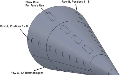
The model used in these tests is a 0.517-m-long 7° half-angle stainless-steel cone. Two different nose tips were tested; a sharp nose with a radius of less than 0.05 mm and a 0.5 mm radius blunt nose. There are two rows for instrumentation spaced 120° apart, with a third row installed 300° counter-clockwise from the first row, looking from the rear of the cone. Two of the rows have inserts which allow the installation of multiple types of sensors. The third row consists of 12 surface-mounted Medtherm Type-E coaxial thermocouples spaced 0.025 m apart, beginning at x = 0.222 m and ending at x = 0.497 m. The locations of the three rows are shown in Figure 1 and Table 1 lists the location of these sensors, where x is the axial distance from the sharp nose tip and φ is the cone azimuthal angle. More details about the cone, instrumentation and experiments are given in Reference 18. A photograph of the model installed in the Langley 20-Inch Mach 6 Tunnel is shown in Figure 2.
Table 1: Individual sensor locations for the two sensor insert rows.
Location x (m) φ (degrees) Sensor Type Location x (m) φ (degrees) Sensor Type
1A 0.208 0 Kulite 1B 0.208 120 PCB132 2A 0.246 0 Kulite 2B 0.246 120 PCB132 3A 0.284 0 Kulite 3B 0.284 120 PCB132 4A 0.322 0 Kulite 4B 0.322 120 PCB132 5A 0.360 0 Kulite 5B 0.360 120 PCB132 6A 0.398 0 Kulite 6B 0.398 120 PCB132 7A 0.452 0 Kulite 7B 0.452 120 PCB132 8A 0.490 0 Kulite 8B 0.490 120 PCB132
Figure 2: Photograph of model installed in the 20-Inch Mach 6 Tunnel.
The growth and breakdown of the second-mode wave instability was studied with PCB132 pressure sensors. The PCB132s were used to measure pressure fluctuations between 11 kHz and 1 MHz. The resonant frequency of the sensor is above 1 MHz and the sensor output is high-pass filtered with a 3-dB cutoff frequency at 11 kHz. Because of the good high frequency response of the sensors, the PCB132s are able to measure second-mode waves. They have been shown to have a flat response to 300 kHz.19 However, the sensors were designed as time-of-arrival
sensors and have not yet been accurately calibrated for instability measurements. The calibration uncertainty affects the amplitude of fluctuation measurements, but is unlikely to affect frequency measurement. In addition, there is some uncertainty about the spatial resolution of the sensors. The sensor diameter is 3.18 mm, but the sensing element is a 0.762 × 0.762-mm square. The surface of the sensor is coated with a conductive epoxy. It is uncertain how pressure is transmitted to the sensing element through this epoxy, so the active sensing area is unknown. It has been stated earlier that the sensing element size was 1 × 1.6 mm,18–22 but further communication with the sensor
manufacturer revealed that to be an error.
In order to compare the measured second-mode wave frequencies to computations, power spectral densities (PSD) were calculated from the PCB132 data. The PCB132 time traces were first normalized by the boundary-layer edge pressure, which was taken from the Taylor-Maccoll solution for a sharp cone. The power spectral densities were then calculated for record durations of 0.75 seconds using Welch’s method. A Blackman window of 1000 points was used, with 50 points of overlap between each window and the next. For each run, approximately 1970 FFTs were averaged. The frequency resolution for each PSD is about 2.4 kHz.
Pressure fluctuations with frequencies between 0 and 50 kHz were measured with Kulite Mic-062 sensors. The low-frequency pressure fluctuations measured by the Kulites peak near the end of transition.23–27 The location of this
peak can be compared to N factor computations from STABL, as well as transition location as measured by thermocouples.
Kulite pressure transducers use silicon diaphragms as the basic sensing mechanisms. Each diaphragm contains a fully active four-arm Wheatstone bridge. The Kulites have screens to protect the diaphragms from damage. The sensors used had A-type screens, which have a large central hole. This screen offers only a small amount of diaphragm protection, but gives a flatter frequency response. The sensitive area of the A-screen sensor is the hole size (0.81 mm2).
The Mic-062 Kulite microphone measures the pressure differential across a diaphragm up to ±7 kPa. The back side of the diaphragm has a pressure reference tube that is approximately 0.05 m long. This tube was bent 90 degrees to fit inside the model and left open to the plenum inside of the model. The plenum gives an approximately steady reference pressure, and high frequency components of this pressure are filtered by the long reference tube. The repeatability of the sensors is approximately 0.1% of the full scale (7 Pa).
C. Data Acquisition
The PCB132 sensors were all powered by a PCB 482A22 signal conditioner that provides constant-current excitation to the built-in sensor amplifier. The constant current can be varied from 4 to 20 mA; 4 mA was used for all measurements. The output from the signal conditioner was fed through a Krohn-Hite Model 3944 Filter with a 1 MHz lowpass anti-aliasing Bessel filter. This filter had four poles and offered 24 dB of attenuation per octave. The sampling frequency for the PCB132 sensors was 2.5 MHz. Data were acquired using a National Instruments PXI-1042 chassis with 14-bit PXI-6133 modules (10 MHz bandwidth) for data acquisition. This system was manually triggered once the model had reached the centerline of the test section, and data were acquired for 0.75 seconds. With the settings used here, this sample length fills the memory of the system.
A 10 V excitation was applied to the Kulites using an Endevco Model 136 DC Amplifier. The amplifier was also used to supply a gain of 100 for Kulite signal output. A Krohn-Hite Model 3384 Tunable Active Filter was used as a 200 kHz anti-aliasing low-pass Bessel filter for the Kulites. The filter had eight poles and provided 48 dB attenuation per octave. The Kulite data were acquired using the same system as described above and a sampling frequency of 1 MHz.
The thermocouple data were acquired using a 256-channel, 16 bit, 50 kHz or 100 kHz throughput rate, amplifier per channel, analog-to-digital (A/D) system manufactured by the NEFF Instrument Corporation. The system has programmable gains and filters per channel and an internal clock (System 620/series 600). The system is calibrated using an onboard calibration card. The thermocouple data were collected at a rate of 325 samples per second.
III.
Results
A. Summary of Data Obtained
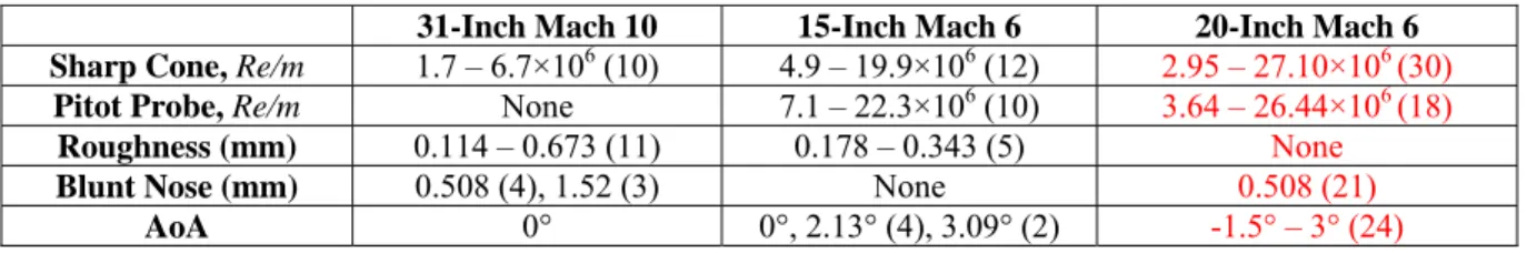
A large data set was obtained during these tests, and not all of it is presented in this paper. The data taken at NASA LaRC 15-Inch Mach 6 and 31-Inch Mach 10 Tunnels have been examined in detail and the results are presented in Reference 30. Table 3 summarizes the data obtained in each tunnel, with the current 20-Inch Mach 6 data shown in red. A total of 145 runs were made with the cone, with an additional 28 runs taking pitot acoustic noise measurements with a Kulite.
Table 2: Summary of data obtained in each of the LaRC facilities, numbers in parenthesis indicates the total number of runs completed for that case.
31-Inch Mach 10 15-Inch Mach 6 20-Inch Mach 6
Sharp Cone, Re/m 1.7 – 6.7×10⁶ (10) 4.9 – 19.9×10⁶ (12) 2.95 – 27.10×10⁶(30) Pitot Probe, Re/m None 7.1 – 22.3×10⁶ (10) 3.64 – 26.44×10⁶(18)
Roughness (mm) 0.114 – 0.673 (11) 0.178 – 0.343 (5) None
Blunt Nose (mm) 0.508 (4), 1.52 (3) None 0.508 (21)
B. Detection of Second-Mode Waves
Second-mode waves were successfully observed in all tunnels using the PCB132 sensors. This is the first time that instability waves have been measured in the Langley tunnels. Waves were detected in linear and non-linear stages of growth, as well as during breakdown. Though the 20-Inch Mach 6 test has been completed, not all the data has been fully analyzed. Once completed the results will be compared to the data from the 31-Inch Mach 10 and 15-Inch Mach 6 tests, for which comprehensive analyses have been completed.
Figure 3 shows spectra taken at two different unit Reynolds number conditions with the sharp nosetip installed and the cone at 0˚ AoA. Second mode waves appear as the large peaks in the spectra between about 200 kHz and 600 kHz. While computations are not yet available to confirm this identification, they are within the same frequency and magnitude range as previous measurements. Many examples of PCB measurements of second-mode waves with computations to confirm the identification are available in Reference 30.
The waves are observed to grow with downstream position, as expected. The frequency decreases with downstream position, which is due to the thickening of the boundary layer. The second-mode wavelength grows with the boundary-layer thickness, and with increasing wavelength the frequency decreases.
In these two cases, the waves eventually stop growing with downstream position, and the amplitude begins to decrease. This behavior indicates that the second-mode waves have saturated and begun to break down. As the waves break down, the prominent second-mode peak shrinks and disappears while the fluctuations at all frequencies begin to increase, eventually leading to a spectrum which shows no peak and high levels of fluctuations at all frequencies, as shown at x = 0.490 m in both plots. This type of spectrum indicates that the flow has become turbulent.
When the unit Reynolds number is increased, breakdown and transition move forward on the cone, as expected. For Re = 9.62x10⁶/m, waves are visible to x = 0.398 m, while for Re = 16.6x10⁶/m, they are only visible to x =
0.246 m. At the two locations where waves are visible for both conditions, the waves are much larger at the higher Reynolds number, as expected.
(b) 20-Inch Mach 6 Tunnel, Re/m = 16.55x10⁶
. (a) 20-Inch Mach 6 Tunnel, Re/m = 9.62x10⁶.
(a) Sharp Tip, x = 0.322 m. (b) Blunt Tip, x = 0.322 m. Figure 4: PCB measurements at representative unit Reynolds numbers with different nosetips.
Figure 4 shows spectra taken at x = 0.322 m across a range of unit Reynolds numbers with both a sharp and a blunt nosetip at 0˚ AoA. It should be noted that the position is really 0.322 m only for the sharp nosetip, since the blunt nosetip is 3.7 mm shorter. For the blunt nosetip, the same sensor is at x = 0.318 m. As observed in Figure 3, the waves at a given location typically grow with unit Reynolds number. In addition, the pattern of growth with unit Reynolds number appears very similar to the pattern of growth going downstream along the cone. The waves grow until they saturate, at which point they begin to break down, with the second-mode peak disappearing and the fluctuations at all frequencies increasing to high levels. One exception is that here the waves increase in frequency as they grow. This result is due to the boundary layer thinning as the unit Reynolds number is increased.
Comparing Figure 4(a) to Figure 4(b) reveals that, as expected, the second-mode waves are generally smaller with a blunt tip than with a sharp tip at a given position and unit Reynolds number. For example, at Re = 6.82x10⁶/m, the waves are hardly visible with the blunt nosetip, although they are fairly large with the sharp nosetip.
Also, transition is delayed, as expected. With a sharp nosetip, the waves have nearly disappeared for Re =
12.98x10⁶/m, and the second-mode peak has disappeared completely by Re = 16.6x10⁶/m. With a blunt nosetip, the
waves are clearly visible at Re = 16.6x10⁶/m, and disappear before Re = 21.8x10⁶/m. Additionally, the spectra at Re
= 11.9x10⁶/m for the sharp case and Re = 16.6x10⁶/m for the blunt case appear very similar.
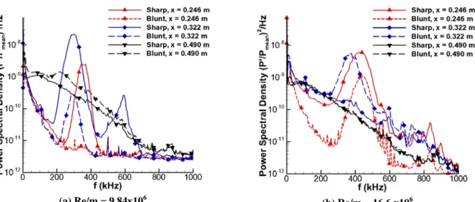
The spectra in the sharp and blunt cases can also be directly compared, allowing a more detailed
examination of the differences between the two cases. Figure 5(a) shows spectra taken from the same three sensors at Re = 9.84x10⁶/m with both a sharp nosetip and a blunt nosetip. At x = 0.246 m and x = 0.322 m, the reduction in
wave amplitude due to the blunt nosetip is obvious. At x = 0.246 m, the waves are not detected for the blunt case, while they are significant for the sharp case. The waves appear at x = 0.322 m for the blunt case, but are small. In the sharp case at the same position, the waves are large and nonlinear, as indicated by the higher harmonic visible near 600 kHz. At x = 0.490 m, by contrast, the spectra are very similar between the two cases. While the waves have completely disappeared in the sharp case, it appears there may still be a small peak visible near 200 kHz in the blunt case. For most of the frequency range, the fluctuations in the blunt case are higher than in the sharp case, but follow nearly the same curve.
Figure 5(b) shows the same comparison, but for Re = 16.6x10⁶/m. Once again, the waves are much smaller
for the blunt case than for the sharp case at x = 0.246 m. At x = 0.322 m, the waves are actually larger for the blunt case than for the sharp case. This is because the waves have broken down almost completely in the sharp case, while the waves in the blunt case are only in the late nonlinear stages of growth. At x = 0.490 m, the spectra indicate turbulence in both cases and have become almost indistinguishable. This is expected, since a turbulent spectrum should not depend on the path to transition.
(a) Re/m = 9.84x10⁶ (b) Re/m = 16.6 x10⁶
Figure 5: Spectra comparisons between sharp and blunt nosetips.
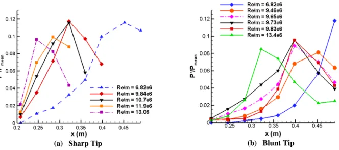
The RMS amplitudes of the second-mode waves were also computed. Since the calibration of the PCB-132 sensors is uncertain for instability measurements, the actual values reported should be considered as reasonable estimates. Figure 6 shows the second-mode amplitudes for every sensor over a range of unit Reynolds numbers. In general, the amplitudes increase both with increasing unit Reynolds number and with increasing position. As before, eventually the waves saturate and begin to break down, and the amplitudes decrease. Figure 6(a) shows that for the sharp case, the maximum RMS amplitude is typically close to 11% of the mean. The maximum amplitude tends to decrease as the unit Reynolds number is increased and saturation moves forward.This decrease may be a real effect, though it may also be due to the spatial resolution of the sensors. As saturation moves forward, the wavelength at the point of saturation decreases, increasing the effect of spatial averaging on the measurement and decreasing the measured RMS value. In addition, the peak may be falling between two sensors, since the breakdown process appears to take place within a short distance. Measurements with a denser sensor spacing are necessary to determine how well the peak amplitude is being resolved.
A saturation amplitude of 11% agrees well with the observed saturation amplitude of 12% in the
Boeing/AFOSR Mach 6 Quiet Tunnel (BAM6QT) at Purdue when run noisy.7 The maximum amplitude observed in
the 15-Inch Mach 6 Hi-Temperature tunnel was only 8%, but the peaks may not have been properly resolved in that tunnel due to the wide sensor spacing used in those tests (PCB sensors were located only at positions x=0.208, 0.360 and 0.490m). Saturation amplitudes have previously been observed to vary from as low as 5% at Mach 5 to as much as 30% at Mach 10.16 The main determinant of the saturation amplitude is unknown.
Figure 6(b) shows RMS amplitudes of the second-mode waves with the blunt nosetip installed. Not as many runs were performed with the blunt nosetip, so the Reynolds number sweep is not as dense or evenly spaced as for the sharp case. The amplitude curves for the blunt case are very similar to those for the sharp case, except that the amplitudes are generally smaller for any given position and unit Reynolds number. In addition, the maximum amplitudes for the blunt case are typically around 9%, while those for the sharp case were typically close to 11%. One value near 12% was observed for the blunt case. It is not clear if the difference in saturation amplitudes between the two nose radii is a real effect, or if the saturation peaks were just not as well-resolved for the blunt case. A denser Reynolds number sweep and/or sensor spacing for the blunt case is necessary to better resolve the saturation peak.
(a) Sharp Tip (b) Blunt Tip Figure 6: Second-mode amplitudes computed from PCB spectra.
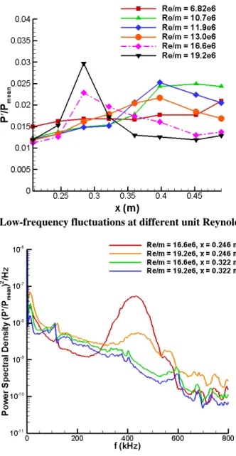
C. Low-Frequency Fluctuations
The Kulite sensors provide another way of looking at transition. The peak in the pressure fluctuations occurs near the end of transition, and so would be expected to occur downstream of the position where the second-mode waves break down. Here, the fluctuations are normalized by edge pressure, which collapses the laminar fluctuations fairly well for this case. Figure 7 shows the normalized fluctuations for a range of Reynolds numbers.
Transition is indicated by a peak in the level of fluctuations. Here, the peaks are not always easily identified, which might suggest that the peaks are typically falling in between two sensors. However, despite this difficulty, the generally expected trends can be identified. At Re = 6.82x10⁶/m, no peak is present. This result agrees well with the
observation that second-mode waves are still present at the last sensor at this condition. At Re = 10.7x10⁶/m, the
peak is not well-resolved, though there is a sharp rise in the level of fluctuations at x = 0.398 m. The maximum fluctuation level is observed at x = 0.452 m, with similar levels of fluctuations observed at x = 0.490 m. The transitional peak appears to have occurred somewhere in this region, though the exact location is unclear. At this condition, the second-mode waves have broken down by x = 0.360 m (Figure 6(a)), which agrees with the presence of a transitional peak somewhere farther downstream.
The transitional peak is more clearly defined for Re = 11.9x10⁶/m, occurring at x = 0.398 m. For Re =
13.0x10⁶/m the transitional peak decreases in magnitude but does not appear to move. This suggests that the peak
has moved forward of x = 0.398 m. For these two cases, the second-mode waves also disappear after the same sensor location, x = 0.322 m, as shown in Figure 6(a). However, the amplitude is much smaller for the higher unit Reynolds number, suggesting that breakdown is more complete and that transition has moved forward.
The transitional peak then moves much farther forward on the cone, to x = 0.284 m, for the highest two Reynolds number conditions. The peak is particularly sharp for Re = 19.2x10⁶/m, suggesting that the sensor was
very close to the actual peak in low-frequency fluctuations. In both of these cases, the second-mode waves have disappeared by x = 0.322 m, but are visible at x = 0.246 m as illustrated in the PCB data shown in Figure 8. However, for Re = 19.2x10⁶/m, the waves have nearly disappeared at x = 0.246 m, indicating that breakdown and
Figure 7: Low-frequency fluctuations at different unit Reynolds numbers.
Figure 8: Spectra comparisons of the PCB data at high Reynolds numbers.
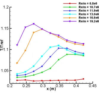
D. Preliminary Thermocouple Data
The thermocouple data can be used as a reference for locating transition on the cone. Due to time constraints, the Stanton number was not computed. However, the ratio of the thermocouple temperature to the run reference temperature was computed and plotted versus axial location in Figure 9. Laminar flow is evidenced by low, fairly constant temperature ratios, transitional flow by temperature ratios that increase with x, and turbulent flow by the higher temperature ratios that decrease with x.
The Kulites and thermocouples both show very similar trends for all unit Reynolds numbers. The sensor spacing of the thermocouples is denser than that of the Kulites, so the location of transition may be easier to determine from the thermocouple data. Both the Kulites and thermocouples indicated the flow is laminar along the entire length of the cone for the 6.8x10⁶/m Reynolds number case. A forward movement of transition is also
indicated in both sets of data, as can be seen in Figures 6 and 8. At the highest Reynolds numbers shown here, the peaks of the Kulite data are seen at x = 0.284m which is very close to the peaks seen in the thermocouple data at x = 0.272m for Re = 19.2x10⁶/m and x = 0.297 for Re = 16.6x10⁶/m.
Though more analysis needs to be performed on the thermocouple data to draw any real conclusions, the temperature ratio shown here is a good indication of the transition location at any given Reynolds number. Better comparisons can be made once the Stanton number has been calculated.
Figure 9: Temperature ratios along the cone at various unit Reynolds numbers.
E. Preliminary Tunnel-to-Tunnel Comparison
As stated previously, the present measurements were made as part of an effort to show that boundary-layer instabilities can be measured in large conventional hypersonic tunnels, and to better determine the effect of tunnel noise on transition. The cone model was previously tested, under similar conditions, in both the Langley 15-Inch Mach 6 tunnel16 and the Boeing/AFOSR Mach 6 Quiet Tunnel at Purdue University run under both noisy and quiet
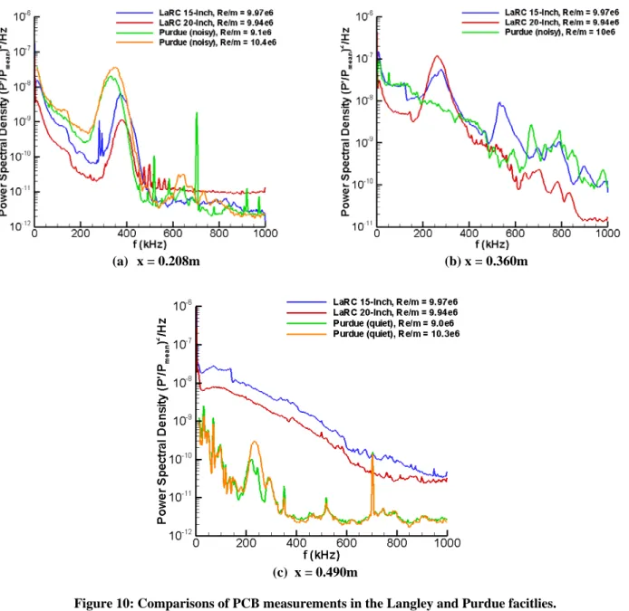
conditions8. Figure 10 shows PCB data from the same axial location on the cone in each of these tunnels for Re/m ≈
10x106. Figure 10(a) shows data at x = 0.208m for both of Langley’s facilities as well as the Purdue tunnel run
noisy. The waves are larger in the 15-Inch Tunnel than the 20-Inch Tunnel, and the waves in the Purdue tunnel are much larger than in both of the Langley tunnels. The waves in the Purdue tunnel also show a possible harmonic developing at 650kHz, which is not present in either of the Langley tunnels at this condition. It should also be noted the Purdue spectra show waves of a lower frequency than those from the Langley tunnels, though the reason for this difference is not clear.
Figure 10(b) shows similar comparisons for the PCBs located at x = 0.360m. At this location, the spectrum in the Purdue case indicates that the second-nose waves have broken down completely and disappeared. For both the Langley tunnels; however, waves are still clearly visible near 275 kHz. This would suggest higher freestream noise levels in the Purdue tunnel when run noisy than in the Langley tunnels. Higher freestream noise levels would be expected to cause higher initial wave amplitudes, leading to larger waves at a given Reynolds number and causing breakdown and transition to occur at lower Reynolds numbers, as observed here.
In Figure 10(c), spectra from the Langley tests are compared to the Purdue tunnel when run under quiet conditions at x = 0.490m. While the flow appears to be turbulent at this location in the Langley tunnels and under noisy flow in the Purdue tunnel, under quiet conditions the boundary layer is laminar with very small second-mode waves.
This figure helps to illustrate the effect of tunnel noise on transition. Once a full tunnel noise characterization study has been completed in the Langley facilities, it is hoped that a method for extrapolating transition location between ground test facilities and from ground test to flight can be established.
(a) x = 0.208m (b) x = 0.360m
(c) x = 0.490m
Figure 10: Comparisons of PCB measurements in the Langley and Purdue facitlies.
IV. Conclusions
Second-mode waves were successfully measured for the first time in the Langley 20-Inch Mach 6 tunnel. The growth, saturation, and breakdown of the waves were observed both with a sharp nosetip and a blunt nosetip. The saturation amplitude was observed to be about 11% of the mean pressure, consistent with previous observations in other hypersonic tunnels. In particular, this saturation amplitude was very similar to that observed by Casper et al. in the BAM6QT at Purdue, which was 12%. The maximum amplitudes observed with a blunt nosetip installed were slightly smaller than those with the sharp nosetip, about 9%. However, it is not clear if this is a real difference, or if the peaks were just not resolved well enough to capture the highest amplitudes. The general patterns of growth and breakdown were observed to be very similar in both the sharp and blunt cases, though in the blunt case the waves were smaller at a given condition and transition was delayed. Turbulent spectra in the two cases were observed to be essentially identical, as expected.
Measurements of low-frequency fluctuations were also performed, providing a method of measuring the location of the end of transition. The peak in low-frequency fluctuations typically followed the expected trends, although the sensor spacing was wide enough that it was not well-resolved for every case. Thermocouple measurements were also obtained, providing a another indication of the transition location. These results were consistent with the measurements of the other two sensor types.
PCB measurements from the Langley Mach 6 facilities were compared to similar data from the
Boeing/AFOSR Mach 6 Quiet Tunnel at Purdue. Wave breakdown appeared to occur earlier in the Purdue tunnel under noisy condition than in the Langley tunnels, but under quiet conditions only very small waves were observed. These comparisons help to illustrate the effect of tunnel noise on instability growth and transition.
In the future, the second-mode wave and transition measurements should be compared to pitot probe measurements of the freestream acoustic noise. Some measurements of this noise have been performed, but have yet to be compared to the measurements on the cone. In addition, the PCB sensors should be calibrated so that accurate second-mode amplitudes can be obtained. Computations are also necessary so that the results can be compared to theoretical predictions of the growth of the waves.
V. Acknowledgements
This work could not have been completed without the generosity of Sandia National Laboratories and Katya Casper. The model used to perform these tests was designed and built by Sandia for Ms. Casper’s Ph.D research and loaned to Langley during the duration of these tests.
The authors would also like to acknowledge the support of the Exploration Technology Development and Demonstration (ETDD) Program, managed at NASA-Glenn Research Center. The work documented herein was performed as part of ETDD’s Entry, Descent, and Landing (EDL) Technology Development Project, which is managed at NASA-Langley Research Center and supported by NASA-Ames Research Center, NASA-Johnson Space Center, and the Jet Propulsion Laboratory.
References
1Mack, L. M., “Boundary-Layer Linear Stability Theory,” Special Course on Stability and Transition of
Laminar Flow, AGARD-R-709, chap. 3, June 1984, pp. 3–1:3–81.
2Stetson, K., Kimmel, R., Thompson, E., Donaldson, J., and Siler, L., “A Comparison of Planar and Conical
Boundary Layer Stability at a Mach Number of 8,” AIAA Paper 91-1639, June 1991.
3Stetson, K. F. and Kimmel, R. L., “Example of Second-Mode Instability Dominance at a Mach Number of
5.2,” AIAA Journal , Vol. 30, No. 12, December 1992, pp. 2974–2976.
4Schneider, S. P., “Hypersonic Laminar-Turbulent Transition on Circular Cones and Scramjet Forebodies,”
Progress in Aerospace Sciences, Vol. 40, 2004, pp. 1–50.
5Rufer, S. J., and Schneider, S. P., “Hot-Wire Measurements of Instability Waves on Cones at Mach 6,” AIAA
Paper 2006-3054, June 2006.
6Fujii, K., “Experiment of Two Dimensional Roughness Effect on Hypersonic Boundary-Layer Transition,”
Journal of Spacecraft and Rockets, Vol. 43, No. 4, July-August 2006, pp. 731–738.
7Estorf, M., Radespiel, R., Schneider, S. P., Johnson, H., and Hein, S., “Surface-Pressure Measurements of
Second- Mode Instability in Quiet Hypersonic Flow,” AIAA Paper 2008-1153, January 2008.
8Casper, K. M., Beresh, S. J., Henfling, J. F., Spillers, R. W., Pruett, B., and Schneider, S. P., “Hypersonic
Wind-Tunnel Measurements of Boundary-Layer Pressure Fluctuations,” AIAA Paper 2009-4054, June 2009, revised November 2009.
9Tanno, H., Komuro, T., Sato, K., Itoh, K., Takahashi, M., and Fujii, K., “Measurement of Hypersonic
Boundary Layer Transition on Cone Models in the Free-Piston Shock Tunnel HIEST,” AIAA Paper 2009-0781, January 2009.
10Beckwith, I. E. and Miller III, C. G., “Aerothermodynamics and Transition in High-Speed Wind Tunnels at
NASA Langley,” Annual Review of Fluid Mechanics, Vol. 22, 1991, pp. 419–439.
11Schneider, S. P., “Flight Data for Boundary-Layer Transition at Hypersonic and Supersonic Speeds,”
Journal of Spacecraft and Rockets, Vol. 36, No. 1, 1999, pp. 8–20.
12Chen, F.-J., Malik, M., and Beckwith, I., “Boundary-Layer Transition on a Cone and Flat Plate at Mach 3.5,”
13Ward, C., Wheaton, B. M., Chou, A., Gilbert, P. L., Steen, L. E., and Schneider, S. P., “Hypersonic
Boundary-Layer Transition Experiments in a Mach-6 Quiet Tunnel,” AIAA Paper 2010-4721, June 2010.
14Alba, C., Johnson, H., Bartkowicz, M., Candler, G., and Berger, K., “Boundary Layer Stability Calculations
for the HIFiRE-1 Transition Experiment,” Journal of Spacecraft and Rockets, Vol. 45, No. 6, January 2008, pp. 1125–1133.
15Pate, S. R., “Measurements and Correlations of Transition Reynolds Numbers on Sharp Slender Cones at
High Speeds,” AIAA Journal, Vol. 9, No. 6, 1971, pp. 1082–1090.
16Berridge, D. C., Casper, K. M., Rufer, S. J., Alba, C. R., Lewis, D.R., Beresh, S. J., and Schneider, S. P.,
“Measurements and Computations of Second-Mode Instability Waves in Three Hypersonic Wind Tunnels,” AIAA Paper 2010-5002, June 2010.
17Micol, J. R., “Langley Aerothermodynamics Facilities Complex: Enhancements and Testing Capabilities,”
AIAA Paper 1998-0147, January 1998.
18Casper, K. M., Hypersonic Wind-Tunnel Measurements of Boundary-Layer Pressure Fluctuations, Master’s
thesis, Purdue University School of Aeronautics and Astronautics, August 2009.
19Beresh, S., Henfling, J., Spillers, R., and Pruett, B., “Measurement of Fluctuating Wall Pressures Beneath a
Supersonic Turbulent Boundary Layer,” AIAA Paper 2010-305, January 2010.
20Wheaton, B. M., Juliano, T. J., Berridge, D. C., Chou, A., Gilbert, P. L., Casper, K. M., Steen, L. E.,
Schneider, S. P., and Johnson, H. B., “Instability and Transition Measurements in the Mach-6 Quiet Tunnel,” AIAA Paper 2009-3559, June 2009.
21Alba, C., Casper, K., Beresh, S., and Schneider, S., “Comparison of Experimentally Measured and Computed
Second-Mode Disturbances in Hypersonic Boundary-Layers,” AIAA Paper 2010-897, January 2010.
22Berridge, D., Chou, A., Ward, C., Steen, L., Gilbert, P., Juliano, T., Schneider, S., and Gronvall, J.,
“Hypersonic Boundary-Layer Transition Experiments in a Mach-6 Quiet Tunnel,” AIAA Paper 2010-1061, January 2010.
23Pate, S. R. and Brown, M. D., “Acoustic Measurements in Supersonic Transitional Boundary Layers,” Tech.
Rep. AEDCTR-69-182, Arnold Engineering Development Center, October 1969.
24Johnson, R. I., Macourek, M. N., and Saunders, H., “Boundary Layer Acoustic Measurements in Transitional
and Turbulent Flow at M∞ = 4.0,” AIAA Paper 69-344, April 1969.
25Cassanto, J. M. and Rogers, D. A., “An Experiment to Determine Nose Tip Transition with Fluctuating
Pressure Measurements,” AIAA Journal, Vol. 13, No. 10, 1975, pp. 1257–1258.
26Martellucci, A., Chaump, L., Rogers, D., and Smith, D., “Experimental Determination of the Aeroacoustic
Environment about a Slender Cone,” AIAA Journal, Vol. 11, No. 5, 1973, pp. 635–642.
27Pate, S. R., “Dominance of Radiated Aerodynamic Noise on Boundary-Layer Transition in
Supersonic/Hypersonic Wind Tunnels,” Tech. Rep. AEDC-TR-77-107, Arnold Engineering Development Center, March 1978.
28Wright, M. J., Candler, G. V., and Bose, D., “A Data-Parallel Line-Relaxation Method for the Navier-Stokes
Equations,” AIAA Paper 97-2046CP, June 1997.
29Johnson, H. B. and Candler, G. V., “Hypersonic Boundary Layer Stability Analysis Using PSE-Chem,” AIAA
Paper 2005-5023, June 2005.
30Berridge, D., Measurements of Second-Mode Waves in Hypersonic Boundary Layers with a High-Frequency