Multi-fluid Dynamics for Supersonic Jet-and-Crossflows and Liquid Plug Rupture by
Ezeldin A. Hassan
A dissertation submitted in partial fulfillment of the requirements for the degree of
Doctor of Philosophy (Aerospace Engineering) in the University of Michigan
2012
Doctoral Committee:
Professor Wei Shyy, Co-Chair Professor Ken Powell, Co-Chair Professor James F. Driscoll Professor Hong G. Im
© Ezeldin A. Hassan 2012
ii
iii Acknowledgment
I would like to thank my advisor Prof. Wei Shyy for his unwavering support and advice both academically and personally. He has always made his students a priority and set an example that is very hard to follow. I consider myself lucky to have received such valuable well-rounded mentoring that served to shape the essence of the person I am today. I would also like to thank my co-chair Prof Ken Powell and my committee Prof. James Driscoll, Prof. Hong Im and Dr. Doug Davis for their help with my dissertation.
I would like to thank Dr Doug Davis also for being my mentor at AFRL propulsion directorate and for his insight and inspirational research support. I would like to thank Dr. John Boles at AFRL for continuous help and research collaboration regarding supersonic jet and crossflow interaction. I would like to thank all the research scientists who have helped me through my internships at AFRL; Dr. Mark Hagenmaier, Dr. Daniel Risha, Dr. Dean Eklund, and others. I would like to thank Dr. Tom Jackson and the propulsion directorate as a whole for accepting to serve as my sponsoring facility and showing interest in my research and future collaboration with AFRL. I would like to also thank HPCMO-DSRC for computer time.
I would like to thank my research collaborators specifically Dr. Hikaru Aono for his assistance, sincere advice, and collaboration with supersonic jet and crossflow interaction research and other issues, Dr. Emre Sozer for invaluable discussion and insight regarding CFD code development and numerical methods, and Dr. Jaeheon Sim for assisting in multiphase flow research. I would like to thank Dr Eray Uzgoren, Dr. James Grotberg and Dr. Hideki Fujioka for their collaboration on the plug flow problem.
I would like to thank Dr. Ed Luke, Dr. Jeff Wright and Dr. ST Thakur for their support with Loci-Chem. They have helped me with many questions regarding code structure and development.
I would like to thank my group members, office mates in FXB2211, and students in the other side of the FXB for the continuous friendship and support. Especially, I
iv
would like to thank Dr. Chang-kwon Kang for his help in dissertation formatting issues, Dr. Amit Gupta, Dr. Pat Trizila, and Dr. Chien-Chou Tseng, Dr. Young-Chang Cho, Wenbo Du, Chih-Kuang Kuan, and Dr. Hicham Alkandry.
I would like to thank the SMART program for funding and supporting my research and for linking me with AFRL. I would like to thank SMART staff specifically; Alexis Becker and Danielle Rinderknecht for their help and support with the lengthy SMART paperwork. I would like to thank Brian Padilla my security officer for helping me with numerous security issues.
I would like to thank the staff in the aerospace department not only for their work, but also for creating a friendly environment in the FXB building, in particular Cynthia Enoch, Dave McLean, Denise Phelps, Michelle Shepherd, Sue Smith, and Lisa Szuma.
Finally, I would like to thank my family and friends. I would like to thank my wife, my parents, and my brothers and sister for their endless support and love. Furthermore, I would like to thank all those that I have not named.
v Table of Contents
Dedication ... ii
Acknowledgment ... iii
List of Figures ... viii
List of Tables ... xiii
List of Symbols ... xiv
List of Abbreviation ... xviii
Abstract ... xix
Chapter 1. Background and Motivation ... 1
1.1 Introduction and Scope ... 3
1.2 Motivation ... 5
1.3 The SCRAMJET Engine ... 7
1.3.1 SCRAMJET Engine Components ... 8
1.3.2 SCRAMJET Advantages and Challenges ... 10
1.4 Mixing and Structure of Supersonic Jet and Crossflow ... 12
1.5 Experimental Studies of Supersonic Jet and Crossflow ... 15
1.6 Scaling Efforts for Supersonic Jet and Crossflow ... 19
1.7 Computational Approaches for Jet and Crossflow ... 20
1.8 Mixing of Liquid Jets ... 29
1.9 Plug Flow and Rupture Problem ... 30
1.10 Multiphase Flow Methods ... 35
1.11 Objectives and Proposed Models ... 36
1.11.1 Jet and Crossflow Interaction ... 36
1.11.2 Plug Propagation and Rupture ... 39
Chapter 2. Governing Equations and Numerical Methods ... 40
2.1 Governing Equations ... 40
2.1.1 Instantanous Balance Equations ... 40
2.1.2 Equation of State ... 41
2.1.3 Averaged and Filtered Navier-Stokes Equations ... 42
2.1.4 Turbulence Closure ... 44
2.2 Turbulence Modeling ... 45
vi
2.2.2 LES: Smagorinsky Lilly Model ... 51
2.2.3 Hybrid RANS/LES: NC State Model ... 52
2.2.4 Detached Eddy Simulation (DES) ... 54
2.2.5 Filter Based Approach ... 56
2.3 Current Modeling Approach ... 58
2.3.1 Multi-scale Turbulent Treatment ... 59
2.3.2 Adaptive Turbulent Schmidt Number Extension ... 67
2.4 Numerical Methodology ... 70
2.4.1 Base CFD Code ... 70
2.4.2 Implementation of Current Model ... 72
Chapter 3. Multi-scale Turbulence Modeling for Supersonic Jet and Crossflow ... 77
3.1 Experimental Setup ... 77
3.2 Computational Parameters ... 79
3.3 Nozzle Simulation ... 82
3.4 Sonic Injection Cases ... 83
3.4.1 Baseline Case: 90o, q=0.5 [Cases 1-8] ... 85
3.4.2 Non-Baseline [Cases 9-14] ... 104
3.5 Assessment of Multi-scale Model Performance ... 112
3.6 Summary ... 115
Chapter 4. Adaptive Turbulent Schmidt Number in Turbulence Modeling ... 117
4.1 Implications of The Adaptive Approach ... 117
4.2 Baseline Case: 90o,q=0.5 [Cases 15-19] ... 120
4.2.1 Adaptive multi-scale and comparison to constant multi-scale and RANS results ... 121
4.2.2 Effect of Numerical Viscosity on Turbulent Diffusivity ... 124
4.2.3 Adaptive Turbulent Schmidt Number Effect on Solution and Mixing ... 129
4.3 Inclined Case : 30o, q=0.5 ... 132
4.4 Summary ... 138
Chapter 5. Propagation and Rupture of Incompressible Liquid Plug in a Tube ... 139
5.1 Model Description ... 140
5.2 Computational Procedure ... 141
5.2.1 Surface Tension Treatment ... 143
5.2.2 Interface Reconstruction Scheme ... 144
vii
5.2.4 Adaptive Time Stepping ... 149
5.3 Results and Discussion ... 150
5.3.1 Pre-Rupture Dynamics ... 150
5.3.2 Rupture Dynamics ... 155
5.3.3 Effects of Pressure Drop and Laplace number... 163
5.4 Summary ... 167
Chapter 6. Concluding Remarks ... 170
6.1 Summary and Conclusions ... 170
6.2 Future Work ... 176
6.2.1 Jet and Crossflow Interaction ... 176
6.2.2 Plug Propagation and Rupture ... 178
viii List of Figures
Figure 1-1 Specific Impulses for Several Engine Cycles[56] ... 8 Figure 1-2 Diagram of a SCRAMJET engine, highlighting major components[57] ... 9 Figure 1-3 Model of transverse underexpanded jet in a supersonic crossflow (a)Full 3D
schematic from Portz and Segal[60] (b) cross section schematic near injector from Gruber et al [8] ... 13 Figure 1-4 Indented Barrel shock with recirculation regions in normal sonic air injection
into Mach 4 crossflow from Viti et al [17] ... 14 Figure 1-5 Temporally-resolved shadowgraphs of Mach 1.6, q=1.7 Air/Air jet and
crossflow by VanLerberghe et al[50] ... 17 Figure 1-6 Penetration heights compared to the experiment for 3 turbulent models from
Tam et al[19] ... 23 Figure 1-7 Experimental, RANS and Hybrid RANS/LES concentration comparison from Boles et al[27] ... 26 Figure 1-8 Live-dead staining of human pulmonary epithelial cells after 10(a),50(b), and
100(c) plug propagation events from Tavana et al [99] ... 31 Figure 1-9 Interface representation by marker points (a) line segments in 2D (b)
triangular elements in 3D (c) indicator function used to smear properties across the interface with values varying from 0 to 1[48] ... 35 Figure 2-1 NC State blending function and velocity boundary-layer in wall coordinates 53 Figure 2-2 Filter functions for FBM, multi-scale models and proposed filter ... 63 Figure 2-3 Cell-neighbor notation in an unstructured grid ... 71 Figure 2-4 Flow chart of the solution procedure using the multi-scale model ... 74 Figure 2-5 Flow chart of the solution procedure using multi-scale model with the
adaptive approach ... 76 Figure 3-1 Injector shape and placement for (a) normal injection and (b) inclined
injection... 78 Figure 3-2 Pressure probe data at x/D=5, y/D=0.25 and z/D=0.25 for 30 degree injection.
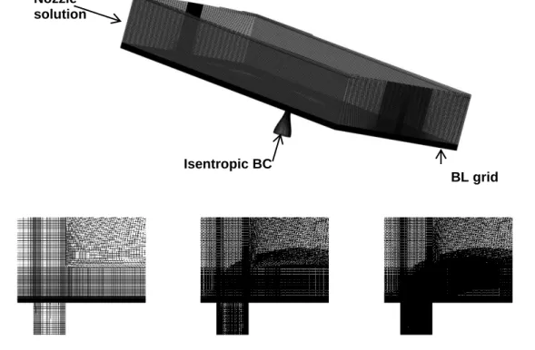
Flow is considered statistically converged and iterations are used to collect average ... 81 Figure 3-3 Computational domain and boundary conditions for jet and crossflow
ix
Figure 3-4 Nozzle simulation(right): outflow boundary-layer axial velocity and
turbulence kinetic energy, grid distribution for outflow boundary(left) ... 83 Figure 3-5 Grid distribution and boundary conditions for normal injection (top). Center
plane cut: coarse, intermediate and fine grids in order ... 85 Figure 3-6 Pressure iso-surface (bow shock), midline average ethylene mole fraction
(midline plane), and selected streamlines showing spilled vortex (baseline case, intermediate grid) ... 86 Figure 3-7 Snapshot of Mach number on the midline plane showing the barrel shock.
White line outlines the jet profile at ethylene mole fraction of 0.05 (baseline, intermediate grid) ... 87 Figure 3-8 Average ethylene mole fraction results for RANS with different turbulent
Schmidt numbers comparison with experiment. (baseline case) ... 89 Figure 3-9 Sample NOPLIF images for the baseline case for x/D=5 (top) and x/D=25
(bottom)... 90 Figure 3-10 mean and variance of fuel concentration for RANS, multi-scale and
experimental NO PLIF images(baseline case) ... 90 Figure 3-11 Instantaneous snapshots of ethylene mole fraction contours for coarse,
intermediate, and fine grids(baseline case) ... 91 Figure 3-12 Instantaneous snapshots of eddy viscosity contours for coarse, intermediate,
and fine grids(baseline case) ... 92 Figure 3-13 Average ethylene mole fraction results for grid refinement study(baseline
case) ... 94 Figure 3-14 Centers for fuel penetration((a) height, (b)widths) for experiment, RANS,
and multi-scale models (baseline case) ... 95 Figure 3-15 Pressure on the center plane. Comparison between RANS and multi-scale
computation(baseline case) ... 96 Figure 3-16 Axial velocity on center plane. Comparison between RANS and
multi-scale(baseline case) ... 97 Figure 3-17 Contours of P/P∞ on bottom wall. RANS and multi-scale predictions
compared to PSP (baseline case) ... 98 Figure 3-18 P/P∞ on the surface at z/D=0(baseline case) ... 98 Figure 3-19 Turbulence kinetic energy (KRes, bottom) and ratio of unresolved turbulence
kinetic energy to total turbulence kinetic energy (KRatio, top) (baseline case) .... 101 Figure 3-20 Instantaneous vorticity snapshots on the center plane for multi-scale
(intermediate grid on top and coarse grid on the bottom) and MILES (coarse) approaches. Maximum and minimum limited to 100, -100 ... 102 Figure 3-21 Mass and momentum eddy viscosities based on resolved field at the center
plane (baseline case) ... 103 Figure 3-22 Mass and momentum eddy viscosities as well as effective turbulent Schmidt
x
number based on resolved field for x/D= 5 intermediate grid (baseline case).... 105 Figure 3-23 Baseline ethylene mole fractions comparison, intermediate grid (baseline
case) ... 106 Figure 3-24 Grid distribution and boundary conditions for inclined injection (top). Center plane cut: RANS and multi-scale grids in order(bottom) ... 107 Figure 3-25 Average ethylene mole fractions comparison, RANS and multi-scale (90o,
q=1.5) ... 108 Figure 3-26 Average ethylene mole fractions comparison, RANS and multi-scale (30o,
q=1.0) ... 109 Figure 3-27 Average mole fraction predictions for RANS and multi-scale compared to
experimental Raman scattering at 3 different axial locations. (30o,q=0.5) ... 110 Figure 3-28 Centers for fuel penetration((a) height, (b)widths) for experiment, RANS,
and multi-scale models (30o,q=0.5) ... 111 Figure 3-29 Vorticity in the y plane ( out of the paper) for different injection
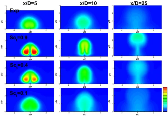
configurations on the center plane Maximum and minimum limited to 100, -100 ... 113 Figure 4-1 Adaptive turbulent Schmidt number contours for grid 1(top) and 2 (bottom) at different locations (baseline case) ... 122 Figure 4-2 Fuel mole fraction contours at = 5 for experimental and different
numerical approaches. In multi-scale simulations grid 1 results are on top and grid 2 on the bottom ... 123 Figure 4-3 Fuel mole fraction contours at = 25 for experimental and different
numerical approaches. In multi-scale simulations grid 1 results are on top and grid 2 on the bottom ... 124 Figure 4-4 (repeated from 3-16) Instantaneous vorticity snapshots on the center plane
for multi-scale (grid 2 on top and grid 1 on the bottom) and MILES (grid1) approaches. Maximum and minimum limited to 100, -100 ... 126 Figure 4-5 Instantaneous fuel mole fraction snapshots on the center plane for multi-scale
(grid 2 on top and grid 1 on the bottom) and MILES ( grid1) approaches (baseline case) ... 127 Figure 4-6 Fuel mole fraction predictions for the multi-scale adaptive approach with
numerical viscosity correction. Experimental measurements on the top, grid 1 in the middle and grid 2 on the bottom ... 128 Figure 4-7 Average bow shock pressure iso-surface and fuel streamlines for case 6.
Average fuel mole fractions iso-surfaces for cases 5, 18, and 6. ... 130 Figure 4-8 Average fuel mole fractions at center plane for cases 5, 18, and 6.. ... 131 Figure 4-9 Center plane pressure contours for cases 6 and 18. Injector is located at =
0... 131 Figure 4-10 Center plane axial velocity contours for cases 6 and 18. Injector is located at
xi
= 0 ... 132 Figure 4-11 Mean intensity of PLIF images (2 separate images taken) compared to fuel
mole fraction contours in grey scale of RANS ,multi-scale, and adaptive
models(30o,q=0.5). ... 133 Figure 4-12 Variance of intensity of PLIF images(2 separate images taken) compared to
fuel mole fraction variance contours in grey scale of RANS , multi-scale, and adaptive models(30o,q=0.5). ... 134 Figure 4-13 Fuel mole fraction predictions for multi-scale with/without the adaptive
approach compared to experimental Raman scattering at 3 different axial
locations(30o,q=0.5). ... 136 Figure 4-14 Centers for fuel penetration((a) height, (b)widths) for experiment, RANS,
and multi-scale with and without the adaptive approach (30o,q=0.5)... 137 Figure 4-15 Adaptive turbulent Schmidt number contours for at different
locations(30o,q=0.5). ... 137 Figure 5-1 Computational setup and the boundary conditions, x axis attached to plug
center before rupture and to the wall afterwards. Plug moves to the right ... 140 Figure 5-2 Identification of necking, a possible cause for topological change ... 145 Figure 5-3 Summary of the reconstruction algorithm in 2D and 3D ... 146 Figure 5-4 Reconstruction scheme. (a) Two interfaces come close so that the distance for red markers are less than critical length, (b) forming a single interface by updating the connectivity information ... 147 Figure 5-5 Geometry based grid refinement around the interface at various resolutions149 Figure 5-6 Plug length variation in time for various initial precursor film thickness
values. Solid lines represent present study while dots represent study of [53]. (b) shows a more confined time domain to show details ... 151 Figure 5-7 Course of plug speed, defined as the capillary number, in time for various
initial precursor film thickness values. Solid lines represent present study while dots represent study of [53]. (b) shows progressively zoomed in views of the plot in (a) ... 152 Figure 5-8 (a)Pressure and shear stress variation at the airway walls before plug rupture
when Lp = 0.3, P = 1, and = 1000. Solid lines represent present study while dots represent study of [53] (b) Pressure contours and velocity vectors near the wall corresponding to ... 156 Figure 5-9 Snapshots of pressure contours before and after rupture. h2 = 0.06, P = 1, and
= 1000. ... 157 Figure 5-10 Pressure contours, velocity vectors and wall pressure and wall shear stress
prior to rupture for h2=0.06. View is zoomed at the location of minimum film thickness ... 158 Figure 5-11 Pressure contours, velocity vectors and wall pressure and wall shear stress
xii
after rupture for h2=0.06. View is zoomed at the location of minimum film
thickness. ... 158 Figure 5-12 Snapshots of pressure contours before and after rupture. h2 = 0.05,0.08, P = 1, and = 1000. ... 160 Figure 5-13 Pressure and shear stresses at the airway walls before and after the rupture. h2 = 0.06, P = 1, and = 1000. ... 161 Figure 5-14 Variation of minimum and maximum wall shear stress in time. ΔP=1 and
λ=1000 ... 161 Figure 5-15 Maximum minimum difference in wall pressure(a) and wall shear stress(b) in
time. ΔP=1 and λ=1000 ... 162 Figure 5-16 Location of maximum wall shear stress and minimum wall pressure versus
ruptured plug. ΔP=1 and λ=1000 ... 162 Figure 5-17 Maximum variations in wall pressure(a) and shear stress(b) varying initial
pressure drop. λ=1000 and h2=0.05 ... 165 Figure 5-18 Rupture time versus initial pressure drop (data connected using spline).
λ=1000 and h2=0.05 ... 166 Figure 5-19 . Maximum wall pressure and shear stress variations versus initial pressure
drop. λ=1000 and h2=0.05 ... 166 Figure 5-20 . Maximum variations in wall pressure (a) and shear stress(b) varying
Laplace number. ΔP=1 and h2=0.05 ... 167 Figure 5-21 . (a) . Rupture time versus Laplace number. ΔP=1 and h2=0.05 (b) .
xiii List of Tables
Table 1-1 A comparison of several relevant parameters between subsonic and supersonic
combustion based ramjets during Mach 12 flight[10, 12] ... 11
Table 1-2 Selective summary of experimental studies of jet and crossflow interaction . 16 Table 1-3 Selective summary of computational studies of jet and crossflow ... 21
Table 3-1 Experimental conditions for cases considered ... 78
Table 3-2 Loci-Chem Computational Parameters ... 80
Table 3-3 Sonic injection cases considered for multi-scale model testing ... 84
Table 4-1 Advantages and limitations of the adaptive approach ... 120
Table 4-2 Baseline injection cases considered for adaptive approach ... 121
xiv List of Symbols
A constant used in NC state hybrid model to shift transition point between RANS and LES
Area of cell face,
Constant used in RANS modeling, FBM, and multi-scale modeling
Constant used in DES modeling
Heat capacity for species
Constant used in Smagorinsky sub-grid model Constant used in RANS modeling
Capillary number Injector diameter
Laminar diffusion in the direction
Distance to the nearest wall ( used in DES)
TKE destruction term used in DES modeling
Reynolds diffusion in direction for species
TKE destruction term used in RANS modeling
Specific internal energy Generic filter function
First blending function in Menter SST Second blending function in Menter SST
Effective filter function used in DES Filter function used in filter based model
Multi-scale filter function of Nichols and Nelson
Effective multi-scale filter function of Nichols and Nelson Proposed filter function
xv Surface tension force
A generic spatial filter used in LES Total Enthalpy
Specific enthalpy
Liquid film thickness trailing liquid plug Liquid film thickness in front of liquid plug TKE, turbulence kinetic energy
Resolved TKE
Averaged resolved TKE
Averaged ratio of modeled TKE to total TKE
Length scale (used in scaling) ̃ DES length scale
Grid length scale
DES length scale associated with Menter SST
Critical length for plug rupture Turbulence length scale
Turbulence length scale of Nichols and Nelson
Mach Number ⃗ Normal vector
⃗ Normal vector to face , Total number of species
Absolute Pressure
Non dimensional wall pressure ( in plug flow) Prandtl number
Turbulent Prandtl number
Momentum ratio , or heat flux Gas constant for species
Tube radius (in plug flow)
xvi
Fluctuation correlation defined as ̅̅̅̅̅̅̅̅̅
Reynolds number
Magnitude of strain Rate,
Mass fraction of fuel in fuel stream
Strain rate tensor
Turbulent Schmidt number
Resolved turbulent Schmidt number Absolute temperature
Time coordinate ( non-dimensional in plug flow)
Time of rupture ( in plug flow)
Velocity scale or axial velocity component Velocity vector
Diffusion velocity for species Position within Dirac delta function
Mole fraction for species Position vector
Coordinate aligned with penetration height Mass fraction for species
Mixture fraction coordinate
Non dimensional z location of the plug center (in plug flow) A constant associated with DES and RANS modeling usually =0.09 Anisotropy factor, specific heat ratio
Blending function used in NC state hybrid model Boundary layer thickness or Dirac delta function
Kronecker delta function; 1 if , 0 otherwise
Measure of cell size
Non dimensional pressure drop across plug ( in plug flow) Turbulence dissipation rate
xvii
Curvature (used in calculation of surface tension force) Taylor micro-scale or Laplace number (in plug flow) Viscosity coefficient
Eddy viscosity
Sub-grid model eddy viscosity Numerical viscosity
Kinematic viscosity coefficient Kinematic eddy viscosity
RANS model kinematic eddy viscosity
Mass kinematic eddy viscosity
Momentum kinematic eddy viscosity
Fluid density Surface tension
Shear stress tensor
Wall shear stress
Any arbitrary variable or primitive variable A limiter function applied within cell , Absolute vorticity
Specific dissipation per turbulence kinetic energy ̇ Chemical source terms
Dimensional variables ( in chapter 5)
, Fluctuation quantity ̅, is a truly instantaneous
Resolved quantity ̅, is the solution at one iteration
̅̅̅̅̅ Time averaged quantity ̌ Filtered quantity
̃ Favre averaged quantity A property of a liquid
xviii List of Abbreviation
AFRL: Air Force Research Lab
CFD: Computational Fluid Dynamics DES: Detached Eddy Simulation DNS: Direct Numerical Simulation FBM: Filter Based Model
LES: Large Eddy Simulation
NC State: North Carolina State University
NO-PLIF: Nitrogen Oxide Planar Laser Induced Fluorescence PSP: Pressure-Sensitive Paint
RANS: Reynolds Averaged Navier-Stokes
SMART: Science, Mathematics and Research for Transformation SST: Shear Stress Transport
TKE: Turbulence Kinetic Energy UM: University of Michigan
xix Abstract
Multi-fluid dynamics simulations require appropriate numerical treatments based on the main flow characteristics, such as flow speed, turbulence, thermodynamic state, and time and length scales. In this thesis, two distinct problems are investigated: supersonic jet and crossflow interactions; and liquid plug propagation and rupture in an airway.
Gaseous non-reactive ethylene jet and air crossflow simulation represents essential physics for fuel injection in SCRAMJET engines. The regime is highly unsteady, involving shocks, turbulent mixing, and large-scale vortical structures. An eddy-viscosity-based multi-scale turbulence model is proposed to resolve turbulent structures consistent with grid resolution and turbulence length scales. Predictions of the time-averaged fuel concentration from the multi-scale model are improved over Reynolds-averaged Navier-Stokes models originally derived from stationary flow. The response to the multi-scale model alone is, however, limited, in cases where the vortical structures are small and scattered thus requiring prohibitively expensive grids in order to resolve the flow field accurately. Statistical information related to turbulent fluctuations is utilized to estimate an effective turbulent Schmidt number, which is shown to be highly varying in space. Accordingly, an adaptive turbulent Schmidt number approach is proposed, by allowing the resolved field to adaptively influence the value of turbulent Schmidt number in the multi-scale turbulence model. The proposed model estimates a
xx
time-averaged turbulent Schmidt number adapted to the computed flow field, instead of the constant value common to the eddy-viscosity-based Navier-Stokes models. This approach is assessed using a grid-refinement study for the normal injection case, and tested with 30 degree injection, showing improved results over the constant turbulent Schmidt model both in mean and variance of fuel concentration predictions.
For the incompressible liquid plug propagation and rupture study, numerical simulations are conducted using an Eulerian-Lagrangian approach with a continuous-interface method. A reconstruction scheme is developed to allow topological changes during plug rupture by altering the connectivity information of the interface mesh. Rupture time is shown to be delayed as the initial precursor film thickness increases. During the plug rupture process, a sudden increase of mechanical stresses on the tube wall is recorded, which can cause tissue damage.
1 Chapter 1.
Background and Motivation
The dynamics of multi-fluid interactions can vary greatly depending on the flow regime, the amount of turbulence and the thermodynamic state of the fluids involved. In the subsonic regime, jet and crossflow interactions have been studied by many researchers [1-5] for different applications, including gas turbine combustor [6] and ground effect of a V/STOL aircraft[7], among others. For these studies, the large and fine scales of the flow structures between the two streams, along with their interplay with the ground surface and jet exit characteristics, are of substantial interest. In this study, we expand the scope to focus on the supersonic flow regime.
In highly turbulent supersonic regimes, turbulent eddies carry fluid packets that are further broken down for efficient mixing [8-10]. Shock wave discontinuities and their interaction with the boundary layer [11] and recirculation zones create distinct regions of different mixing qualities[11, 12] The dynamics of such processes require sophisticated experimental measurements at high temporal and spatial resolution to capture fluctuations in velocity[13], pressure[14, 15] and mass fraction[16] . These experiments are costly and limited to specific regions where the measurements are taken. CFD simulations, on the other hand, can provide detailed information about the flow[17, 18] including discontinuities and complex 3D structures. RANS methods are the standard of the industry and have shown some success in multi-fluid simulations [19-21]. They are limited because they do not explicitly resolve turbulent features in the flow and are
2
usually overly dissipative[22-24]. LES is a good alternative in solving fluid-fluid interaction providing much more detailed information about the turbulent features[25, 26]; however, in high-speed flows, it becomes prohibitively expensive near walls[24, 27, 28]. Hybrid RANS/LES methods where, RANS is used near the wall and LES is used elsewhere, currently offer the best compromise and have shown great success in simulations of multi-fluid in high-speed flows [27, 29-31]. Within hybrid RANS/LES methods, it is desirable to model the flow economically with the flexibility of unstructured non-uniform grids and complex geometries to allow the simulation and design of practical design problems.
When two or more phases are involved in the interaction, an interface is present and should be tracked or modeled accordingly[32]. The interface can be tracked indirectly using an Eulerian method [33-37], where the interface is located using a scalar function on a stationary grid. This method is computationally economical and can easily handle topology changes; however, challenges for this method include ambiguous interface geometry and difficulty in imposing boundary conditions[38]. Lagrangian methods[39, 40] force the grid to conform with the boundary, thus interface geometry is uniquely defined and boundary conditions are clearly imposed. Lagrangian methods, however, require tedious pre-processing of the grid, and possible re-gridding due to movement of the interface. Radical changes in interface shape may produce meshes with bad grid quality that cannot yield an adequate solution[41, 42]. Eulerian-Lagrangian methods [43-46] utilize a separate grid representing the interface on a stationary grid. The interface grid can move freely based on the solution obtained on the stationary grid. Eulerian-Lagrangian methods allow for accurate representation of the interface without
3
re-gridding. Topological changes are allowed to occur with the interface grid deforming based on specific reconstruction criteria[46, 47]. Adaptive meshing maybe used on the background grid near the interface to increase interpolation accuracy of the coupling between the background grid and the interface. These methods have shown success in simulation of many multiphase problems, including plug flow and rupture[47], fuel tank draining[48] and instability under oscillating thrust[49]
1.1 Introduction and Scope
In this thesis, two distinct problems are investigated: supersonic jet and crossflow interactions; and liquid plug propagation and rupture in an airway. The jet and crossflow interaction is involves highly complex unsteady turbulent flow that requires special modeling beyond the standard RANS models. Experimental studies[16, 50, 51] show large degree of segregation between the jet and crossflow which results in large variances in fuel concentrations. The mean fuel concentrations are , therefore, not representative of the actual mixing and may appear to be overly mixed beyong single instantanous snapshots. Additionaly, RANS models showed limitations in correct prediction of mean profiles. LES is currently impractical for use near the wall in supersonic flows due to prohibitively expensive grid needed near the wall[28]. This gave rise to hybrid RANS/LES methods that use a combination of RANS and LES to resolve turbulent structures with managable grid reslutions[27, 52].
In the literature the hybrid RANS/LES methods usually lack generality because they are limited to strict grid size and structures. They also , sometimes involve the use of adjustable case-dependant constants and are restricted to simple geometry[27, 52]. It is
4
the purpose of this work to develop the multi-scale model as class of hybrid RANS/LES models to be used in high-speed flows and mixing problems. The multi-scale model is easy to implement for any two-equation model by defining a grid length scale, a turbulent length scale, and a filter function. The eddy viscosity is smoothly varied based on the ratio of the turbulent length scale to the cell size. Therefore there is no sharp transition between RANS and LES and no restriction on where the transition should occur for reasonably varying cell size. This allows the use of any grid resolution with the finer grids simply capable of resolving more turbulent eddies. Because of the smooth nature of the model, we are able to use non-uniform grid and expect smooth solutions at the refinement interface. In the supersonic jet and crossflow interaction problem this will be especially useful when using three-dimensional (3D) grids that are only fine in the plume region and in regions where complex flow phenomena occur.
The response to the multi-scale model alone is, however, limited, in cases where the vortical structures are small and scattered thus requiring expensive grids in order to resolve the flow field accurately. Statistical information related to turbulent fluctuations are collected from multi-scale simulations to estimate an effective turbulent Schmidt number, which is shown to be highly varying in space. Accordingly, an adaptive turbulent Schmidt number approach is proposed, by allowing the resolved field to adaptively influence the value of turbulent Schmidt number in the multi-scale turbulence model. The proposed model estimates a time-averaged turbulent Schmidt number adapted to the computed flowfield, instead of the constant value common to the eddy-viscosity-based Navier-Stokes models. Ther model will be analyzed and improved eddy-viscosity-based on its application in jet and crossflow interaction simulations.
5
The second problem, is the incompressible liquid plug propagation and rupture, which has applications in flow of mucus in respitory patients. A numerical simulation of a liquid plug in an infinite tube is conducted using an Eulerian-Lagrangian approach and the continuous interface method. A reconstruction scheme is developed to allow topological changes during plug rupture by altering the connectivity information of the interface mesh. Results prior to the rupture are in reasonable agreement with the study of Fujioka et al[53] in which a Lagrangian method is used. For unity non dimensional pressure drop and a Laplace number of 1000 , rupture time is shown to be delayed as the initial precursor film thickness increases and rupture is not expected for thicknesses larger than 0.10 of tube radius. During the plug rupture process, a sudden increase of mechanical stresses on the tube wall is recorded, which can cause tissue damage. The peak values of those stresses increase as the initial precursor film thickness is reduced. After rupture, the peaks in mechanical stresses decrease in magnitude as the plug vanishes and the flow approaches a fully developed behavior. Increasing initial pressure drop is shown to linearly increase maximum variations in wall pressure and shear stress. Decreasing the pressure drop and increasing the Laplace number appear to delay rupture because it takes longer for a fluid with large inertial forces to respond to the small pressure drop.
1.2 Motivation
Supersonic jet and crossflow interaction analysis is needed to understand the physics behind supersonic combustion occurring in SCRAMJET engines. Because the residence time of the flow in the combustor is often on the order of chemical time scales, it is of
6
utmost importance for the fuel and oxidizer to be mixed quickly. It is necessary to gain better understanding of the effect of different injection configuration and combustor geometries on the injection process in order to achieve desirable designs for scramjet engines. Non-reactive injection of Sonic Ethylene in Mach 2 stream of air crossflow is the primary investigation in this study. The problem, despite simple boundary conditions, requires special treatment, which is usually difficult and computationally expensive, to obtain accurate mixing results. The flow field is three-dimensional with multiple shock structures that interact with the boundary layer and recirculation zones to contribute to the overall dynamics of mixing. Simulation of the turbulent mixing in the jet calls for turbulent treatments that are practical but of higher fidelity than those used in industry. This study is focused on the development and implementation of turbulence modeling that specifically targets accurate simulation of turbulent mixing.
In practical SCRAMJET engines where the injection of liquid jet is considered, multiphase flow modeling becomes important. Gas-liquid interaction in such an environment, however, becomes highly complex, since interfacial phenomena are coupled with those resulting from turbulent mixing and shockwave discontinuities. The simulation of liquid fuel injection into SCRAMJET engines is beyond the scope of this thesis. In this effort, however, we investigate plug flow and rupture in a tube as a simple multiphase flow problem of gas-liquid interaction.
Human lung airways are coated with a thin liquid, which under certain diseases can become thick and unstable. Unstable film can create a liquid plug that occludes the airway. This process is called airway closure; the liquid plug blocks airways and reduces gas exchange, and enhances airway collapsibility. The simulation of incompressible plug
7
propagation and rupture in an infinite tube can aid in understanding how the mechanical stresses form on the airway. It can also assist in quantifying and locating the peak stresses in the tube, and the effects of pressure drop and fluid properties on the magnitude of those stresses. We use an explicit interface tracking method, to track the gas/liquid interface defining the plug. The method, with the aid a newly developed reconstruction algorithm, can capture important flow information before and after rupture occurs. A dynamically adaptive grid is used to capture higher-resolution properties near the interface incorporating the effects of surface tension and interfacial dynamics on the flow.
1.3 The SCRAMJET Engine
A SCRAMJET is an air-breathing jet engine that relies for propulsion on the compressing or ramming effect on air taken into the engine inlet at supersonic speeds, normally when the aircraft is traveling at speeds above Mach 4. The term is derived from "supersonic combustion ramjet."[54] The Ramjet, an earlier and related invention attributed to Rene Lorin of France in 1913[55], is remarkable in its conceptual simplicity. Lacking moving parts, it is capable of extending the operation beyond the flight speed at which the gas turbine engine becomes inefficient. The Ramjet does not, however, operate from takeoff, and its performance is low at subsonic speeds because the air dynamic pressure is not sufficient to raise the cycle pressure to an efficient operational value.
At high supersonic flight speeds, rotating machinery such as compressors are no longer needed to increase the pressure. This can be done by geometrical changes in area within the inlet and diffuser leading to combustion chamber[12]. Engines without core
8
rotating machinery can operate with higher maximum temperature, as the limit imposed by turbine presence is eliminated. The Ramjet cycle, with subsonic air speed at the combustion chamber, becomes more efficient. As the speed increases further, the shock associated with subsonic combustion leads to both significant pressure losses and temperature increase. Those losses lead to incomplete recombination-reaction resulting in considerable energy loss. It becomes more efficient to maintain the flow at supersonic speed throughout the engine with heat addition in supersonic flow. Figure 1-1 shows estimated specific impulses for several cycles as the Mach number increases. Rocket specific impulse is included for comparison[56].
Figure 1-1 Specific Impulses for Several Engine Cycles[56]
1.3.1 SCRAMJET Engine Components
9
the internal inlet, isolator, combustor, internal nozzle, and fuel supply subsystem, and the craft’s forebody, essential for air induction, and aftbody, which is a critical part of the nozzle. Figure 1-2 illustrates these components[57].
Figure 1-2 Diagram of a SCRAMJET engine, highlighting major components[57]
High-speed air is inducted and compressed, first by the vehicle’s forebody then further by the internal inlet. For vehicles flying at supersonic speeds, without the need for rotating machinery, this compression is sufficient for processing by the engine’s other components. The Mach number is decreased with an increase in pressure and temperature as the air is passed through the shock waves at the forebody and the inlet. Before entering the combustion chamber, air is passed through the isolator. This stage allows for gradual pressure adjustment before the combustion chamber. A pre-combustion shock is formed in the isolator due to boundary-layer separation driven by the combustor pressure rise. This allows the combustor to achieve the required heat release and pressure. It also helps prevent unstart; a condition that occurs when the internal inlet prevents supersonic airflow from entering the combustion chamber, eventually leading to engine shutdown. In the combustion chamber, efficient fuel-air mixing occurs, leading to chemical reaction
10
and expansion through the nozzle. The air is also further expanded by the aftbody. The design of the nozzle affects the efficiency of the engine greatly because complex phenomena including flow chemistry and three dimensional non-uniform conditions occur as the potential energy generated by the combustor is converted to kinetic energy[58].
1.3.2 SCRAMJET Advantages and Challenges
A major difference between Ramjet and SCRAMJET engines is the latter does not require a physical throat after the combustion chamber because the flow is supersonic throughout the process. Even when the engine functions in a ramjet mode, the Mach number increases by means of a thermal throat[12].
Table 1-1 compares relevant parameters of a SCRAMJET and a ramjet for Mach 12 flight. At Mach 12 flight speed, at an attitude of 40 km with hydrogen as fuel, the
stagnation pressure recovery is 38 times larger in the case of supersonic combustion. This is because there is no terminal normal shock in SCRAMJET engine. Also the
temperatures at the entrance of the combustion chamber are very large, causing
dissociation to occur, which leads to heat released due to the chemical reaction occurring at the nozzle. Because Ramjets require a physical throat, the nozzle in this case would need to be prohibitively long and heavy. A true SCRAMJET has no throat except when it operates in dual mode SCRAMJET (involves both subsonic and supersonic combustion operation); it has a thermal throat that results when the flow is slowed through heat release. Finally, the static pressure is considerably lower in the case of SCRAMJET, which reduces structural loads and results in lighter more efficient systems[10, 12]
11
Table 1-1 A comparison of several relevant parameters between subsonic and supersonic combustion based ramjets during Mach 12 flight[10, 12] Combustion chamber entrance Super- sonic Sub- sonic Combustion chamber exit Super- sonic Sub- sonic Ratio of burner entrance
to capture area
0.023 0.023
Ratio of exit area to Capture area
0.061 0.024 Stagnation-pressure
recovery
0.5 0.013
Ratio nozzle throat to capture area
0.061 0.015
Pressure (atm) 2.7 75 Pressure (atm) 2.7 75
Temperature (K) 1250 4500 Temperature (K) 2650 4200
Mach number 4.9 0.33 Mach number 3.3 0.38
The SCRAMJET idea, despite conceptual simplicity, faces many technological challenges. One is fuel-air mixing with air residence time on the order of milliseconds. Efforts to accelerate mixing result in an increase in losses in momentum and overall efficiency. The problem is also compounded when liquid fuels are used, because additional processes including multiphase dynamics are involved. Injecting fuel into a crossflow can be used as a unit problem to understand the process of turbulent mixing and will be the major focus of this study.
Other challenges include flame stability, which becomes a key issue at such high speeds. Flame holders must be included causing large gradients of temperature and composition. Also, the operation of the SCRAMJET requires a considerable amount of cooling for both engine and vehicle components[12]. Usually the fuel is used for cooling, however, under certain conditions it may not have the cooling capacity and additional
12
cooling maybe required. Beyond Mach 10 for example, hydrocarbon fuels will not satisfy the requirement and cryogenic hydrogen will become the fuel of choice[59].
1.4 Mixing and Structure of Supersonic Jet and Crossflow
The fluid residence time in a SCRAMJET engine is on the order of milliseconds. Mixing, therefore, becomes the determining factor in a complex ensemble of phenomena leading to heat release and thrust generation. The mixing involves turbulent 3D flows with large velocity gradients causing subsonic regions in a generally supersonic flow. Shock waves that interact with boundary layers are also present. Generally, chemical and thermal processes cannot be uncoupled from practical design of SCRAMJET engines. It is, however, of great importance to understand the mixing process separately using cold injection of gas fuel at large angles into supersonic crossflow. Many injection configurations could be considered including sonic or supersonic injections, liquid jets or dual-phase injection with varying orifice shapes, sizes and momentum ratios. In this study we focus on 90 and 30 degree injection of sonic ethylene into supersonic air crossflow.
The structure of an underexpanded jet in supersonic crossflow is shown in the 3D schematic in Figure 1-3(a) from Portz and Segal[60] and a cross section near the injector in Figure 1-3 (b) from Gruber et al[8]. The flow field involves shock and viscous interactions that improve mixing while increasing losses. The injected fuel plume forms a barrel shock which acts as a barrier to the incoming supersonic flow. This blockage causes a large encompassing bow shock behind the barrel shock. This bow shock works on separating the boundary layer and forms recirculation zones in front of the jet. The
13
side vortices are spilled and carried axially downstream to aid in the process of mixing. Downstream, the injectant angle decreases relative to the supersonic crossflow and mixing continues with the aid of the spilled side vortices[12]. In practical flows, the thickness of the boundary layer resulting from the incoming flow passing through many engine components can increase significantly. This affects the position and strength of the bow shock. Also, heat release may have an effect on the flow by helping to form subsonic regions downstream of the jet[10]
Figure 1-3 Model of transverse underexpanded jet in a supersonic crossflow (a)Full 3D schematic from Portz and Segal[60] (b) cross section schematic near
injector from Gruber et al [8]
In 2009, Viti et al [17] did a detailed numerical study of the features of jet and crossflow interaction including the inner structure of the barrel shock. They related compressible features such as the barrel and the bow shock to the complex vortical structure in the flow. The high-pressure region ahead of the injector was shown to have localized pressure maximum and minima. These local peaks in pressure are generated by the presence of two counter-rotating vortices that impinge on the surface; the pressure
14
peaks corresponding to local stagnation conditions and the pressure troughs to the vortical flow moving away from the surface.
The low-pressure region aft of the injector was found to be created primarily by the reflection of the barrel shock on the solid surface of the wall. This reflection creates a concave indent in the leeward side of the barrel shock that promotes the lowering of the local pressure. The footprint of the low-pressure region on the wall with its two prominent lobes extending far downstream was correlated with the 3D concave channel that the shock reflection creates in the back side of the barrel shock. Figure 1-4 from Viti et al[17] shows the indented barrel shock with recirculation regions in normal sonic air injection into Mach 4 crossflow.
Figure 1-4 Indented Barrel shock with recirculation regions in normal sonic air injection into Mach 4 crossflow from Viti et al [17]
15
1.5 Experimental Studies of Supersonic Jet and Crossflow
Most of the early experimental measurements used optical techniques to visualize wind tunnel experiments of jet and crossflow. These experiments allowed the researchers to understand the basic flow features associated with supersonic jet and crossflow. Andrepoulos and Rodi[61] authored an extensive review of the experimental work in injection studies up to 1984. More recent studies utilized laser-tracking technology in addition to optical techniques to glean more information from the wind tunnel tests. Table 1-2 lists a selective summary of the experimental studies of jet and crossflow in the more recent literature. McDaniel and Graves[62]conduced one of the earliest laser induced fluorescence (LIF) to quantitatively measure concentrations in constant area duct and backward facing step of jet in a Mach 2 crossflow. Mckmillin et al[63] took temperature measurements in reactive and non-reactive supersonic cross flow using NO for Planar laser induced fluorescence measurements (PLIF). Smith and Mungal[5] also took PLIF concentration measurements for subsonic jet and crossflow at Re=8400-41500 allowing CFD comparison at lower Reynolds numbers. Santiago et al [13] used laser Doppler velocimetry to measure mean velocity components and some Reynolds stresses in Mach 1.6 crossflow with a momentum ratio of 1.7. They provided mean velocity and Mach number contours as well as dimensionless turbulence kinetic energy on the midline plane. Pressure-sensitive paint was used to conduct average wall pressure measurements by Everett et al [14] with Mach 1.6 crossflow at momentum ratios of 1.2 to 2.2 showing increasing pressure with higher momentum ratios. With pressure-sensitive paint being new at the time, only 20 images were averaged temporally to provide average pressure. The temporal resolutions are considered inadequate in a highly turbulent field; however,
16
spatial resolution was higher at 85 or about 47 pixels per injector diameter. Table 1-2 Selective summary of experimental studies of jet and crossflow
interaction Year Study Technique Details 1988 McDaniel and Graves[62] Laser-Induced fluorescence (LIF)
Quantitative 3D non-reactive concentration measurements in constant area duct and rearward facing step in Mach 2 crossflow 1993 Mckmillin et
al[63]
NO-PLIF Temperature measurements in reactive and non-reactive supersonic crossflow at q=1.49,1.94 1997 Santiago and Dutton[13] Laser-Doppler velocimetry (LDV)
Mean velocity and Reynolds stresses in Mach 1.6 , q=1.7 normal injection
1997 Gruber et al [51]
Rayleigh/Mie scattering
Temporally correlated images for Air/helium Mach 1.98 crossflow for circular and elliptical orifices
1998 Everett et al [14]
Pressure sensitive paint (PSP)
Wall pressure measurements in Mach 1.6 crossflow , q-=1.2 to 2.2
1998 Smith and Mungal [5]
PLIF Quantitative concentration measurements for subsonic jet and crossflow at Re=8400-41500 2000 VanLerberghe
et al[50]
Shadowgraph/ PLIF
Temporally resolved shadowgraph/PLIF images used to process probability density functions for mixing Mach 1.6 , q=1.7 normal injection
2006 Ben-Yakar et al[64]
Schlieren/OH-PLIF
Schlieren/OH-PLIF images for Mach 10 , q=1.4 hydrogen and ethylene including combustion
2006 Maddalena [21]
Hot film probe Measured concentration of helium crossflow in Mach 4 air with and without aero-ramps 2010 Lin et al [16] Raman
scattering/NO-PLIF
Quantitative concentrations at various axial locations for sonic ethylene injection into Mach 2 air crossflow
2011 Crafton et al [15]
Pressure-sensitive paint (PSP)
Wall pressure measurements at a 1000Hz sampling rate of for sonic ethylene injection into Mach 2 air crossflow
Gruber et al[51] used temporally correlated Rayleigh/Mie scattering images to examine vortex structures in a Mach 1.98 crossflow with circular and elliptical injectors using air and helium as fuel . They showed larger near-field convection velocities for helium, with the elliptical orifice causing axis switching and a weaker bow shock
17
VanLerberghe et al[50] also took temporally resolved shadowgraph images along with laser-induced fluorescence to process the images for probability density functions (PDF) to study the mixing process. The study showed significant mixing in the wake region downstream of the barrel shock. They also showed coherent packets of fuel transported in the shear layer between the jet and crossflow. Figure 1-5 shows sample images taken by VanLerberghe et al[50] at the midline plane. Significant unsteadiness and large turbulent structures are reported near the barrel shock where the concentration variance is the highest. Downstream, high unsteadiness is witnessed only near the shear layer between the jet and the free stream crossflow.
Figure 1-5 Temporally-resolved shadowgraphs of Mach 1.6, q=1.7 Air/Air jet and crossflow by VanLerberghe et al[50]
Combustible injection of both ethylene and hydrogen in Mach 10 crossflow were experimentally investigated by Ben-Yakar et al[64]. They showed much deeper penetration for Ethylene at the same momentum ratio. Auto-ignition occurred in homogenously mixed regions after the fuel has been thoroughly mixed.
18
In this effort, we focus on the experiments of Lin et al [16, 65]. They used ethylene as fuel injected at sonic speed in Mach 2 crossflow. The experiments were conducted at the continuous-flow supersonic tunnel at Wright-Patterson Air Force Base in Ohio. The tunnel has a constant test cross section of 131 X 152 mm. The injectors were circular with the diameters varied at 1/16, 3/16, and 5/16 of an inch. Momentum ratios of 0.5, 1.0 and 1.5 were used at either normal or inclined (30 degree) injection. Raman scattering[66] was used to collect quantitative instantaneous injector concentration data that was used to calculate time-averaged mole fraction at transverse planes at various axial locations. This comprehensive set of data is the major source for experiments used for comparison in this thesis.
Pressure-sensitive paint was also used at the wall for some of the normal injection cases[15]. Those measurements were done at 1000 Hz temporal resolution, much higher than conventional pressure-sensitive paint. In this thesis we also use these measurements for comparison.
While the mentioned experimental efforts often provide valuable database for understanding the flow physics and CFD comparison, they are costly to perform and reliable measurements are often difficult to obtain. For practical design purposes, experiments may become impossible due to larger engines and/or the number of design iterations required. This has forced an increased reliance on computational studies to augment database of supersonic jet and crossflow, and to become the essential tool in future SCRAMJET design purposes.
19
1.6 Scaling Efforts for Supersonic Jet and Crossflow
Many efforts for simple correlation and/or analytical solutions can be found in the literature, mostly to evaluate simple parameters such as penetration height to give a good indication of mixing. The first approximate analytical solution based on control volume analysis was done by Schetz and Billig [67] only for limited cases of either no boundary layer effects or very thick boundary layer. The method was then improved to include all injection cases based on a similar analysis dubbed as JETPEN[68]. The method is based on modification to jet penetration into quiescent air to include effects of crossflow. Effects of mixing, shear, heat transfer and axial momentum transfer are neglected. The drag approximation is based on either Newtonian drag or the isentropic assumption. The results show the dependence of Mach disk height (as a measure of penetration height) on the injectant Mach number and momentum ratio as follows,
1.1
where , is the injectant diameter. is the injectant Mach number and is the momentum ratio defined as,
1.2
The JETPEN method was further refined with different treatment to account for inclined injection angles. Also, turbulent entrainment of mainstream fluid into the plume was modeled after the Mach disk[69]. The entrainment model is based on an experimental correlation for subsonic injection [70] that is extended to include high-speed flows. The entrainment results are a crude average value per x/D location. This average value is associated with the plume trajectory calculated by JETPEN. JETPEN penetration heights had a relatively reasonable agreement with experimental Raman
20
scattering of Ethylene injection by Lin et al [16, 65], however, major discrepancies in plume size and location were found especially further downstream.
Other correlations of penetration heights were purely experimental and included dependence on boundary layer thickness, . one example is the correlation from McClinton[11] for sonic injection,
[ ( )
( ) ]
1.3
There were however major variation in the experimental correlations presented in the literature[12]. Other correlated experimental results include those of Rogers[71] and Hersch et al[72]. Portz and Segal also produced a more recent correlation that included dependence on the molecular weight ratio of jet and air[60].
The mentioned scaling efforts are useful to understand trends in jet and crossflow interaction and can help with initial crude design for injectors. They do not, however, provide detailed information about specific geometries or flow conditions. Computational fluid dynamics (CFD), on the other hand, can compute detailed point by points flow variables to be used for specific design objective and deeper understanding of the flow physics.
1.7 Computational Approaches for Jet and Crossflow
Efforts using computational fluid dynamics can give a great deal of insight into the composition and mechanism of supersonic jet and crossflow interaction because detailed flow information is available at every time step. There are, however, many modeling challenges that occur due to complex 3D structures, recirculation zones,
21
shocks, and generally unsteady turbulent flow that should be modeled correctly. Table 1-3 Selective summary of computational studies of jet and crossflow
Year Study Technique Details
1999 Tam et al[19] RANS:
different models
Simulated Gruber et al[51] experiments with 3 RANS models. Penetration heights over predicted by 27%
2000 Chochua et al[3] RANS: Study of subsonic turbulent jet and crossflow reveals deficiency in the amount of mixing when compared to the experiment
2005 Palekar et al[73] RANS: Simulated Gruber et al[51] experiment with a finer 4.5 million cell grid and obtained better penetration height match
2006 Maddalena[21] RANS: Mach 4 helium/air crossflow with/without aero-ramps. Computation deviated from experimental concentration measurements 2009 Viti et al [17] RANS: Sonic injection into Mach 4 crossflow.
Compared favorably with experimental wall pressure measurements, and qualitatively with shock locations
1996 Jones and Wile [2] LES: coarse mesh
Subsonic simulation of jet in crossflow at Re=19000, three different sub-grid models on coarse mesh (not adequate for LES). No significant difference between the sub-grid models
1999 Yuan et al[74] LES: lower Re Subsonic simulation of jet in crossflow at Re=1050, 2100 to discuss flow physics and vortical structures
2010 Kawai and Lele[18] LES: Lower Re LES simulation of experiment with Re 1/6th of experiment. Flow physics and unsteadiness discussed
2010 Boles et al[27] Hybrid: RANS/LES blend
Used NC state hybrid RANS/LES model to simulate Lin et al [16]experiments, very good match to experimental concentration obtained
2011 Peterson and Candler [52]
Hybrid: DES Used DES method to simulate Lin et al[16] experiments. Comparison to experimental concentrations superior to RANS
2009 Keislter [75] RANS:
Adaptive Sct
RANS with adaptive Sct showed limited improvement over RANS alone for Lin et al [16] injection cases
22
vary in turbulent treatment; including RANS, LES, and hybrid RANS/LES models. The industry standard in simulation of turbulent flow is dependent heavily on Reynolds-averaged Navier-Stokes (RANS) based approaches, particularly two-equation models such as [76] These models have shown some limited success in modeling the mechanics of supersonic jet and crossflow interaction. Tam et al.[19] used RANS-based methods with Menter SST[77], Menter BSL[77], and Wilcox k-ω[78] turbulence models to simulate the experiments of Gruber et al. [8, 9, 51]. It was claimed that the Wilcox k-ω model performed the best of all three; however, in all the models tested the fuel penetration height was over-predicted by up to 27%. Figure 1-6 shows non-dimensional axial location versus non-dimensional penetration height for the three turbulent models versus the experiment reported by Tam et al[19]. All three models over-predict the height by about equal amounts implying less sensitivity to the RANS turbulence model chosen.
Palekar et al. [73] obtained better correlations with penetration heights with a 4.7 million cell grid using the commercial CFD code GASP. The Wilcox k-ω turbulence model was also utilized for turbulence closure. Coarser grids did not sufficiently resolve the flow, and span-wise fuel penetration significantly deviated from the experiment. Maddalena et al. [21] used the k-ω Wilcox turbulence model to simulate an aeroramp injection scheme as well as transverse injection of sonic helium into air. Total pressure loss was shown to be greater than that of a normal injection configuration with the computational results not correlating well with the experiment.
23
Figure 1-6 Penetration heights compared to the experiment for 3 turbulent models from Tam et al[19]
As stated by many researchers[22-24], there are some obvious limitations to RANS models when applied to unsteady problems because they tend to be overly dissipative (predicting higher eddy viscosity and damping the unsteady motion of the fluid). The jet and crossflow interaction problem usually involves large-scale unsteady turbulent structures, density gradients, and shock/boundary-layer interactions, as evidenced by experimental findings [8, 9, 51]. These phenomena are difficult to capture correctly with standard RANS approaches and may benefit from methods capable of resolving turbulent structures such as Direct Numerical Simulation (DNS) or Large Eddy Simulation (LES). LES is capable of capturing the large-scale turbulent structures, and while not as computationally expensive as DNS, it is currently impractical for use in the supersonic jet and crossflow interaction problem because a prohibitively large number of grid points must be used to resolve the boundary-layer. The number of grid points
24
required for wall-resolved LES simulations scales with [28]This would require one
billion grid points for a typical for supersonic crossflow simulations. LES models have been used on coarser meshes with the argument that required LES grid is not important. Jones and Wile [2]conducted a subsonic jet and crossflow simulation of a Re=19,000 using three different LES sub-grid models on a 78,000 point grid (not-adequate by LES standards). Due to the coarse grid, sub-grid models’ results showed insignificant differences. The authors claimed a reasonable comparison to the experiment for mean velocity profiles, however, the results were not compared to a RANS solution at a similar resolution, and no proven advantage to the use of such method was presented.
Lower-Re LES simulations can help provide information about the flow structure and physics of jet and crossflow interaction. Yuan et al [74] conducted a subsonic simulation of jet in crossflow using Re of 1050 and 2100. The study discussed shocks and vortical structures associated with the flow. Recently, Kawai and Lele[18] conducted an LES of sonic injection into a supersonic crossflow based on the experiment of Santiago and Dutton[13], and showed key physics of the jet mixing in supersonic crossflow, such as clockwise and counterclockwise rotating strong longitudinal vortices forming a pair of U-shaped counter-rotating vortices. To reduce the expense of the computations, the Reynolds number was lowered by a factor of six, relative to the experiment[13] but the boundary-layer thickness upstream of jet injection is matched.
Due to the RANS models’ limitations and the impracticality of LES, hybrid RANS/LES methods rose to provide the best compromise between the two. The concept is to use RANS models near the wall (where LES would require very fine grids) and LES
25
is used in the rest of the domain. These methods provide the robustness and reliability of RANS solution near the wall, combined with the capability of resolving large eddies in the main flow. Boles et al [27]used the NC State hybrid RANS/LES model in which they explicitly blended divided the domain into RANS and LES regions connected by a blending function that lies in the log-layer region of the boundary-layer. They simulated Gruber et al.[8, 9, 51] air and helium injection cases as well as an ethylene injection case conducted at Air Force Research Laboratory (AFRL) and reported by Lin et al.[16, 65]. In all cases, time-averaged hybrid results were superior to RANS quantitatively and qualitatively when compared to experimental injectant distribution. Figure 1-7 shows time-averaged mole fraction comparison of RANS, hybrid RANS/LES and experimental distribution at 3 axial locations for the normal ethylene injection case of Lin et al[16]at q=0.5. The hybrid RANS/LES, unlike RANS, provides very good match to the experimental results.
The NC State hybrid RANS/LES model, however, lacks generality due to the need of blending function calibration for each case. Also, because the blending function has to lie within the boundary-layer, finer grid is required near the wall, although not as fine that required by LES. The method is also restricted to structured type grids, thus injector solution had to be imposed on the bottom wall, rather than simulated (due to injector geometry). The simulation grid limitation also required the use of a smaller domain and artificial turbulence for the inflow boundary
26
Figure 1-7 Experimental, RANS and Hybrid RANS/LES concentration comparison from Boles et al[27]
Peterson and Candler[52]were able to successfully simulate the crossflow experiments of Lin et al [16]using detached eddy simulation (DES) [24] based on the Spalart-Allmaras one-equation turbulence model[79]. They also obtained very good match to the experimental time-averaged concentration for normal injection case. The DES method, a class of the hybrid methods, uses a single RANS formulation and transition to LES is based on grid spacing. The method sometimes resulted in the LES mode turned on in the boundary-layer, in areas where it cannot effectively resolve the turbulent length scale[20]. Also DES faces a potential for log-layer mismatch in turbulence quantities due to transition from RANS to LES. This occurs when the inner log-layer produced by RANS does not match the outer log-layer produced by LES [80-82] . This phenomenon is caused by mismatch of turbulent energy and Reynolds shear stress at the LES/RANS interface. Log-layer mismatch can result in an under-prediction of the friction coefficient by as much as 15-20 %[82]. While some of these problems
![Figure 1-3 Model of transverse underexpanded jet in a supersonic crossflow (a)Full 3D schematic from Portz and Segal[60] (b) cross section schematic near](https://thumb-us.123doks.com/thumbv2/123dok_us/1882098.2774748/34.918.163.805.393.742/figure-transverse-underexpanded-supersonic-crossflow-schematic-section-schematic.webp)
![Figure 1-4 Indented Barrel shock with recirculation regions in normal sonic air injection into Mach 4 crossflow from Viti et al [17]](https://thumb-us.123doks.com/thumbv2/123dok_us/1882098.2774748/35.918.271.703.519.943/figure-indented-barrel-recirculation-regions-normal-injection-crossflow.webp)
![Figure 1-5 Temporally-resolved shadowgraphs of Mach 1.6, q=1.7 Air/Air jet and crossflow by VanLerberghe et al[50]](https://thumb-us.123doks.com/thumbv2/123dok_us/1882098.2774748/38.918.200.782.483.850/figure-temporally-resolved-shadowgraphs-mach-air-crossflow-vanlerberghe.webp)
![Figure 1-6 Penetration heights compared to the experiment for 3 turbulent models from Tam et al[19]](https://thumb-us.123doks.com/thumbv2/123dok_us/1882098.2774748/44.918.180.807.115.523/figure-penetration-heights-compared-experiment-turbulent-models-tam.webp)