arXiv:1210.7559v4 [cs.LG] 13 Nov 2014
Tensor Decompositions for Learning Latent Variable Models
Animashree Anandkumar [email protected]
Electrical Engineering and Computer Science University of California, Irvine
2200 Engineering Hall Irvine, CA 92697
Rong Ge [email protected]
Microsoft Research One Memorial Drive Cambridge, MA 02142
Daniel Hsu [email protected]
Department of Computer Science Columbia University
1214 Amsterdam Avenue, #0401 New York, NY 10027
Sham M. Kakade [email protected]
Microsoft Research One Memorial Drive Cambridge, MA 02142
Matus Telgarsky [email protected]
Department of Statistics Rutgers University 110 Frelinghuysen Road Piscataway, NJ 08854
Editor:Benjamin Recht
Abstract
This work considers a computationally and statistically efficient parameter estimation method for a wide class of latent variable models—including Gaussian mixture models, hidden Markov models, and latent Dirichlet allocation—which exploits a certain tensor structure in their low-order observable moments (typically, of second- and third-order). Specifically, parameter estimation is reduced to the problem of extracting a certain (orthog-onal) decomposition of a symmetric tensor derived from the moments; this decomposition can be viewed as a natural generalization of the singular value decomposition for matrices. Although tensor decompositions are generally intractable to compute, the decomposition of these specially structured tensors can be efficiently obtained by a variety of approaches, including power iterations and maximization approaches (similar to the case of matrices). A detailed analysis of a robust tensor power method is provided, establishing an analogue of Wedin’s perturbation theorem for the singular vectors of matrices. This implies a ro-bust and computationally tractable estimation approach for several popular latent variable models.
Keywords: latent variable models, tensor decompositions, mixture models, topic models, method of moments, power method
1. Introduction
The method of moments is a classical parameter estimation technique (Pearson, 1894) from statistics which has proved invaluable in a number of application domains. The basic paradigm is simple and intuitive: (i) compute certain statistics of the data—often empirical moments such as means and correlations—and (ii) find model parameters that give rise to (nearly) the same corresponding population quantities. In a number of cases, the method of moments leads to consistent estimators which can be efficiently computed; this is especially relevant in the context of latent variable models, where standard maximum likelihood ap-proaches are typically computationally prohibitive, and heuristic methods can be unreliable and difficult to validate with high-dimensional data. Furthermore, the method of moments can be viewed as complementary to the maximum likelihood approach; simply taking a single step of Newton-Raphson on the likelihood function starting from the moment based estimator (Le Cam, 1986) often leads to the best of both worlds: a computationally efficient estimator that is (asymptotically) statistically optimal.
The primary difficulty in learning latent variable models is that the latent (hidden) state of the data is not directly observed; rather only observed variables correlated with the hidden state are observed. As such, it is not evident the method of moments should fare any better than maximum likelihood in terms of computational performance: matching the model parameters to the observed moments may involve solving computationally intractable systems of multivariate polynomial equations. Fortunately, for many classes of latent vari-able models, there is rich structure in low-order moments (typically second- and third-order) which allow for this inverse moment problem to be solved efficiently (Cattell, 1944; Cardoso, 1991; Chang, 1996; Mossel and Roch, 2006; Hsu et al., 2012b; Anandkumar et al., 2012c,a; Hsu and Kakade, 2013). What is more is that these decomposition problems are often amenable to simple and efficient iterative methods, such as gradient descent and the power iteration method.
1.1 Contributions
In this work, we observe that a number of important and well-studied latent variable models—including Gaussian mixture models, hidden Markov models, and Latent Dirichlet allocation—share a certain structure in their low-order moments, and this permits certain tensor decomposition approaches to parameter estimation. In particular, this decompo-sition can be viewed as a natural generalization of the singular value decompodecompo-sition for matrices.
While much of this (or similar) structure was implicit in several previous works (Chang, 1996; Mossel and Roch, 2006; Hsu et al., 2012b; Anandkumar et al., 2012c,a; Hsu and Kakade, 2013), here we make the decomposition explicit under a unified framework. Specifically, we express the observable moments as sums of rank-one terms, and reduce the parameter estimation task to the problem of extracting a symmetric orthogonal decomposition of a symmetric tensor derived from these observable moments. The problem can then be solved by a variety of approaches, including fixed-point and variational methods.
One approach for obtaining the orthogonal decomposition is the tensor power method of Lathauwer et al. (2000, Remark 3). We provide a convergence analysis of this method for orthogonally decomposable symmetric tensors, as well as a detailed perturbation analysis for a robust (and a computationally tractable) variant (Theorem 5.1). This perturbation analysis can be viewed as an analogue of Wedin’s perturbation theorem for singular vectors of matrices (Wedin, 1972), providing a bound on the error of the recovered decomposition in terms of the operator norm of the tensor perturbation. This analysis is subtle in at least two ways. First, unlike for matrices (where every matrix has a singular value decomposi-tion), an orthogonal decomposition need not exist for the perturbed tensor. Our robust variant uses random restarts and deflation to extract an approximate decomposition in a computationally tractable manner. Second, the analysis of the deflation steps is non-trivial; a na¨ıve argument would entail error accumulation in each deflation step, which we show can in fact be avoided. When this method is applied for parameter estimation in latent variable models previously discussed, improved sample complexity bounds (over previous work) can be obtained using this perturbation analysis.
Finally, we also address computational issues that arise when applying the tensor de-composition approaches to estimating latent variable models. Specifically, we show that the basic operations of simple iterative approaches (such as the tensor power method) can be efficiently executed in time linear in the dimension of the observations and the size of the training data. For instance, in a topic modeling application, the proposed methods require time linear in the number of words in the vocabulary and in the number of non-zero entries of the term-document matrix. The combination of this computational efficiency and the robustness of the tensor decomposition techniques makes the overall framework a promising approach to parameter estimation for latent variable models.
1.2 Related Work
The connection between tensor decompositions and latent variable models has a long history across many scientific and mathematical disciplines. We review some of the key works that are most closely related to ours.
1.2.1 Tensor Decompositions
The role of tensor decompositions in the context of latent variable models dates back to early uses in psychometrics (Cattell, 1944). These ideas later gained popularity in chemometrics, and more recently in numerous science and engineering disciplines, including neuroscience, phylogenetics, signal processing, data mining, and computer vision. A thorough survey of these techniques and applications is given by Kolda and Bader (2009). Below, we discuss a few specific connections to two applications in machine learning and statistics, independent component analysis and latent variable models (between which there is also significant overlap).
Tensor decompositions have been used in signal processing and computational neuro-science for blind source separation and independent component analysis (ICA) (Comon and Jutten, 2010). Here, statistically independent non-Gaussian sources are linearly mixed in the ob-served signal, and the goal is to recover the mixing matrix (and ultimately, the original source signals). A typical solution is to locate projections of the observed signals that
correspond to local extrema of the so-called “contrast functions” which distinguish Gaus-sian variables from non-GausGaus-sian variables. This method can be effectively implemented using fast descent algorithms (Hyvarinen, 1999). When using the excess kurtosis (i.e., fourth-order cumulant) as the contrast function, this method reduces to a generalization of the power method for symmetric tensors (Lathauwer et al., 2000; Zhang and Golub, 2001; Kofidis and Regalia, 2002). This case is particularly important, since all local extrema of the kurtosis objective correspond to the true sources (under the assumed statistical model) (Delfosse and Loubaton, 1995); the descent methods can therefore be rigorously an-alyzed, and their computational and statistical complexity can be bounded (Frieze et al., 1996; Nguyen and Regev, 2009; Arora et al., 2012b).
Higher-order tensor decompositions have also been used to develop estimators for com-monly used mixture models, hidden Markov models, and other related latent variable models, often using the the algebraic procedure of R. Jennrich (as reported in the ar-ticle of Harshman, 1970), which is based on a simultaneous diagonalization of different ways of flattening a tensor to matrices. Jennrich’s procedure was employed for parame-ter estimation of discrete Markov models by Chang (1996) via pair-wise and triple-wise probability tables; and it was later used for other latent variable models such as hidden Markov models (HMMs), latent trees, Gaussian mixture models, and topic models such as latent Dirichlet allocation (LDA) by many others (Mossel and Roch, 2006; Hsu et al., 2012b; Anandkumar et al., 2012c,a; Hsu and Kakade, 2013). In these contexts, it is often also possible to establish strong identifiability results, without giving an explicit estimators, by invoking the non-constructive identifiability argument of Kruskal (1977)—see the article by Allman et al. (2009) for several examples.
Related simultaneous diagonalization approaches have also been used for blind source separation and ICA (as discussed above), and a number of efficient algorithms have been developed for this problem (Bunse-Gerstner et al., 1993; Cardoso and Souloumiac, 1993; Cardoso, 1994; Cardoso and Comon, 1996; Corless et al., 1997; Ziehe et al., 2004). A rather different technique that uses tensor flattening and matrix eigenvalue decomposition has been developed by Cardoso (1991) and later by De Lathauwer et al. (2007). A significant advantage of this technique is that it can be used to estimate overcomplete mixtures, where the number of sources is larger than the observed dimension.
The relevance of tensor analysis to latent variable modeling has been long recognized in the field of algebraic statistics (Pachter and Sturmfels, 2005), and many works characterize the algebraic varieties corresponding to the moments of various classes of latent variable models (Drton et al., 2007; Sturmfels and Zwiernik, 2013). These works typically do not address computational or finite sample issues, but rather are concerned with basic questions of identifiability.
The specific tensor structure considered in the present work is the symmetric orthog-onal decomposition. This decomposition expresses a tensor as a linear combination of simple tensor forms; each form is the tensor product of a vector (i.e., a rank-1 tensor), and the collection of vectors form an orthonormal basis. An important property of ten-sors with such decompositions is that they have eigenvectors corresponding to these basis vectors. Although the concepts of eigenvalues and eigenvectors of tensors is generally sig-nificantly more complicated than their matrix counterpart—both algebraically (Qi, 2005; Cartwright and Sturmfels, 2013; Lim, 2005) and computationally (Hillar and Lim, 2013;
Kofidis and Regalia, 2002)—the special symmetric orthogonal structure we consider per-mits simple algorithms to efficiently and stably recover the desired decomposition. In particular, a generalization of the matrix power method to symmetric tensors, introduced by Lathauwer et al. (2000, Remark 3) and analyzed by Kofidis and Regalia (2002), provides such a decomposition. This is in fact implied by the characterization of Zhang and Golub (2001), which shows that iteratively obtaining the best rank-1 approximation of such orthog-onally decomposable tensors also yields the exact decomposition. We note that in general, obtaining such approximations for general (symmetric) tensors is NP-hard (Hillar and Lim, 2013).
1.2.2 Latent Variable Models
This work focuses on the particular application of tensor decomposition methods to estimat-ing latent variable models, a significant departure from many previous approaches in the ma-chine learning and statistics literature. By far the most popular heuristic for parameter esti-mation for such models is the Expectation-Maximization (EM) algorithm (Dempster et al., 1977; Redner and Walker, 1984). Although EM has a number of merits, it may suffer from slow convergence and poor quality local optima (Redner and Walker, 1984), requiring prac-titioners to employ many additional heuristics to obtain good solutions. For some models such as latent trees (Roch, 2006) and topic models (Arora et al., 2012a), maximum like-lihood estimation is NP-hard, which suggests that other estimation approaches may be more attractive. More recently, algorithms from theoretical computer science and machine learning have addressed computational and sample complexity issues related to estimating certain latent variable models such as Gaussian mixture models and HMMs (Dasgupta, 1999; Arora and Kannan, 2005; Dasgupta and Schulman, 2007; Vempala and Wang, 2004;
Kannan et al., 2008; Achlioptas and McSherry, 2005; Chaudhuri and Rao, 2008; Brubaker and Vempala, 2008; Kalai et al., 2010; Belkin and Sinha, 2010; Moitra and Valiant, 2010; Hsu and Kakade,
2013; Chang, 1996; Mossel and Roch, 2006; Hsu et al., 2012b; Anandkumar et al., 2012c; Arora et al., 2012a; Anandkumar et al., 2012a). See the works by Anandkumar et al. (2012c) and Hsu and Kakade (2013) for a discussion of these methods, together with the computa-tional and statistical hardness barriers that they face. The present work reviews a broad range of latent variables where a mild non-degeneracy condition implies the symmetric orthogonal decomposition structure in the tensors of low-order observable moments.
Notably, another class of methods, based on subspace identification (Overschee and Moor, 1996) and observable operator models/multiplicity automata (Sch¨utzenberger, 1961; Jaeger, 2000; Littman et al., 2001), have been proposed for a number of latent variable models. These methods were successfully developed for HMMs by Hsu et al. (2012b), and sub-sequently generalized and extended for a number of related sequential and tree Markov models models (Siddiqi et al., 2010; Bailly, 2011; Boots et al., 2010; Parikh et al., 2011; Rodu et al., 2013; Balle et al., 2012; Balle and Mohri, 2012), as well as certain classes of parse tree models (Luque et al., 2012; Cohen et al., 2012; Dhillon et al., 2012). These meth-ods use low-order moments to learn an “operator” representation of the distribution, which can be used for density estimation and belief state updates. While finite sample bounds can be given to establish the learnability of these models (Hsu et al., 2012b), the algorithms do
not actually give parameter estimates (e.g., of the emission or transition matrices in the case of HMMs).
1.3 Organization
The rest of the paper is organized as follows. Section 2 reviews some basic definitions of tensors. Section 3 provides examples of a number of latent variable models which, after appropriate manipulations of their low order moments, share a certain natural tensor struc-ture. Section 4 reduces the problem of parameter estimation to that of extracting a certain (symmetric orthogonal) decomposition of a tensor. We then provide a detailed analysis of a robust tensor power method and establish an analogue of Wedin’s perturbation theorem for the singular vectors of matrices. The discussion in Section 6 addresses a number of practical concerns that arise when dealing with moment matrices and tensors.
2. Preliminaries
We introduce some tensor notations borrowed from Lim (2005). A real p-th order tensor
A ∈ Npi=1Rni is a member of the tensor product of Euclidean spaces Rni, i ∈ [p]. We generally restrict to the case wheren1 =n2 =· · ·=np =n, and simply writeA∈NpRn.
For a vector v∈Rn, we usev⊗p:=v⊗v⊗ · · · ⊗v∈NpRnto denote itsp-th tensor power. As is the case for vectors (where p = 1) and matrices (where p = 2), we may identify a p-th order tensor with thep-way array of real numbers [Ai1,i2,...,ip:i1, i2, . . . , ip ∈[n]], where Ai1,i2,...,ip is the (i1, i2, . . . , ip)-th coordinate of A (with respect to a canonical basis).
We can consider A to be a multilinear map in the following sense: for a set of matrices
{Vi ∈ Rn×mi : i ∈ [p]}, the (i1, i2, . . . , ip)-th entry in the p-way array representation of
A(V1, V2, . . . , Vp)∈Rm1×m2×···×mp is
[A(V1, V2, . . . , Vp)]i1,i2,...,ip :=
X
j1,j2,...,jp∈[n]
Aj1,j2,...,jp [V1]j1,i1 [V2]j2,i2 · · · [Vp]jp,ip.
Note that ifA is a matrix (p= 2), then
A(V1, V2) =V1⊤AV2.
Similarly, for a matrix Aand vector v∈Rn, we can expressAv as A(I, v) =Av∈Rn,
whereI is the n×nidentity matrix. As a final example of this notation, observe A(ei1, ei2, . . . , eip) =Ai1,i2,...,ip,
where{e1, e2, . . . , en}is the canonical basis for Rn.
Most tensors A∈ NpRn considered in this work will be symmetric (sometimes called
supersymmetric), which means that their p-way array representations are invariant to permutations of the array indices: i.e., for all indices i1, i2, . . . , ip ∈ [n], Ai1,i2,...,ip = Aiπ(1),iπ(2),...,iπ(p) for any permutation π on [p]. It can be checked that this reduces to the
The rank of ap-th order tensor A∈NpRnis the smallest non-negative integer ksuch thatA=Pkj=1u1,j⊗u2,j⊗ · · · ⊗up,j for someui,j ∈Rn, i∈[p], j∈[k], and thesymmetric rank of a symmetric p-th order tensor A is the smallest non-negative integer k such that A=Pkj=1u⊗jp for someuj ∈Rn, j ∈[k].1 The notion of rank readily reduces to the usual
definition of matrix rank when p = 2, as revealed by the singular value decomposition. Similarly, for symmetric matrices, the symmetric rank is equivalent to the matrix rank as given by the spectral theorem. A decomposition into such rank-one terms is known as a
canonical polyadic decomposition (Hitchcock, 1927a,b).
The notion of tensor (symmetric) rank is considerably more delicate than matrix (sym-metric) rank. For instance, it is not cleara priori that the symmetric rank of a tensor should even be finite (Comon et al., 2008). In addition, removal of the best rank-1 approximation of a (general) tensor may increase the tensor rank of the residual (Stegeman and Comon, 2010).
Throughout, we use kvk= (Piv2i)1/2 to denote the Euclidean norm of a vector v, and
kMk to denote the spectral (operator) norm of a matrix. We also use kTk to denote the operator norm of a tensor, which we define later.
3. Tensor Structure in Latent Variable Models
In this section, we give several examples of latent variable models whose low-order moments can be written as symmetric tensors of low symmetric rank; some of these examples can be deduced using the techniques developed in the text by McCullagh (1987). The basic form is demonstrated in Theorem 3.1 for the first example, and the general pattern will emerge from subsequent examples.
3.1 Exchangeable Single Topic Models
We first consider a simple bag-of-words model for documents in which the words in the document are assumed to be exchangeable. Recall that a collection of random variables x1, x2, . . . , xℓ are exchangeable if their joint probability distribution is invariant to
permu-tation of the indices. The well-known De Finetti’s theorem (Austin, 2008) implies that such exchangeable models can be viewed as mixture models in which there is a latent variable h such thatx1, x2, . . . , xℓare conditionally i.i.d. givenh(see Figure 1(a) for the corresponding
graphical model) and the conditional distributions are identical at all the nodes.
In our simplified topic model for documents, the latent variable h is interpreted as the (sole) topic of a given document, and it is assumed to take only a finite number of distinct values. Let k be the number of distinct topics in the corpus, d be the number of distinct words in the vocabulary, andℓ≥3 be the number of words in each document. The generative process for a document is as follows: the document’s topic is drawn according to the discrete distribution specified by the probability vector w:= (w1, w2, . . . , wk) ∈∆k−1.
This is modeled as a discrete random variableh such that
Pr[h=j] =wj, j ∈[k].
Given the topic h, the document’s ℓ words are drawn independently according to the dis-crete distribution specified by the probability vector µh ∈ ∆d−1. It will be convenient to
represent theℓwords in the document byd-dimensional randomvectorsx1, x2, . . . , xℓ ∈Rd.
Specifically, we set
xt=ei if and only if thet-th word in the document is i, t∈[ℓ],
wheree1, e2, . . . ed is the standard coordinate basis forRd.
One advantage of this encoding of words is that the (cross) moments of these random vectors correspond to joint probabilities over words. For instance, observe that
E[x1⊗x2] = X 1≤i,j≤d Pr[x1 =ei, x2 =ej]ei⊗ej = X 1≤i,j≤d Pr[1st word =i,2nd word =j] ei⊗ej,
so the (i, j)-the entry of the matrix E[x1 ⊗x2] is Pr[1st word = i,2nd word = j]. More generally, the (i1, i2, . . . , iℓ)-th entry in the tensor E[x1 ⊗x2⊗ · · · ⊗xℓ] is Pr[1st word =
i1,2nd word = i2, . . . , ℓ-th word = iℓ]. This means that estimating cross moments, say, of
x1 ⊗x2⊗x3, is the same as estimating joint probabilities of the first three words over all documents. (Recall that we assume that each document has at least three words.)
The second advantage of the vector encoding of words is that the conditional expectation of xt given h=j is simplyµj, the vector of word probabilities for topicj:
E[xt|h=j] = d X i=1 Pr[t-th word =i|h =j]ei = d X i=1 [µj]i ei = µj, j∈[k]
(where [µj]i is the i-th entry in the vector µj). Because the words are conditionally
inde-pendent given the topic, we can use this same property with conditional cross moments, say, ofx1 and x2:
E[x1⊗x2|h=j] = E[x1|h=j]⊗E[x2|h=j] = µj ⊗µj, j∈[k].
This and similar calculations lead one to the following theorem.
Theorem 3.1 (Anandkumar et al., 2012c) If
M2 := E[x1⊗x2] M3 := E[x1⊗x2⊗x3], then M2 = k X i=1 wi µi⊗µi M3 = k X i=1 wi µi⊗µi⊗µi.
As we will see in Section 4.3, the structure ofM2andM3 revealed in Theorem 3.1 implies that the topic vectors µ1, µ2, . . . , µk can be estimated by computing a certain symmetric
tensor decomposition. Moreover, due to exchangeability, all triples (resp., pairs) of words in a document—and not just the first three (resp., two) words—can be used in formingM3 (resp.,M2); see Section 6.1.
3.2 Beyond Raw Moments
In the single topic model above, the raw (cross) moments of the observed words directly yield the desired symmetric tensor structure. In some other models, the raw moments do not explicitly have this form. Here, we show that the desired tensor structure can be found through various manipulations of different moments.
3.2.1 Spherical Gaussian Mixtures: Common Covariance
We now consider a mixture ofkGaussian distributions with spherical covariances. We start with the simpler case where all of the covariances are identical; this probabilistic model is closely related to the (non-probabilistic)k-means clustering problem (MacQueen, 1967).
Let wi ∈(0,1) be the probability of choosing component i∈[k], {µ1, µ2, . . . , µk} ⊂Rd
be the component mean vectors, andσ2I be the common covariance matrix. An observation in this model is given by
x:=µh+z,
where h is the discrete random variable with Pr[h =i] =wi for i∈[k] (similar to the
ex-changeable single topic model), andz∼ N(0, σ2I) is an independent multivariate Gaussian random vector inRd with zero mean and spherical covariance σ2I.
The Gaussian mixture model differs from the exchangeable single topic model in the way observations are generated. In the single topic model, we observe multiple draws (words in a particular document)x1, x2, . . . , xℓ given the same fixedh(the topic of the document). In
contrast, for the Gaussian mixture model, every realization of x corresponds to a different realization of h.
Theorem 3.2 (Hsu and Kakade, 2013) Assumed≥k. The varianceσ2 is the smallest
eigenvalue of the covariance matrix E[x⊗x]−E[x]⊗E[x]. Furthermore, if
M2 := E[x⊗x]−σ2I M3 := E[x⊗x⊗x]−σ2 d X i=1 E[x]⊗ei⊗ei+ei⊗E[x]⊗ei+ei⊗ei⊗E[x], then M2 = k X i=1 wi µi⊗µi M3 = k X i=1 wi µi⊗µi⊗µi.
3.2.2 Spherical Gaussian Mixtures: Differing Covariances
The general case is where each component may have a different spherical covariance. An observation in this model is again x =µh+z, but now z∈ Rd is a random vector whose
conditional distribution givenh=i (for somei∈[k]) is a multivariate Gaussian N(0, σi2I) with zero mean and spherical covariance σ2
iI.
Theorem 3.3 (Hsu and Kakade, 2013) Assume d ≥ k. The average variance σ¯2 := Pk
i=1wiσi2 is the smallest eigenvalue of the covariance matrixE[x⊗x]−E[x]⊗E[x]. Let v be any unit norm eigenvector corresponding to the eigenvalue σ¯2. If
M1 := E[x(v⊤(x−E[x]))2] M2 := E[x⊗x]−¯σ2I M3 := E[x⊗x⊗x]− d X i=1 M1⊗ei⊗ei+ei⊗M1⊗ei+ei⊗ei⊗M1, then M2 = k X i=1 wi µi⊗µi M3 = k X i=1 wi µi⊗µi⊗µi.
As shown by Hsu and Kakade (2013), M1 = Pki=1wiσ2iµi. Note that for the common
covariance case, where σ2i =σ2, we have thatM1=σ2E[x] (cf. Theorem 3.2). 3.2.3 Independent Component Analysis (ICA)
The standard model for ICA (Comon, 1994; Cardoso and Comon, 1996; Hyv¨arinen and Oja, 2000; Comon and Jutten, 2010), in which independent signals are linearly mixed and cor-rupted with Gaussian noise before being observed, is specified as follows. Let h ∈ Rk be a latent randomvector with independent coordinates, A∈Rd×k the mixing matrix, and z be a multivariate Gaussian random vector. The random vectors hand zare assumed to be independent. The observed random vector is
x:=Ah+z. Letµi denote the i-th column of the mixing matrix A. Theorem 3.4 (Comon and Jutten, 2010) Define
M4 := E[x⊗x⊗x⊗x]−T
where T is the fourth-order tensor with
[T]i1,i2,i3,i4 :=E[xi1xi2]E[xi3xi4] +E[xi1xi3]E[xi2xi4]
(i.e., T is the fourth derivative tensor of the function v 7→ 8−1E[(v⊤x)2]2, so M4 is the
fourth cumulant tensor). Let κi :=E[h4i]−3 for each i∈[k]. Then
M4 =
k
X
i=1
κi µi⊗µi⊗µi⊗µi.
Note thatκi corresponds to the excess kurtosis, a measure of non-Gaussianity as κi = 0 if
hi is a standard normal random variable. Furthermore, note that A is not identifiable if h
is a multivariate Gaussian.
We may derive forms similar to that of M2 and M3 from Theorem 3.1 using M4 by observing that M4(I, I, u, v) = k X i=1 κi(µ⊤iu)(µ⊤i v) µi⊗µi, M4(I, I, I, v) = k X i=1 κi(µ⊤iv) µi⊗µi⊗µi
for any vectors u, v∈Rd.
3.2.4 Latent Dirichlet Allocation (LDA)
An increasingly popular class of latent variable models aremixed membership models, where each datum may belong to several different latent classes simultaneously. LDA is one such model for the case of document modeling; here, each document corresponds to a mixture over topics (as opposed to just a single topic). The distribution over such topic mixtures is a Dirichlet distribution Dir(α) with parameter vector α∈Rk++with strictly positive entries; its density over the probability simplex ∆k−1:={v ∈Rk:vi ∈[0,1]∀i∈[k], Pki=1vi = 1}
is given by pα(h) = Γ(α0) Qk i=1Γ(αi) k Y i=1 hαi−1 i , h∈∆k−1 where α0 :=α1+α2+· · ·+αk.
As before, the k topics are specified by probability vectors µ1, µ2, . . . , µk ∈ ∆d−1. To
generate a document, we first draw the topic mixture h = (h1, h2, . . . , hk) ∼ Dir(α), and
then conditioned on h, we draw ℓ words x1, x2, . . . , xℓ independently from the discrete
distribution specified by the probability vectorPki=1hiµi(i.e., for eachxt, we independently
sample a topic j according to h and then sample xt according to µj). Again, we encode a
wordxt by settingxt=ei iff thet-th word in the document isi.
The parameter α0 (the sum of the “pseudo-counts”) characterizes the concentration of the distribution. As α0 →0, the distribution degenerates to a single topic model (i.e., the limiting density has, with probability 1, exactly one entry ofh being 1 and the rest are 0). At the other extreme, if α = (c, c, . . . , c) for some scalar c >0, then asα0 =ck→ ∞, the distribution of h becomes peaked around the uniform vector (1/k,1/k, . . . ,1/k) (further-more, the distribution behaves like a product distribution). We are typically interested in
h
x1 x2 · · · xℓ
(a) Multi-view models
h1 h2 · · · hℓ
x1 x2 xℓ
(b) Hidden Markov model
Figure 1: Examples of latent variable models.
the case where α0 is small (e.g., a constant independent ofk), whereupon h typically has only a few large entries. This corresponds to the setting where the documents are mainly comprised of just a few topics.
Theorem 3.5 (Anandkumar et al., 2012a) Define
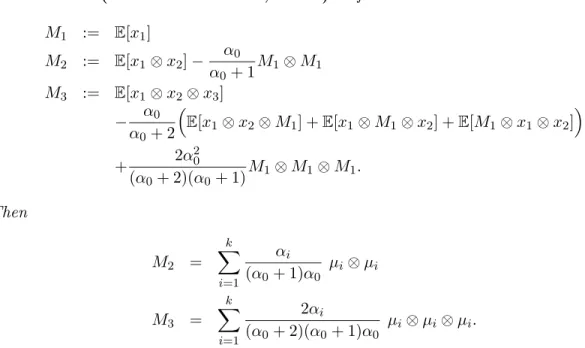
M1 := E[x1] M2 := E[x1⊗x2]− α0 α0+ 1 M1⊗M1 M3 := E[x1⊗x2⊗x3] − α0 α0+ 2 E[x1⊗x2⊗M1] +E[x1⊗M1⊗x2] +E[M1⊗x1⊗x2] + 2α 2 0 (α0+ 2)(α0+ 1) M1⊗M1⊗M1. Then M2 = k X i=1 αi (α0+ 1)α0 µi⊗µi M3 = k X i=1 2αi (α0+ 2)(α0+ 1)α0 µi⊗µi⊗µi.
Note that α0 needs to be known to form M2 and M3 from the raw moments. This, however, is a much weaker than assuming that the entire distribution of h is known (i.e., knowledge of the whole parameter vector α).
3.3 Multi-View Models
Multi-view models (also sometimes called na¨ıve Bayes models) are a special class of Bayesian networks in which observed variables x1, x2, . . . , xℓ are conditionally independent given a
latent variable h. This is similar to the exchangeable single topic model, but here we do not require the conditional distributions of the xt, t ∈ [ℓ] to be identical. Techniques
developed for this class can be used to handle a number of widely used models including hid-den Markov models (Mossel and Roch, 2006; Anandkumar et al., 2012c), phylogenetic tree models (Chang, 1996; Mossel and Roch, 2006), certain tree mixtures (Anandkumar et al., 2012b), and certain probabilistic grammar models (Hsu et al., 2012a).
As before, we leth∈[k] be a discrete random variable with Pr[h=j] =wj for allj∈[k].
Now consider random vectors x1 ∈ Rd1, x2 ∈ Rd2, and x3 ∈ Rd3 which are conditionally independent given h, and
E[xt|h=j] =µt,j, j∈[k], t∈ {1,2,3}
where theµt,j ∈Rdt are the conditional means of the xt given h =j. Thus, we allow the
observations x1, x2, . . . , xℓ to be random vectors, parameterized only by their conditional
means. Importantly, these conditional distributions may be discrete, continuous, or even a mix of both.
We first note the form for the raw (cross) moments.
Proposition 3.1 We have that:
E[xt⊗xt′] = k X i=1 wi µt,i⊗µt′,i, {t, t′} ⊂ {1,2,3}, t6=t′ E[x1⊗x2⊗x3] = k X i=1 wi µ1,i⊗µ2,i⊗µ3,i.
The cross moments do not possess a symmetric tensor form when the conditional distri-butions are different. Nevertheless, the moments can be “symmetrized” via a simple linear transformation of x1 and x2 (roughly speaking, this relates x1 and x2 to x3); this leads to an expression from which the conditional means of x3 (i.e., µ3,1, µ3,2, . . . , µ3,k) can be
recovered. For simplicity, we assume d1 = d2 = d3 =k; the general case (with dt ≥k) is
easily handled using low-rank singular value decompositions.
Theorem 3.6 (Anandkumar et al., 2012a) Assume that {µv,1, µv,2, . . . , µv,k} are lin-early independent for each v∈ {1,2,3}. Define
˜ x1 := E[x3⊗x2]E[x1⊗x2]−1x1 ˜ x2 := E[x3⊗x1]E[x2⊗x1]−1x2 M2 := E[˜x1⊗x˜2] M3 := E[˜x1⊗x˜2⊗x3]. Then M2 = k X i=1 wi µ3,i⊗µ3,i M3 = k X i=1 wi µ3,i⊗µ3,i⊗µ3,i.
We now discuss three examples (taken mostly from Anandkumar et al., 2012c) where the above observations can be applied. The first two concern mixtures of product distributions, and the last one is the time-homogeneous hidden Markov model.
3.3.1 Mixtures of Axis-Aligned Gaussians and Other Product Distributions
The first example is a mixture ofkproduct distributions inRnunder a mild incoherence as-sumption (Anandkumar et al., 2012c). Here, we allow each of thekcomponent distributions to have a different product distribution (e.g., Gaussian distribution with an axis-aligned co-variance matrix), but require the matrix of component means A:= [µ1|µ2| · · · |µk]∈Rn×k
to satisfy a certain (very mild) incoherence condition. The role of the incoherence condition is explained below.
For a mixture of product distributions, any partitioning of the dimensions [n] into three groups creates three (possibly asymmetric) “views” which are conditionally independent once the mixture component is selected. However, recall that Theorem 3.6 requires that for each view, the k conditional means be linearly independent. In general, this may not be achievable; consider, for instance, the case µi = ei for each i ∈ [k]. Such cases, where
the component means are very aligned with the coordinate basis, are precluded by the incoherence condition.
Define coherence(A) := maxi∈[n]{e⊤iΠAei}to be the largest diagonal entry of the
orthog-onal projector to the range ofA, and assumeAhas rankk. The coherence lies betweenk/n and 1; it is largest when the range ofAis spanned by the coordinate axes, and it isk/nwhen the range is spanned by a subset of the Hadamard basis of cardinality k. The incoherence condition requires, for someε, δ ∈(0,1), coherence(A)≤(ε2/6)/ln(3k/δ). Essentially, this condition ensures that the non-degeneracy of the component means is not isolated in just a few of the ndimensions. Operationally, it implies the following.
Proposition 3.2 (Anandkumar et al., 2012c) Assume A has rank k, and
coherence(A)≤ ε
2/6 ln(3k/δ)
for someε, δ∈(0,1). With probability at least1−δ, a random partitioning of the dimensions
[n] into three groups (for each i∈[n], independently pick t∈ {1,2,3} uniformly at random and put i in group t) has the following property. For each t ∈ {1,2,3} and j ∈ [k], let
µt,j be the entries of µj put into group t, and let At := [µt,1|µt,2| · · · |µt,k]. Then for each
t ∈ {1,2,3}, At has full column rank, and the k-th largest singular value of At is at least
p
(1−ε)/3 times that of A.
Therefore, three asymmetric views can be created by randomly partitioning the observed random vector x into x1, x2, and x3, such that the resulting component means for each view satisfy the conditions of Theorem 3.6.
3.3.2 Spherical Gaussian Mixtures, Revisited
Consider again the case of spherical Gaussian mixtures (cf. Section 3.2). As we shall see in Section 4.3, the previous techniques (based on Theorem 3.2 and Theorem 3.3) lead to estimation procedures when the dimension of xiskor greater (and when the kcomponent means are linearly independent). We now show that when the dimension is slightly larger, say greater than 3k, a different (and simpler) technique based on the multi-view structure can be used to extract the relevant structure.
We again use a randomized reduction. Specifically, we create three views by (i) applying a random rotation to x, and then (ii) partitioningx ∈Rn into three views ˜x1,x˜2,x˜3 ∈Rd for d := n/3. By the rotational invariance of the multivariate Gaussian distribution, the distribution of x after random rotation is still a mixture of spherical Gaussians (i.e., a mixture of product distributions), and thus ˜x1,x˜2,x˜3 are conditionally independent given h. What remains to be checked is that, for each viewt∈ {1,2,3}, the matrix of conditional means of ˜xt for each view has full column rank. This is true with probability 1 as long as
the matrix of conditional means A := [µ1|µ2| · · · |µk] ∈ Rn×k has rank k and n ≥ 3k. To
see this, observe that a random rotation in Rn followed by a restriction to dcoordinates is simply a random projection from Rn to Rd, and that a random projection of a linear subspace of dimension k to Rd is almost surely injective as long as d≥ k. Applying this observation to the range ofA implies the following.
Proposition 3.3 (Hsu and Kakade, 2013) Assume A has rank kand that n≥3k. Let
R ∈ Rn×n be chosen uniformly at random among all orthogonal n×n matrices, and set
˜
x:= Rx∈Rn and A˜:=RA= [Rµ1|Rµ2| · · · |Rµk]∈Rn×k. Partition [n] into three groups of sizes d1, d2, d3 with dt≥k for eacht∈ {1,2,3}. Furthermore, for eacht, definex˜t∈Rdt (respectively, A˜t ∈ Rdt×k) to be the subvector of x˜ (resp., submatrix of A˜) obtained by selecting the dt entries (resp., rows) in the t-th group. Then x˜1,x˜2,x˜3 are conditionally
independent given h; E[˜xt|h = j] = ˜Atej for each j ∈ [k] and t ∈ {1,2,3}; and with probability 1, the matrices A˜1,A˜2,A˜3 have full column rank.
It is possible to obtain a quantitative bound on thek-th largest singular value of eachAt
in terms of thek-th largest singular value of A(analogous to Proposition 3.2). One avenue is to show that a random rotation in fact causes ˜A to have low coherence, after which we can apply Proposition 3.2. With this approach, it is sufficient to require n = O(klogk) (for constant ε and δ), which results in the k-th largest singular value of each At being
a constant fraction of the k-th largest singular value of A. We conjecture that, in fact, n≥c·kfor somec >3 suffices.
3.3.3 Hidden Markov Models
Our last example is the time-homogeneous HMM for sequences of vector-valued observations x1, x2, . . . ∈ Rd. Consider a Markov chain of discrete hidden states y1 → y2 → y3 → · · · over kpossible states [k]; given a stateyt at timet, the observation xt at timet (a random
vector taking values in Rd) is independent of all other observations and hidden states. See Figure 1(b).
Letπ∈∆k−1 be the initial state distribution (i.e., the distribution ofy1), andT ∈Rk×k
be the stochastic transition matrix for the hidden state Markov chain: for all times t, Pr[yt+1=i|yt=j] =Ti,j, i, j∈[k].
Finally, letO ∈Rd×k be the matrix whosej-th column is the conditional expectation ofxt
given yt=j: for all times t,
Proposition 3.4 (Anandkumar et al., 2012c) Define h := y2, where y2 is the second hidden state in the Markov chain. Then
• x1, x2, x3 are conditionally independent given h;
• the distribution of h is given by the vector w:=T π∈∆k−1;
• for all j∈[k],
E[x1|h=j] =Odiag(π)T⊤diag(w)−1ej
E[x2|h=j] =Oej
E[x3|h=j] =OT ej.
Note the matrix of conditional means of xt has full column rank, for each t∈ {1,2,3},
provided that: (i) O has full column rank, (ii) T is invertible, and (iii) π and T π have positive entries.
4. Orthogonal Tensor Decompositions
We now show how recovering theµi’s in our aforementioned problems reduces to the
prob-lem of finding a certain orthogonal tensor decomposition of a symmetric tensor. We start by reviewing the spectral decomposition of symmetric matrices, and then discuss a generaliza-tion to the higher-order tensor case. Finally, we show how orthogonal tensor decomposigeneraliza-tions can be used for estimating the latent variable models from the previous section.
4.1 Review: The Matrix Case
We first build intuition by reviewing the matrix setting, where the desired decomposi-tion is the eigendecomposidecomposi-tion of a symmetric rank-k matrix M = VΛV⊤, where V =
[v1|v2| · · · |vk] ∈ Rn×k is the matrix with orthonormal eigenvectors as columns, and Λ =
diag(λ1, λ2, . . . , λk)∈Rk×k is diagonal matrix of non-zero eigenvalues. In other words,
M = k X i=1 λi viv⊤i = k X i=1 λi v⊗i 2. (1)
Such a decomposition is guaranteed to exist for every symmetric matrix.
Recovery of the vi’s and λi’s can be viewed at least two ways. First, each vi is fixed
under the mappingu7→M u, up to a scaling factor λi:
M vi = k X j=1 λj(v⊤jvi)vj =λivi as v⊤
jvi = 0 for all j 6=i by orthogonality. The vi’s are not necessarily the only such fixed
points. For instance, with the multiplicity λ1 =λ2 =λ, then any linear combination of v1 and v2 is similarly fixed underM. However, in this case, the decomposition in (1) is not unique, asλ1v1v⊤1 +λ2v2v2⊤is equal to λ(u1u⊤1 +u2u⊤2) for any pair of orthonormal vectors,
u1 and u2 spanning the same subspace as v1 and v2. Nevertheless, the decomposition is unique when λ1, λ2, . . . , λk are distinct, whereupon the vj’s are the only directions fixed
underu7→M u up to non-trivial scaling.
The second view of recovery is via the variational characterization of the eigenvalues. Assume λ1 > λ2 >· · · > λk; the case of repeated eigenvalues again leads to similar
non-uniqueness as discussed above. Then theRayleigh quotient
u7→ u
⊤M u
u⊤u
is maximized over non-zero vectors by v1. Furthermore, for any s∈[k], the maximizer of the Rayleigh quotient, subject to being orthogonal to v1, v2, . . . , vs−1, is vs. Another way
of obtaining this second statement is to consider the deflated Rayleigh quotient
u7→ u ⊤M−Ps−1 j=1λjvjv⊤j u u⊤u
and observe that vs is the maximizer.
Efficient algorithms for finding these matrix decompositions are well studied (Golub and van Loan, 1996, Section 8.2.3), and iterative power methods are one effective class of algorithms.
We remark that in our multilinear tensor notation, we may write the maps u 7→ M u and u7→u⊤M u/kuk2 2 as u7→M u ≡ u7→M(I, u), (2) u7→ u ⊤M u u⊤u ≡ u7→ M(u, u) u⊤u . (3)
4.2 The Tensor Case
Decomposing general tensors is a delicate issue; tensors may not even have unique decom-positions. Fortunately, the orthogonal tensors that arise in the aforementioned models have a structure which permits a unique decomposition under a mild non-degeneracy condition. We focus our attention to the case p = 3, i.e., a third order tensor; the ideas extend to generalp with minor modifications.
An orthogonal decomposition of a symmetric tensor T ∈ N3Rn is a collection of or-thonormal (unit) vectors{v1, v2, . . . , vk}together with corresponding positive scalarsλi >0
such that T = k X i=1 λivi⊗3. (4)
Note that since we are focusing on odd-order tensors (p = 3), we have added the require-ment that the λi be positive. This convention can be followed without loss of generality
since −λiv⊗i p = λi(−vi)⊗p whenever p is odd. Also, it should be noted that orthogonal
decompositions do not necessarily exist for every symmetric tensor.
In analogy to the matrix setting, we consider two ways to view this decomposition: a fixed-point characterization and a variational characterization. Related characterizations based on optimal rank-1 approximations are given by Zhang and Golub (2001).
4.2.1 Fixed-Point Characterization
For a tensorT, consider the vector-valued map
u7→T(I, u, u) (5) which is the third-order generalization of (2). This can be explicitly written as
T(I, u, u) = d X i=1 X 1≤j,l≤d Ti,j,l(e⊤ju)(e⊤lu)ei.
Observe that (5) isnot a linear map, which is a key difference compared to the matrix case. An eigenvector u for a matrix M satisfies M(I, u) =λu, for some scalar λ. We say a unit vector u∈Rn is aneigenvector of T, with correspondingeigenvalue λ∈R, if
T(I, u, u) =λu.
(To simplify the discussion, we assume throughout that eigenvectors have unit norm; oth-erwise, for scaling reasons, we replace the above equation with T(I, u, u) = λkuku.) This concept was originally introduced by Lim (2005) and Qi (2005). For orthogonally decom-posable tensorsT =Pki=1λiv⊗i 3, T(I, u, u) = k X i=1 λi(u⊤vi)2vi .
By the orthogonality of the vi, it is clear that T(I, vi, vi) = λivi for all i ∈[k]. Therefore
each (vi, λi) is an eigenvector/eigenvalue pair.
There are a number of subtle differences compared to the matrix case that arise as a result of the non-linearity of (5). First, even with the multiplicity λ1 = λ2 = λ, a linear combination u:=c1v1+c2v2 maynot be an eigenvector. In particular,
T(I, u, u) =λ1c21v1+λ2c22v2=λ(c21v1+c22v2)
may not be a multiple of c1v1+c2v2. This indicates that the issue of repeated eigenvalues does not have the same status as in the matrix case. Second, even if all the eigenvalues are distinct, it turns out that the vi’s are not the only eigenvectors. For example, set
u:= (1/λ1)v1+ (1/λ2)v2. Then,
T(I, u, u) =λ1(1/λ1)2v1+λ2(1/λ2)2v2=u,
sou/kuk is an eigenvector. More generally, for any subsetS⊆[k], the vector X
i∈S
1 λi ·
vi
As we now see, these additional eigenvectors can be viewed as spurious. We say a unit vector u is arobust eigenvector ofT if there exists anǫ >0 such that for all θ∈ {u′ ∈Rn:
ku′−uk ≤ǫ}, repeated iteration of the map ¯
θ7→ T(I,θ,¯ θ¯)
kT(I,θ,¯ θ¯)k , (6)
starting from θ converges to u. Note that the map (6) rescales the output to have unit Euclidean norm. Robust eigenvectors are also called attracting fixed points of (6) (see,e.g., Kolda and Mayo, 2011).
The following theorem implies that ifT has an orthogonal decomposition as given in (4), then the set of robust eigenvectors of T are precisely the set {v1, v2, . . . vk}, implying that
the orthogonal decomposition is unique. (For even order tensors, the uniqueness is true up to sign-flips of thevi.)
Theorem 4.1 Let T have an orthogonal decomposition as given in (4).
1. The set of θ ∈Rn which do not converge to some vi under repeated iteration of (6) has measure zero.
2. The set of robust eigenvectors of T is equal to {v1, v2, . . . , vk}.
The proof of Theorem 4.1 is given in Appendix A.1, and follows readily from simple or-thogonality considerations. Note that every vi in the orthogonal tensor decomposition is
robust, whereas for a symmetric matrixM, for almost all initial points, the map ¯θ7→ kMMθθ¯¯k converges only to an eigenvector corresponding to the largest magnitude eigenvalue. Also, since the tensor order is odd, the signs of the robust eigenvectors are fixed, as each −vi is
mapped tovi under (6).
4.2.2 Variational Characterization
We now discuss a variational characterization of the orthogonal decomposition. The gener-alized Rayleigh quotient (Zhang and Golub, 2001) for a third-order tensor is
u7→ T(u, u, u) (u⊤u)3/2 ,
which can be compared to (3). For an orthogonally decomposable tensor, the following theo-rem shows that a non-zero vectoru ∈Rnis anisolated local maximizer (Nocedal and Wright, 1999) of the generalized Rayleigh quotient if and only if u=vi for somei∈[k].
Theorem 4.2 Let T have an orthogonal decomposition as given in (4), and consider the optimization problem
max
u∈RnT(u, u, u) s.t. kuk ≤1.
1. The stationary points are eigenvectors of T.
2. A stationary point u is an isolated local maximizer if and only if u = vi for some
The proof of Theorem 4.2 is given in Appendix A.2. It is similar to local optimality anal-ysis for ICA methods using fourth-order cumulants (e.g., Delfosse and Loubaton, 1995; Frieze et al., 1996).
Again, we see similar distinctions to the matrix case. In the matrix case, the only local maximizers of the Rayleigh quotient are the eigenvectors with the largest eigenvalue (and these maximizers take on the globally optimal value). For the case of orthogonal tensor forms, the robust eigenvectors are precisely the isolated local maximizers.
An important implication of the two characterizations is that, for orthogonally decom-posable tensorsT, (i) the local maximizers of the objective functionu7→T(u, u, u)/(u⊤u)3/2 correspond precisely to the vectorsvi in the decomposition, and (ii) these local maximizers
can be reliably identified using a simple fixed-point iteration (i.e., the tensor analogue of the matrix power method). Moreover, a second-derivative test based on T(I, I, u) can be employed to test for local optimality and rule out other stationary points.
4.3 Estimation via Orthogonal Tensor Decompositions
We now demonstrate how the moment tensors obtained for various latent variable models in Section 3 can be reduced to an orthogonal form. For concreteness, we take the specific form from the exchangeable single topic model (Theorem 3.1):
M2 = k X i=1 wi µi⊗µi, M3 = k X i=1 wi µi⊗µi⊗µi.
(The more general case allows the weights wi in M2 to differ in M3, but for simplicity we keep them the same in the following discussion.) We now show how to reduce these forms to an orthogonally decomposable tensor from which the wi and µi can be recovered.
See Appendix D for a discussion as to how previous approaches (Mossel and Roch, 2006; Anandkumar et al., 2012c,a; Hsu and Kakade, 2013) achieved this decomposition through a certain simultaneous diagonalization method.
Throughout, we assume the following non-degeneracy condition.
Condition 4.1 (Non-degeneracy) The vectors µ1, µ2, . . . , µk∈Rd are linearly indepen-dent, and the scalars w1, w2, . . . , wk>0 are strictly positive.
Observe that Condition 4.1 implies that M2 0 is positive semidefinite and has rank k. This is often a mild condition in applications. When this condition is not met, learn-ing is conjectured to be generally hard for both computational (Mossel and Roch, 2006) and information-theoretic reasons (Moitra and Valiant, 2010). As discussed by Hsu et al. (2012b) and Hsu and Kakade (2013), when the non-degeneracy condition does not hold, it is often possible to combine multiple observations using tensor products to increase the rank of the relevant matrices. Indeed, this observation has been rigorously formulated in very recent works of Bhaskara et al. (2014) and Anderson et al. (2014) using the framework of smoothed analysis (Spielman and Teng, 2009).
4.3.1 The Reduction
First, letW ∈Rd×k be a linear transformation such that M2(W, W) = W⊤M2W = I
where I is the k×k identity matrix (i.e., W whitens M2). Since M2 0, we may for concreteness takeW :=U D−1/2, whereU ∈Rd×kis the matrix of orthonormal eigenvectors
of M2, andD∈Rk×k is the diagonal matrix of positive eigenvalues of M2. Let ˜ µi :=√wi W⊤µi. Observe that M2(W, W) = k X i=1 W⊤(√w iµi)(√wiµi)⊤W = k X i=1 ˜ µiµ˜⊤i = I,
so the ˜µi ∈Rk are orthonormal vectors.
Now define M3f :=M3(W, W, W)∈Rk×k×k, so that
f M3 = k X i=1 wi (W⊤µi)⊗3 = k X i=1 1 √w i ˜ µ⊗i3.
As the following theorem shows, the orthogonal decomposition of Mf3 can be obtained by identifying its robust eigenvectors, upon which the original parameters wi and µi can be
recovered. For simplicity, we only state the result in terms of robust eigenvector/eigenvalue pairs; one may also easily state everything in variational form using Theorem 4.2.
Theorem 4.3 Assume Condition 4.1 and take Mf3 as defined above.
1. The set of robust eigenvectors of Mf3 is equal to{µ˜1,µ˜2, . . . ,µ˜k}.
2. The eigenvalue corresponding to the robust eigenvector µ˜i of M3f is equal to 1/√wi, for all i∈[k].
3. If B ∈Rd×k is the Moore-Penrose pseudoinverse ofW⊤, and (v, λ) is a robust
eigen-vector/eigenvalue pair of Mf3, then λBv=µi for some i∈[k].
The theorem follows by combining the above discussion with the robust eigenvector charac-terization of Theorem 4.1. Recall that we have taken as convention that eigenvectors have unit norm, so theµi are exactly determined from the robust eigenvector/eigenvalue pairs of
f
M3 (together with the pseudoinverse ofW⊤); in particular, the scale of each µi is correctly
identified (along with the correspondingwi). Relative to previous works on moment-based
estimators for latent variable models (e.g., Anandkumar et al., 2012c,a; Hsu and Kakade, 2013), Theorem 4.3 emphasizes the role of the special tensor structure, which in turn makes transparent the applicability of methods for orthogonal tensor decomposition.
4.3.2 Local Maximizers of (Cross Moment) Skewness
The variational characterization provides an interesting perspective on the robust eigen-vectors for these latent variable models. Consider the exchangeable single topic models (Theorem 3.1), and the objective function
u7→ E[(x ⊤ 1u)(x⊤2u)(x⊤3u)] E[(x⊤ 1u)(x⊤2u)]3/2 = M3(u, u, u) M2(u, u)3/2 .
In this case, every local maximizer u∗ satisfies M2(I, u∗) = √wiµi for some i ∈ [k]. The
objective function can be interpreted as the (cross moment) skewness of the random vectors x1, x2, x3 along direction u.
5. Tensor Power Method
In this section, we consider the tensor power method of Lathauwer et al. (2000, Remark 3) for orthogonal tensor decomposition. We first state a simple convergence analysis for an orthogonally decomposable tensorT.
When only an approximation ˆT to an orthogonally decomposable tensor T is available (e.g., when empirical moments are used to estimate population moments), an orthogonal decomposition need not exist for this perturbed tensor (unlike for the case of matrices), and a more robust approach is required to extract the approximate decomposition. Here, we propose such a variant in Algorithm 1 and provide a detailed perturbation analysis. We note that alternative approaches such as simultaneous diagonalization can also be employed (see Appendix D).
5.1 Convergence Analysis for Orthogonally Decomposable Tensors
The following lemma establishes the quadratic convergence of the tensor power method—
i.e., repeated iteration of (6)—for extracting a single component of the orthogonal decom-position. Note that the initial vector θ0 determines which robust eigenvector will be the convergent point. Computation of subsequent eigenvectors can be computed with deflation,
i.e., by subtracting appropriate terms fromT.
Lemma 5.1 LetT ∈N3Rnhave an orthogonal decomposition as given in (4). For a vector
θ0∈Rn, suppose that the set of numbers|λ1v⊤1θ0|,|λ2v2⊤θ0|, . . . ,|λkv⊤kθ0|has a unique largest
element. Without loss of generality, say |λ1v1⊤θ0| is this largest value and |λ2v2⊤θ0| is the
second largest value. For t= 1,2, . . ., let
θt := T(I, θt−1, θt−1) kT(I, θt−1, θt−1)k . Then kv1−θtk2 ≤ 2λ21 k X i=2 λ−i 2 · λ2v2⊤θ0 λ1v1⊤θ0 2t+1 .
To obtain all eigenvectors, we may simply proceed iteratively using deflation, executing the power method on T −Pjλjvj⊗3 after having obtained robust eigenvector / eigenvalue
pairs{(vj, λj)}.
Proof Let θ0, θ1, θ2, . . . be the sequence given by θ0 := θ0 and θt := T(I, θt−1, θt−1) for t ≥ 1. Let ci := vi⊤θ0 for all i ∈ [k]. It is easy to check that (i) θt = θt/kθtk, and
(ii) θt = Pki=1λ2 t −1 i c2 t i vi. (Indeed, θt+1 = Pki=1λi(vi⊤θt)2vi = Pki=1λi(λ2 t −1 i c2 t i )2vi = Pk i=1λ2 t+1−1 i c2 t+1 i vi.) Then 1−(v⊤ 1θt)2 = 1− (v⊤ 1θt)2 kθtk2 = 1− λ 2t+1−2 1 c2 t+1 1 Pk i=1λ2 t+1−2 i c2 t+1 i ≤ Pk i=2λ2 t+1−2 i c2 t+1 i Pk i=1λ2 t+1−2 i c2 t+1 i ≤λ21 k X i=2 λ−i 2· λ2c2 λ1c1 2t+1 .
Since λ1 > 0, we have v1⊤θt > 0 and hence kv1 −θtk2 = 2(1−v⊤1θt) ≤ 2(1−(v⊤1θt)2) as
required.
5.2 Perturbation Analysis of a Robust Tensor Power Method
Now we consider the case where we have an approximation ˆT to an orthogonally decom-posable tensor T. Here, a more robust approach is required to extract an approximate decomposition. We propose such an algorithm in Algorithm 1, and provide a detailed per-turbation analysis. For simplicity, we assume the tensor ˆT is of size k×k×k as per the reduction from Section 4.3. In some applications, it may be preferable to work directly with a n×n×n tensor of rankk≤n(as in Lemma 5.1); our results apply in that setting with little modification.
Algorithm 1 Robust tensor power method
input symmetric tensor ˜T ∈Rk×k×k, number of iterations L,N.
output the estimated eigenvector/eigenvalue pair; the deflated tensor.
1: forτ = 1 to Ldo
2: Draw θ(0τ) uniformly at random from the unit sphere inRk.
3: for t= 1 to N do
4: Compute power iteration update
θt(τ) := ˜ T(I, θt(−τ)1, θ(t−τ)1) kT˜(I, θt(−τ)1, θ(t−τ)1)k (7) 5: end for 6: end for
7: Letτ∗ := arg max
τ∈[L]{T˜(θ(Nτ), θ
(τ)
N , θ
(τ)
N )}.
8: DoN power iteration updates (7) starting fromθN(τ∗)to obtain ˆθ, and set ˆλ:= ˜T(ˆθ,θ,ˆ θˆ).
Assume that the symmetric tensor T ∈Rk×k×kis orthogonally decomposable, and that ˆ
T =T+E, where the perturbationE ∈Rk×k×k is a symmetric tensor with small operator norm:
kEk:= sup kθk=1|
E(θ, θ, θ)|.
In our latent variable model applications, ˆT is the tensor formed by using empirical mo-ments, while T is the orthogonally decomposable tensor derived from the population mo-ments for the given model. In the context of parameter estimation (as in Section 4.3), E must account for any error amplification throughout the reduction, such as in the whitening step (see, e.g., Hsu and Kakade, 2013, for such an analysis).
The following theorem is similar to Wedin’s perturbation theorem for singular vectors of matrices (Wedin, 1972) in that it bounds the error of the (approximate) decomposition returned by Algorithm 1 on input ˆT in terms of the size of the perturbation, provided that the perturbation is small enough.
Theorem 5.1 Let Tˆ = T+E ∈Rk×k×k, where T is a symmetric tensor with orthogonal decomposition T =Pki=1λivi⊗3 where eachλi >0, {v1, v2, . . . , vk} is an orthonormal basis, andE is a symmetric tensor with operator normkEk ≤ǫ. Defineλmin:= min{λi :i∈[k]}, and λmax := max{λi :i ∈ [k]}. There exists universal constants C1, C2, C3 > 0 such that the following holds. Pick anyη ∈(0,1), and suppose
ǫ≤C1· λmin
k , N ≥C2·
log(k) + log logλmax ǫ , and s ln(L/log2(k/η)) ln(k) · 1− ln(ln(L/log2(k/η))) +C3 4 ln(L/log2(k/η)) − s ln(8) ln(L/log2(k/η)) ! ≥1.02 1 + s ln(4) ln(k) ! .
(Note that the condition on L holds with L= poly(k) log(1/η).) Suppose that Algorithm 1 is iteratively called k times, where the input tensor is Tˆ in the first call, and in each subsequent call, the input tensor is the deflated tensor returned by the previous call. Let
(ˆv1,ˆλ1),(ˆv2,λˆ2), . . . ,(ˆvk,λˆk) be the sequence of estimated eigenvector/eigenvalue pairs re-turned in these k calls. With probability at least 1−η, there exists a permutation π on [k]
such that kvπ(j)−ˆvjk ≤8ǫ/λπ(j), |λπ(j)−ˆλj| ≤5ǫ, ∀j ∈[k], and T − k X j=1 ˆ λjˆv⊗j3 ≤55ǫ.
The proof of Theorem 5.1 is given in Appendix B.
One important difference from Wedin’s theorem is that this is an algorithm dependent perturbation analysis, specific to Algorithm 1 (since the perturbed tensor need not have an
orthogonal decomposition). Furthermore, note that Algorithm 1 uses multiple restarts to ensure (approximate) convergence—the intuition is that by restarting at multiple points, we eventually start at a point in which the initial contraction towards some eigenvector dominates the error E in our tensor. The proof shows that we find such a point with high probability within L = poly(k) trials. It should be noted that for large k, the required bound onL is very close to linear ink.
We note that it is also possible to design a variant of Algorithm 1 that instead uses a stopping criterion to determine if an iterate has (almost) converged to an eigenvector. For instance, if ˜T(θ, θ, θ)>max{kT˜kF/√2r,kT˜(I, I, θ)kF/1.05}, where kT˜kF is the tensor
Frobenius norm (vectorized Euclidean norm), andris the expected rank of the unperturbed tensor (r =k−# of deflation steps), then it can be shown that θ must be close to one of the eigenvectors, provided that the perturbation is small enough. Using such a stopping criterion can reduce the number of random restarts when a good initial point is found early on. See Appendix C for details.
In general, it is possible, when run on a general symmetric tensor (e.g., ˆT), for the tensor power method to exhibit oscillatory behavior (Kofidis and Regalia, 2002, Example 1). This is not in conflict with Theorem 5.1, which effectively bounds the amplitude of these oscillations; in particular, if ˆT =T+E is a tensor built from empirical moments, the error term E (and thus the amplitude of the oscillations) can be driven down by drawing more samples. The practical value of addressing these oscillations and perhaps stabilizing the algorithm is an interesting direction for future research (Kolda and Mayo, 2011).
A final consideration is that for specific applications, it may be possible to use domain knowledge to choose better initialization points. For instance, in the topic modeling appli-cations (cf. Section 3.1), the eigenvectors are related to the topic word distributions, and many documents may be primarily composed of words from just single topic. Therefore, good initialization points can be derived from these single-topic documents themselves, as these points would already be close to one of the eigenvectors.
6. Discussion
In this section, we discuss some practical and application-oriented issues related to the tensor decomposition approach to learning latent variable models.
6.1 Practical Implementation Considerations
A number of practical concerns arise when dealing with moment matrices and tensors. Below, we address two issues that are especially pertinent to topic modeling applica-tions (Anandkumar et al., 2012c,a) or other settings where the observaapplica-tions are sparse.
6.1.1 Efficient Moment Representation for Exchangeable Models
In an exchangeable bag-of-words model, it is assumed that the words x1, x2, . . . , xℓ in a
document are conditionally i.i.d. given the topic h. This allows one to estimate p-th order moments using justpwords per document. The estimators obtained via Theorem 3.1 (single topic model) and Theorem 3.5 (LDA) use only up to third-order moments, which suggests that each document only needs to have three words.
In practice, one should use all of the words in a document for efficient estimation of the moments. One way to do this is to average over all ℓ3·3! ordered triples of words in a document of lengthℓ. At first blush, this seems computationally expensive (whenℓis large), but as it turns out, the averaging can be done implicitly, as shown by Zou et al. (2013). Let c ∈ Rd be the word count vector for a document of length ℓ, so ci is the number of
occurrences of wordiin the document, and Pdi=1ci =ℓ. Note thatcis a sufficient statistic
for the document. Then, the contribution of this document to the empirical third-order moment tensor is given by
1 ℓ 3 ·3!1 · c⊗c⊗c+ 2 d X i=1 ci (ei⊗ei⊗ei) − d X i=1 d X j=1 cicj (ei⊗ei⊗ej)− d X i=1 d X j=1 cicj (ei⊗ej⊗ei)− d X i=1 d X j=1 cicj (ei⊗ej ⊗ej) . (8)
It can be checked that this quantity is equal to 1 ℓ 3 · 1 3!· X
ordered word triple (x, y, z)
ex⊗ey⊗ez
where the sum is over all ordered word triples in the document. A similar expression is easily derived for the contribution of the document to the empirical second-order moment matrix: 1 ℓ 2 · 1 2!· c⊗c−diag(c) . (9) Note that the word count vectorcis generally a sparse vector, so this representation allows for efficient multiplication by the moment matrices and tensors in time linear in the size of the document corpus (i.e., the number of non-zero entries in the term-document matrix).
6.1.2 Dimensionality Reduction
Another serious concern regarding the use of tensor forms of moments is the need to op-erate on multidimensional arrays with Ω(d3) values (it is typically not exactly d3 due to symmetry). Whendis large (e.g., when it is the size of the vocabulary in natural language applications), even storing a third-order tensor in memory can be prohibitive. Sparsity is one factor that alleviates this problem. Another approach is to use efficient linear dimen-sionality reduction. When this is combined with efficient techniques for matrix and tensor multiplication that avoid explicitly constructing the moment matrices and tensors (such as the procedure described above), it is possible to avoid any computational scaling more than linear in the dimensiondand the training sample size.
Consider for concreteness the tensor decomposition approach for the exchangeable single topic model as discussed in Section 4.3. Using recent techniques for randomized linear algebra computations (e.g., Halko et al., 2011), it is possible to efficiently approximate the whitening matrix W ∈Rd×k from the second-moment matrix M2 ∈Rd×d. To do this, one first multiplies M2 by a random matrixR∈Rd×k′ for some k′≥k, and then computes the top k singular vectors of the product M2R. This provides a basis U ∈ Rd×k whose span
is approximately the range of M2. From here, an approximate SVD of U⊤M2U is used to
compute the approximate whitening matrixW. Note that both matrix productsM2R and U⊤M
2U may be performed via implicit access to M2 by exploiting (9), so that M2 need not be explicitly formed. With the whitening matrix W in hand, the third-moment tensor
f
M3 = M3(W, W, W) ∈ Rk×k×k can be implicitly computed via (8). For instance, the core computation in the tensor power method θ′ := Mf3(I, θ, θ) is performed by (i) computing η:=W θ, (ii) computingη′:=M3(I, η, η), and finally (iii) computingθ′ :=W⊤η′. Using the fact thatM3 is an empirical third-order moment tensor, these steps can be computed with O(dk+N) operations, where N is the number of non-zero entries in the term-document matrix (Zou et al., 2013).
6.2 Computational Complexity
It is interesting to consider the computational complexity of the tensor power method in the dense setting whereT ∈Rk×k×k is orthogonally decomposable but otherwise unstructured. Each iteration requires O(k3) operations, and assuming at most k1+δ random restarts for
extracting each eigenvector (for some smallδ >0) andO(log(k)+log log(1/ǫ)) iterations per restart, the total running time isO(k5+δ(log(k) + log log(1/ǫ))) to extract allkeigenvectors and eigenvalues.
An alternative approach to extracting the orthogonal decomposition ofT is to reorganize T into a matrix M ∈ Rk×k2 by flattening two of the dimensions into one. In this case, if T = Pki=1λiv⊗i 3, then M =
Pk
i=1λivi ⊗vec(vi ⊗vi). This reveals the singular value
decomposition ofM (assuming the eigenvaluesλ1, λ2, . . . , λkare distinct), and therefore can
be computed with O(k4) operations. Therefore it seems that the tensor power method is less efficient than a pure matrix-based approach via singular value decomposition. However, it should be noted that this matrix-based approach fails to recover the decomposition when eigenvalues are repeated, and can be unstable when the gap between eigenvalues is small— see Appendix D for more discussion.
It is worth noting that the running times differ by roughly a factor of Θ(k1+δ), which
can be accounted for by the random restarts. This gap can potentially be alleviated or removed by using a more clever method for initialization. Moreover, using special structure in the problem (as discussed above) can also improve the running time of the tensor power method.
6.3 Sample Complexity Bounds
Previous work on using linear algebraic methods for estimating latent variable models
cru-cially rely on matrix perturbation analysis for deriving sample complexity bounds (Mossel and Roch, 2006; Hsu et al., 2012b; Anandkumar et al., 2012c,a; Hsu and Kakade, 2013). The learning
algorithms in these works are plug-in estimators that use empirical moments in place of the population moments, and then follow algebraic manipulations that result in the desired parameter estimates. As long as these manipulations can tolerate small perturbations of the population moments, a sample complexity bound can be obtained by exploiting the conver-gence of the empirical moments to the population moments via the law of large numbers. As discussed in Appendix D, these approaches do not directly lead to practical algorithms