Graph Machine Learning
u
sing 3D Topological Models
Wassim Jabi
1, Abdulrahman Alymani
11
Cardiff University
Cardiff, United Kingdom
{jabiw, alymaniaa}@cardiff.ac.uk
ABSTRACT
Classification of urban and architectural works using machine learning techniques have typically focused on 2D pixel-based image recognition. In this paper we present a novel proof-of-concept workflow that enables a machine learning computer system to learn to classify 3D conceptual models based on topological graphs rather than 2D images. The system leverages two main technologies. The first is a custom designed software library that enhances the representation of 3D models through non-manifold topology and embedded semantic information. The second is an end-to-end deep graph convolutional network (DGCNN) that accepts graphs of an arbitrary structure without the need to first convert them into vectors. The experimental workflow consists of two stages. In the first stage, a generative parametric system was designed to create a large synthetic dataset of an urban block with several typological variations. The geometric models were then automatically labelled and converted into semantically rich topological dual graphs. In the second stage, the dual graphs were imported into the DGCNN for graph classification. Experiments demonstrate that the proposed workflow achieves accuracy results that are highly competitive with DGCNN’s classification of benchmark graph datasets.
Author Keywords
Machine Learning, Topological Models, Graphs.
ACM Classification Keywords
I.6.1 SIMULATION AND MODELING
1 INTRODUCTION
Understanding and classifying the typology of urban and architectural forms has been a topic of interest for a long period [19]. By understanding the typology of an urban form, relevant performative information can be extrapolated that helps urban designers and planners to make better decisions. Quantitative and statistical methods aided by computational tools have been shown to be effective in morphological studies [7]. While the impact of these approaches has thus far been limited in the mainstream practice of urban design and planning, there are signs that machine learning technologies (ML) are starting to revolutionize the recognition and classification of urban form. Several challenges still face the adoption of these technologies. First, supervised machine learning requires large datasets for training that are labelled. Second, most machine learning systems rely on 2D
pixel-based image recognition. While this may seem compatible with the representation of the available data – mainly city plans and drawings, this leads to major limitations. The urban environment is three-dimensional, topologically connected, and complex. However, most machine learning systems do not understand the semantics of the recognized image. To an ML algorithm, the data is simply a vector of mostly low resolution RGB values. If the data is 3D in nature and semantically rich, that information must be stripped away, and the data converted into images for an ML algorithm to operate properly. The lack of shareable 3D datasets is a real challenge and while some open-source sets do exist [9], their format, suitability, accessibility and licensing varies.
Even if 3D datasets are made available, there continues to be a challenge in recognizing and classifying them. Some researchers have focused on feature recognition of 3D models [12, 18]. These approaches capture several 2D snapshots of 3D models and match them to an image-based query, thus, still not fully capturing the three-dimensional and topological information embedded in the data. A slightly more sophisticated approach is to extract features from a 3D model and encode them as a vector to be used as input into a neural network [17]. This approach extracts only a portion of the data and must transform it into a standard input vector. It ignores the overall topological information that can be an indicator of the type of object.
A promising approach is to use machine learning on graphs [14, 16, 22]. The limitation of some approaches is that they decompose the graphs into small substructures such as walks or paths and derive the similarity between graphs based on a summation of attributes. The Deep Graph Convolutional Neural Network (DGCNN) avoids the above limitations and provides an end-to-end deep learning system for classifying graph-based data [26]. One of the main advantages of DGCNN is that it accepts arbitrary graphs without the need to first convert them into vectors.
Our aim in this paper is to design a novel proof-of-concept workflow that leverages DGCNN to classify 3D conceptual models based on their topological graphs rather than on their 2D representation. As a domain of investigation, we chose an urban block morphology. The workflow is divided into two stages. In the first stage, we use a software library, developed by one of the authors, that enhances the
representation of 3D models through non-manifold topology and embedded semantic information. The software is used to automatically and generatively create a large synthetic dataset of an urban block with several typological categories. The geometric models are then automatically labelled and converted into semantically rich topological graphs. In the second stage, we use this dataset as input to train DGCNN for graph classification.
The remainder of this paper is organised as follows: Section 2 briefly reviews related work carried out using graphs and machine learning in architecture. Section 3 provides a brief summary of Graphs theory. Section 4 describes the Topologic software library. Section 5 discusses related variations of Graph Convolutional Neural Networks (GCNN). Section 6 describes the Deep Graph Convolutional Neural Network (DGCNN) that was used for this research project. Section 7 details the experimental case study. Section 8 reports on the results of the experiments. Section 9 lists the limitations of this work. Finally, Section 10 provides concluding remarks and lists our plans for future work.
2 RELATED WORK
Beetz has researched the use of graph databases for harmonized distributed concept libraries for building information models [2]. His goal is to create “flexible, granular and cascading concept libraries for the building industry.” This work will enable standardization of the input data to graph neural networks. Tamke has researched the use of unsupervised and supervised machine learning approaches to deduce implicit information in building information models [20]. His platform can extract literal values, aggregates and derived values from IFC SPF files. Furthermore, the system possesses geometrical and topological analysis functionality that allows it to detect anomalies and to classify floor plans into two categories based on their geometrical appearance. Derix and Jagganath have researched methods to autonomously recognise spatial typologies through associations between spatial attributes of a layout [5]. They presented cases in which a building floor layout was analysed using space syntax concepts such as isovists, centrality and visual connectivity [10]. Their aim is to use these models to classify types and sequences of user experiences across buildings rather than strict typologies thus enabling an experience-based approach to architectural and urban design. Harding and Derix used a two-stage neural network and spectral graph theory as a spatial pattern recognition tool to develop a plan form of a reconfigurable exhibition space. To recognise and classify plans, they derived a graph using spatial adjacency and then reduced it by finding a “graph spectrum” which then forms a synaptic vector representation in feature space and thus “makes comparisons between graphs much easier to conduct.” What is interesting in their research is that they also use this approach for the automatic generation of spatial layouts. In their paper they describe a repulsion algorithm combined with a Voronoi diagram that distributes the graphs evenly
over the boundary plan. Topological connections are simulated as springs to maintain node adjacency.
3 GRAPHS
Explaining graph theory is beyond the scope of this paper, so a brief summary of its main concepts, data structures and metrics is provided here. For more detailed information on graph theory, please consult [23]. Graph theory is a branch of mathematics used to model relations between objects. A simple graph G consists of a set of points called vertices
V(G), and the lines that join pairs of points are called edges
E(G). The degree of a vertex in a graph is the number of edges connected to it. Vertices that are connected by an edge are called adjacent vertices. Similarly, edges that share a common vertex are called adjacent edges. Any two graphs that have a one-to-one correspondence between the number vertices, the number of edges and the degree of vertices are called isomorphic graphs.
4 TOPOLOGIC
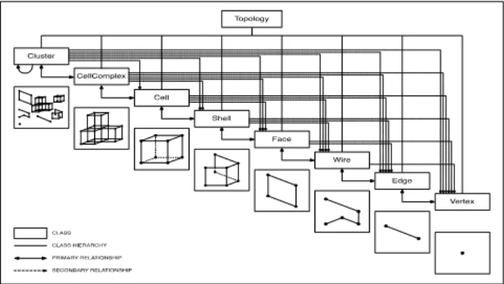
Topologic [21] is a 3D modelling software library developed by one of the authors that enhances the representation of space in 3D parametric and generative modelling environments such as Dynamo [6] and Grasshopper [8]. Topologic is based on the concept of non-manifold topology and has been described in [1, 11]. Topologic’s classes include: Vertex, Edge, Wire, Face, Shell, Cell, CellComplex, Cluster, Topology, Graph, Aperture, Content, and Context (see Figure 1). A Vertex is a point in 3D space with X, Y, Z coordinates. An Edge connects a start Vertex to an end Vertex. A Wire connects several Edges. A Face is made of a set of closed Wires. A Shell is a set of connected Faces that share Edges. A Cell is made from a closed Shell. A CellComplex is a set of connected Cells that share Faces. A Cluster is a grouping of topologies of any dimensionality. A Graph is a special data structure that is derived from Topologies. An Aperture is a special type of Face that is hosted by another Face. Any Topology can have additional Topologies added to its Contents. In turn, these Content Topologies will have a pointer back to their Context Topologies. This is similar to a parent/children relationship. In addition, any Topology can have a Dictionary that can hold any number of arbitrary key-attribute pairs.
In this paper, we will focus on two features of Topologic that were essential for the proposed workflow: 1) the automatic derivation of 3D topological dual graphs using the Cell, CellComplex, and Graph classes, and 2) the embedding of semantic information through custom dictionaries.
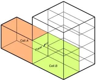
As mentioned above, In Topologic, a CellComplex is made of enclosed 3D spatial units (Cells) that share Faces. Cells that share Faces are called adjacent Cells (see Figure 2). The Graph class and associated methods are based on graph theory. A Graph is composed of Vertices and Edges that connect Vertices to each other. A Graph in Topologic accepts as input any Topology with additional optional parameters and outputs a Graph. In its simplest form, the dual graph of a CellComplex is a Graph that connects the centroids of adjacent Cells with a straight Edge (see Figure 3).
Figure 2. An example CellComplex. Cell A and Cell B are said to
be adjacent because they share Face F.
Figure 3. An example Dual Graph of the CellComplex. Each Cell is represented by a Vertex and the Vertices of adjacent Cells are
connected by an Edge.
A dictionary is a data structure made of key/value pairs. A key is any identifying string (e.g. “ID”, “Type”, “Name”). The value of a key can be of any data type (e.g.float, an integer, a string). Topologic enables the embedding of arbitrary dictionaries in any topology. As topologies undergo geometric operations (e.g. slicing a Cell into several smaller Cells thus creating a CellComplex), the dictionaries of operand topologies are transmitted to resulting topologies. Furthermore, when a dual graph is created from a Topology, the dictionaries of the constituent topologies get transferred to their corresponding vertices. We use this capability to label the vertices in the dual graph.
5 GRAPH CONVOLUTIONAL NETWORKS
Graph convolutional neural networks were first introduced by Bruna et al [3] where they demonstrated that it is possible to learn convolutional layers with a number of parameters independent of the input size, resulting in efficient deep architectures. In 2018, Xie and Grossman proposed a crystal graph convolutional neural network (CGCNN) that learns the properties of crystal atoms [24]. CGCNN offered highly accurate predictions of eight different properties of crystals. Chai et al proposed in 2018 a multi-graph convolutional neural network that can predict the bike flow at station-level in a bike sharing system [4]. Their model can outperform state-of-the-art prediction models by reducing the prediction error by up to 25.1%. Li et al proposed a Diffusion Convolutional Recurrent Neural Network (DCRNN), a deep learning framework for traffic forecasting that incorporates both spatial and temporal dependency in the flow of traffic [15]. Yu et al proposed graph convolutional networks to predict traffic speed in road systems that consistently outperforms state-of-the-art baselines on various real-world traffic datasets [25]. In 2019, Kipf and Welling introduced a scalable approach for learning on graph-structured data [13]. Their model scales linearly and can encode both local graph structures and features of nodes. They showed that their approach outperforms related methods by a significant margin on datasets in the domain of citation networks.
6 DEEP GRAPH CONVOLUTIONAL NETWORKS
In 2018, Zhang et al introduced an end-to-end deep-graph convolutional neural network (DGCNN) that accepts arbitrary graphs without the need to first convert them into tensors [26]. DGCNN accomplishes this by first passing the inputted graph through multiple graph convolution layers where node information is propagated between neighbours. Then a second layer sorts the graph vertices in a consistent order which are then inputted into a traditional convolutional neural network (see Figure 4). By sorting the vertex features rather than summing them up, DGCNN keeps far more information thus allowing it to learn from global graph topology. Furthermore, Zhang et al provide a theoretical proof that in DGCNN, if two graphs are isomorphic (i.e. have an identical structure), their graph representation after sorting the vertices is the same. This avoids the need to run additional costly algorithms to canonize the graph. Compared to state-of-the-art graph kernels, DGCNN has
Cell A
Cell B
Face
achieved highly competitive accuracy results on benchmark graph classification datasets.
Figure 4. The general structure of DGCNN (after Zhang et al [26]).
7 EXPERIMENTAL CASE STUDY
For the experimental case study, we created a workflow using Dynamo and Topologic that was designed to generate many 3D parametric models, and their associated topological dual graphs, of an urban block with a ground plate, an optional base that sits directly on top of the ground plate, and one or more tower blocks that sit either directly on the ground plate or directly on top of the base (see Figure 8).
Figure 5. The 3D model and dual graph in Autodesk Dynamo.
The ground plate can vary in size. The base is then dimensioned to be a certain percentage of the ground plate with equal offsets. One or several tower geometries are then placed with appropriate offsets and spacing. The height of the tower blocks is varied, but all tower blocks maintain the same height. Finally, the tower geometries are subdivided internally into a grid of Cells. This creates a 3D lattice structure. It is important to note that the internal sub-division of the tower block is to aid the neural network in distinguishing structures of different heights rather than to provide room-level detail.
To create the dataset, we needed to accomplish three tasks. The first task is to label the overall graph. We chose to limit
the classification of the graph to four categories: 1) Tower, 2) Slab, 3) Tower on Base, and 4) Slab on Base. The first classification (Tower) occurs when the base is not created, and the height of the tower is larger than its width and length. Similarly, a Slab classification occurs when the base is not created, but the height of the tower is less than or equal to its width and height. The last two categories repeat the rules of the first two but occur when a base is introduced.
The second task was to label the vertices. In addition to labelling the overall graph, DGCNN requires that each vertex in the graph is labelled. To experiment with the effect of labelling vertices, we created two separate datasets that contain the same graph topologies but with a different vertex labelling scheme. In the first dataset, called 3 labelled, we labelled vertices according to three categories: 1) Ground, 2) Base, and 3) Tower Cell. For the second dataset, called 5 labelled, we subdivided the tower cells into three categories based on their Z height value: 1) Low, 2) Medium, and 3) High. This yields five total labels: 1) Ground, 2) Base, 3) Low Tower Cell, 4) Medium Tower Cell, 5) High Tower Cell (see Figure 6).
Figure 6. Examples of auto-generated urban block configurations with associated dual graph.
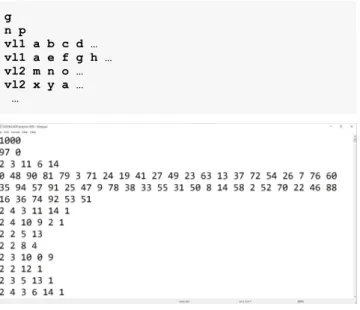
The last task was to integrate the visual dataflow definition with a custom python script to convert the 3D dual graph created by Topologic into a text file according to the format required by DGCNN (see Figure 7). The first line of the text file contains the total number of graphs (g). This is followed by g blocks of graphs where each block starts with a line that contains the number of vertices (n) followed by a number that indicates the classification (p) of that graph. This is then followed by a block of n vertices where each line starts with the label of the vertex (vl) followed by the indices of its adjacent vertices. The index of a vertex is implied by its line position using a zero-based numbering system.
g n p vl1 a b c d … vl1 a e f g h … vl2 m n o … vl2 x y a … …
Figure 7. The general dataset format required for DGCNN.
Since the dataset in synthetically produced through an iterative for loop, the resulting list is implicitly cyclical in complexity and height (see Figure 8). To avoid biased
training or the testing of only a specific level of complexity, the final list of graphs is reordered randomly.
The produced dataset totalled 1000 graphs as follows: 411 tower graphs
80 slab graphs
420 tower-on-base graphs 89 slab-on-base graphs
The total number of vertices is 292,570
The average number of vertices per graph is 292.57 The minimum number of vertices in a graph is 10 The maximum number of vertices in a graph is 1585 Tower graphs have an average of 399 vertices, minimum
of 37 vertices, and a maximum of 1,585 vertices Slab graphs have an average of 134 vertices, a minimum
of 19 vertices, and a maximum of 361 vertices
Tower-on-base graphs have an average of 259 vertices, a minimum of 14 vertices, and a maximum of 706 vertices Slab-on-base graphs have an average of 101 vertices, a minimum of 10 vertices, and a maximum of 433 vertices The reason towers-on-base and slabs-on-base have fewer vertices than those without a base is because they have a smaller footprint when placed on a base.
All experiments were implemented on an ordinary laptop computer running macOS Catalina 10.15 operating system with the following configuration: An Intel Core i7 Quad-Core CPU running at 2.7GHz with 16 GB of memory. DGCNN was deployed using the pytorch python environment.
For our experiments, we maintained most of the default values used by DGCNN. For details on these, please consult [26]. Below is a brief summary of these unmodified parameters:
Size of graphlets: 3.
Decay parameter: the largest power of 10 that is smaller than the reciprocal of the squared maximum node degree. SortingPool k: Set such that 60% of the graphs have
nodes more than k.
Two 1-D convolutional layers. The first layer has 16 output channels with a filter size of 2 and a step size of 2. The second 1-D convolutional layer has 32 output channels with a filter size of 5 and a step size of 1. The dense layer has 128 hidden units followed by a
softmax output layer.
A dropout layer is added at the end with a dropout rate of 0.5.
DGCNN uses a nonlinear hyperbolic function (tanh) in the graph convolution layers and a rectified linear units (ReLU) in the other layers. DGCNN does not use validation set labels for the training.
8 EXPERIMENTAL RESULTS
As detailed in the experimental results below, we varied only the following hyper-parameters: the training/testing ratio, the learning rate, the number of epochs, and the batch size.
8.1 Training and testing division ratio
The 1000 graphs in the two datasets were divided into training and testing data. We experimented with using 20%, 30% and 40% of the total graphs as testing data and then documented the resulting graph classification prediction accuracy (see Table 1). The 5 labelled dataset achieved consistently higher accuracy than the 3 labelled dataset. The highest accuracy (78.66%) was achieved for the 5 labelled dataset with a 30% testing ratio. Therefore, in subsequent experiments, we used this testing ratio to continue improving the accuracy of the results.
Training data
Testing data
% of
testing 3 Labelled 5 Labelled
800 graphs 200 graphs 20% 65.50% 69.00% 700 graphs 300 graphs 30% 64.45% 78.66% 600 graphs 400 graphs 40% 71.17% 72.00%
Table 1. Accuracy results using various training and testing ratios.
8.2 Learning rate
In convolutional neural networks, the learning rate is the amount by which the weights of nodes are updated during training. Varying the learning rate can dramatically affect the accuracy of the results. We experimented with four learning rates (1e-5, 1e-4, 1e-3, and 1e-2) and documented the results (see Table 2). A steep drop in the classification result was reported when using 1e-2 for both 3 labelled and 5 labelled datasets which was less than the acceptable rate. The highest
prediction accuracy result in this stage (79.66%) was achieved through a learning rate of 1e-4 on the 5 labelled dataset using a 30% testing ratio. This improved on the results achieved in the first round of testing. Therefore, in subsequent experiments, we used this testing ratio and learning rate to continue improving the accuracy of the results.
Learning Rate % of Testing 3 Labelled 5 Labelled
1e-5 30% 64.45% 78.66%
1e-4 30% 67.00% 79.66%
1e-3 30% 64.66% 67.00%
1e-2 30% 31.66% 34.66%
Table 2. Accuracy results using various learning rates.
8.3 Number of epochs
The number of epochs is the number of complete iterations through the training dataset. We experimented with various numbers of epochs while maintaining a testing rate of 1e-4 and a testing ratio of 30% (see Table 3). The best classification accuracy result was reported using 800 epochs for the 5 labelled dataset (84.33%). Exceeding that value (e.g. 1000 epochs) for the 5 labelled dataset resulted in a significant decrease in the classification accuracy which indicates that the model became over-fitted. The variation of the number of epochs for the 3 labelled dataset reported insignificant variation and was consistently worse than the accuracy reported for the 5 labelled dataset.
Number of epochs 3 Labelled 5 Labelled
500 67.00% 79.66%
800 67.33% 84.33%
1000 67.66% 78.66%
Table 3. Comparison of accuracy results using various epochs.
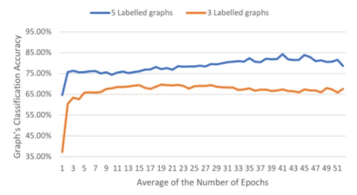
The line graph below charts the graphs’ classification accuracy for an average of 20 epochs (see Figure 9). The chart illustrates an elevated result for the 5 labelled dataset, with a moderate classification result for the 3 labelled dataset.
Figure 9. Learning rate and number of epochs for 3 labelled and 5 labelled datasets.
The 3 labelled model started learning and improved dramatically from the first few epochs. However, the accuracy level tapered after reaching approximately 220 epochs which means that the model stopped learning after that point. The 5 labelled model started learning well from the initial few epochs which began at approximately 65%. It then continued improving to reach a peak of 84.33%.
8.4 Batch size
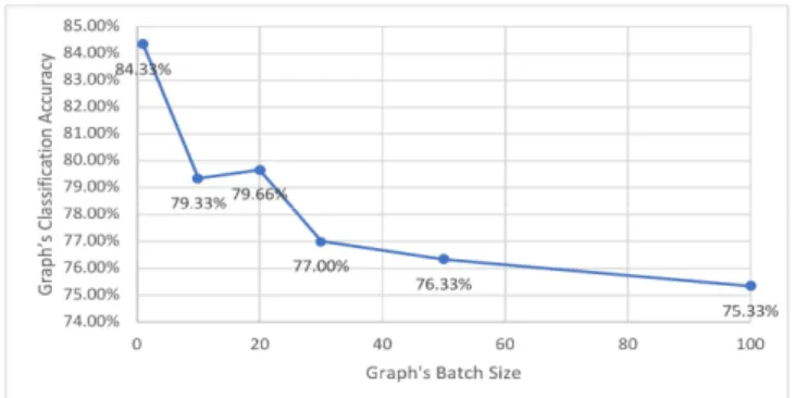
The batch size of gradient descent in convolutional neural networks controls the number of training samples to iterate through before the model’s internal parameters are updated. For this last experiment, we used the 1000 5 labelled dataset and maintained 30% testing ratio, 1e-4 learning rate and 800 epochs. We experimented with a diverse range of batch sizes (1, 10, 20, 30, 50 and 100). The best classification accuracy was reported for a batch size of 1 (see Table 4). However, a significant reduction in processing time (approximately 76%) can be achieved by increasing the batch size from 1 to 20 with a relatively modest loss in accuracy (approximately 5.5%). The associated line graph indicates the effect of the batch size on the classification accuracy (see Figure 10).
Batch size Accuracy Total Processing Time
1 84.33% 02:35:57 10 79.33% 00:36:30 20 79.66% 00:31:09 30 77.00% 00:31:22 50 76.33% 00:41:37 100 75:33% 01:09:50
Table 4. Comparison of accuracy results and total processing time using various batch sizes.
Figure 10. The effect of increasing the batch size on the
classification accuracy
9 LIMITATIONS
Due to the lack of ‘real’ datasets, we resorted to generating synthetic datasets based on parametric variation. Even if we were to obtain real datasets, they may need intervention and translation work to make them amenable for dual graph extraction. Furthermore, this paper focused on the domain of an urban block tower. Its applicability to other typologies remains to be tested in future work. We compared graphs with 3 labels and to ones with 5 labels and found the latter to
be more effective for machine learning. However, we do not know the effect of further increasing the number of labels, inventing a different labelling scheme, or using more complex topologies that represent further internal space division. By using a computer with moderate power, we were limited in the amount of training and testing that we could conduct. Finally, our workflow was tested and fine-tuned independently and was not compared to other approaches which may or may not be more effective.
10 CONCLUSION
In this paper we aimed to find out if we can classify urban form through a novel workflow that uses machine learning on three-dimensional graphs rather than on two-dimensional images. We leveraged a sophisticated topology-based 3D modelling environment to derive dual graphs from 3D models and label them automatically. We then fed those graphs to a state-of-the-art deep learning graph convolutional neural network. To discover the best accuracy rates, we experimented with the vertex labelling scheme, testing ratios, learning rates, number of epochs and number of batches.
At the conclusion of our experiments we found that the 5 labelled dataset of 1000 graphs with a testing ratio of 30%, a learning rate of 1e-4, using 800 epochs, and a batch size of 1 gave us the best prediction accuracy (84.33%). This result is highly competitive with accuracy results on benchmark datasets. Our approach shows strong promise for recognising urban and architectural forms using more semantically relevant and structured data. Planned future work will experiment with other datasets, labelling schemes, and will compare this novel workflow to other approaches.
We have identified several new areas of research based on our findings. First, we are planning to investigate node classification rather than just overall graph classification. Second, we are planning a system that may recognise the topological relationships the designer is building in near real-time and suggest precedents from a visual database. Other future planned work includes the use of this technique as a fitness function within an evolutionary algorithm to generate and evaluate urban block forms that fit within a context based on user’s preferences.
ACKNOWLEDGMENTS
The authors would like to thank Dr. Padraig Corcoran, Cardiff University for his help with graph neural networks and Mr. Akhil Meethal, ÉTS Montreal for his help with the
pytorch programming environment.
REFERENCES
1. Aish, R. et al. 2018. Topologic : Tools to explore architectural topology. Advances in Architectural Geometry 2018 (2018), 316–341.
2. Beetz, J. 2014. A Scalable Network of Concept Libraries Using Distributed Graph Databases.
Computing in Civil and Building Engineering. (2014), 955–1865.
3. Bruna, J. et al. 2014. Spectral networks and deep locally connected networks on graphs. 2nd International Conference on Learning
Representations, ICLR 2014 - Conference Track Proceedings (2014).
4. Chai, D. et al. 2018. Bike flow prediction with multi-graph convolutional networks. GIS: Proceedings of the ACM International Symposium on Advances in Geographic Information Systems. (2018), 397–400. DOI:https://doi.org/10.1145/3274895.3274896. 5. Derix, C. and Jagannath, P. 2014. Digital intuition –
Autonomous classifiers for spatial analysis and empirical design. The Journal of Space Syntax. 5, 2 (2014), 189–215.
6. Dynamo: http://dynamobim.org. Accessed: 2020-03-11.
7. Gil, J. et al. 2012. On the discovery of urban typologies: Data mining the many dimensions of urban form. Urban Morphology. 16, 1 (2012), 27–40. 8. Grasshopper 3D: http://grasshopper3d.com. Accessed:
2020-03-11.
9. Gröger, G. and Plümer, L. 2012. CityGML
-Interoperable semantic 3D city models. ISPRS Journal of Photogrammetry and Remote Sensing.
10. Hillier, B. and Hanson, J. 1984. The Social Logic of Space. Cambridge University Press.
11. Jabi, W. et al. 2018. Topologic: A toolkit for spatial and topological modelling. Computing for a Better Tomorrow, Proceedings of the 36th eCAADe conference (Lodz, Poland, 2018).
12. Kasaei, H. 2019. OrthographicNet: A Deep Learning Approach for 3D Object Recognition in Open-Ended Domains. (2019).
13. Kipf, T.N. and Welling, M. 2019. Semi-supervised classification with graph convolutional networks. 5th International Conference on Learning
Representations, ICLR 2017 - Conference Track Proceedings. (2019), 1–14.
14. Kriege, N. and Mutzel, P. 2012. Subgraph matching kernels for attributed graphs. Proceedings of the 29th International Conference on Machine Learning, ICML 2012. 2, (2012), 1015–1022.
15. Li, Y. et al. 2018. Diffusion convolutional recurrent neural network: Data-driven traffic forecasting. 6th International Conference on Learning
Representations, ICLR 2018 - Conference Track Proceedings. (2018), 1–16.
16. Orsini, F. et al. 2015. Graph invariant kernels. IJCAI International Joint Conference on Artificial
Intelligence. 2015-Janua, Ijcai (2015), 3756–3762. 17. Qin, F. et al. 2014. A deep learning approach to the
classification of. 15, 2 (2014), 91–106. DOI:https://doi.org/10.1631/jzus.C1300185. 18. Sarkar, K. et al. 2017. Trained 3d models for CNN
based object recognition. VISIGRAPP 2017 -Proceedings of the 12th International Joint Conference on Computer Vision, Imaging and Computer Graphics Theory and Applications. 5, (2017), 130–137.
DOI:https://doi.org/10.5220/0006272901300137. 19. Steadman, P. et al. 2000. A classification of built forms. Environment and Planning B: Planning and Design. (2000). DOI:https://doi.org/10.1068/bst7. 20. Tamke, M. 2015. Assessing implicit knowledge in
BIM models with machine learning. Modelling Behaviour. December (2015).
DOI:https://doi.org/10.1007/978-3-319-24208-8. 21. Topologic: 2019. https://topologic.app. Accessed:
2020-03-14.
22. Vishwanathan, S.V.N. et al. 2010. Graph kernels.
Journal of Machine Learning Research. 11, (2010), 1201–1242. DOI:https://doi.org/10.1007/978-0-387-30164-8_349.
23. Voloshin, V.I. 2009. Introduction to graph theory. 24. Xie, T. and Grossman, J.C. 2018. Crystal Graph
Convolutional Neural Networks for an Accurate and Interpretable Prediction of Material Properties.
Physical Review Letters. 120, 14 (2018).
DOI:https://doi.org/10.1103/PhysRevLett.120.145301. 25. Yu, B. et al. 2018. Spatio-temporal graph
convolutional networks: A deep learning framework for traffic forecasting. IJCAI International Joint Conference on Artificial Intelligence. 2018-July, (2018), 3634–3640.
DOI:https://doi.org/10.24963/ijcai.2018/505. 26. Zhang, M. et al. 2018. An end-to-end deep learning
architecture for graph classification. 32nd AAAI Conference on Artificial Intelligence, AAAI 2018. (2018), 4438–4445.