A General Framework for Multi-fidelity Bayesian Optimization with Gaussian Processes

(1)

A General Framework for Multi-fidelity Bayesian

Optimization with Gaussian Processes

California Institute of Technology Pasadena, CA, USA

Abstract

How can we efficiently gather information to optimize an unknown function, when pre-sented with multiple, mutually dependent information sources with different costs? For example, when optimizing a robotic system, intelligently trading off computer simulations and real robot testings can lead to significant savings. Existing methods, such as multi-fidelity GP-UCB or Entropy Search-based approaches, either make simplistic assumptions on the interaction among different fidelities or use simple heuristics that lack theoretical guarantees. In this paper, we study multi-fidelity Bayesian optimization with complex structural dependencies among multiple outputs, and proposeMF-MI-Greedy, a principled algorithmic framework for addressing this problem. In particular, we model different fideli-ties using additive Gaussian processes based on shared latent structures with the target function. Then we use cost-sensitive mutual information gain for efficient Bayesian global optimization. We propose a simple notion of regret which incorporates the cost of different fidelities, and prove that MF-MI-Greedy achieves low regret. We demonstrate the strong empirical performance of our algorithm on both synthetic and real-world datasets.

1. Introduction

Optimizing an unknown function that is expensive to evaluate is a common problem in real applications. Examples include experimental design for protein engineering, where chemists need to synthesize designed amino acid sequences and then test whether they satisfy certain properties (Romero et al., 2013); or black-box optimization for material science, where scientists need to run extensive computational experiments at various levels of accuracy to find the optimal material design structure (Fleischman et al., 2017). Conducting real experiments could be labor-intensive and time-consuming. In practice, we would like to look for alternative ways to gather information so that we can make the most effective use of real experiments that we do conduct. A natural candidate is computer simulation (van Gunsteren & Berendsen, 1990), which tends to be less time consuming but produces less accurate results. For example, computer simulation is ubiquitous in robotic applications,

(2)

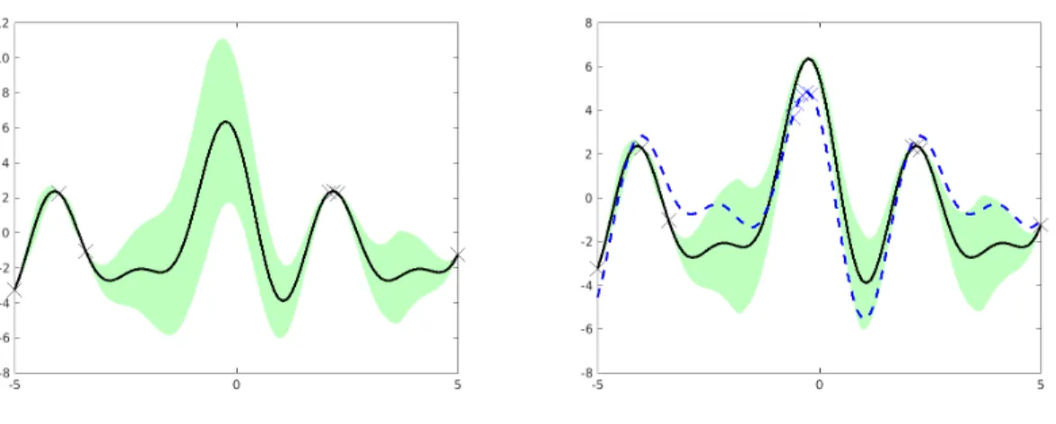
(a) Only querying target fidelity function. (b) Querying both target and a lower fidelity.

Figure 1: Benefit from multi-fidelity Bayesian optimization. The left panel shows normal single fidelity Bayesian optimization where locations near a query point (crosses) have low uncertainty. When there is a lower fidelity cheaper approximation in the right panel, by querying a large number of points of the lower fidelity function, the uncertainty in the target fidelity can also be reduced significantly.

e.g. we test a control policy first in simulation before deploying it in a real physical system (Marco et al.,2017).

The central challenge in efficiently using multiple sources of information is captured in the general framework of multi-fidelity optimization (Forrester et al.,2007;Kandasamy et al.,2016,2017;Marco et al.,2017;Sen et al.,2018) where multiple functions with varying degrees of accuracy and costs can be effectively leveraged to provide the maximal amount of information. However, strict assumptions, such as requiring strict relations between the quality and the cost of a lower fidelity function, and two-stage query selection criteria (cf. §2.2) are likely to limit their practical use and lead to sub-optimal selections.

In this paper, we propose a general and principled multi-fidelity Bayesian optimization frameworkMF-MI-Greedy (Multi-fidelity Mutual Information Greedy) that prioritizes max-imizing the amount of mutual information gathered across fidelity levels. Figure1captures the intuition of maximizing mutual information. Gathering information from lower fidelity also conveys information on the target fidelity. We make this idea concrete in §4. Our method improves upon prior work on multi-fidelity Bayesian optimization by establishing explicit connections across fidelity levels to enable joint posterior updates and hyperparam-eter optimization. In summary, our contributions in this paper are

• We study multi-fidelity Bayesian optimization with complex structural dependencies among multiple outputs (§3), and propose MF-MI-Greedy, a principled algorithmic framework for addressing this problem (§4).

• We propose a simple notion of regret which incorporates the cost of different fidelities, and prove thatMF-MI-Greedy achieves low regret (§5).

• We demonstrate the empirical performance of MF-MI-Greedy on both simulated and real-world datasets (§6).

(3)

2. Background and Related Work

In this section, we review related work on Bayesian optimization with Gaussian processes.

2.1 Background on Gaussian Processes

Gaussian process (Rasmussen & Williams, 2006) models an infinite collection of random variables, each indexed by an x ∈ X, such that every finite subset of random variables has a multivariate Gaussian distribution. The GP distribution GP (µ(x), k(x, x0)) is a joint Gaussian distribution over all those (infinitely many) random variables specified by its mean

µ(x) =E[f(x)] and covariance (also known as kernel) function

k(x, x0) =E(f(x)−µ(x)) f(x0)−µ(x0).

A key advantage of GP is that it is very efficient to perform inference. Assume thatf ∼ GP (µ(x), k(x, x0)) is a sample from the GP distribution, and thaty=f(x) +ε(x) is a noisy observation of the function valuef(x). Here, the noiseε(x)∼ N(0, σ2(x)) could depend on the input x. Suppose that we have selected S ⊆ X and received yS = [f(xi) +ε(xi)]xi∈S.

We can obtain the posterior mean µS(x) and covariance kS(x, x0) of the function through the covariance matrix KS = [k(xi, xj) +δijσ2(xi)]xi,xj∈S and kS(x) = [k(xi, x)]xi∈S:

µS(x) =µ(x) +kS(x)|K_S−1yS (1)

kS(x, x0) =k(x, x0)−kS(x)|K_S−1kS(x0) (2) whereδij is the Kronecker delta function.

2.2 Bayesian Optimization via Gaussian Processes

Single-fidelity Gaussian Process optimization Optimizing an unknown and noisy function is a common task in Bayesian optimization. In real applications, such functions tend to be expensive to evaluate, for example tuning hyperparameters for deep learning models (Snoek et al., 2012), so the number of queries should be minimized. As a way to model the unknown function, Gaussian process (GP) (Rasmussen & Williams, 2006) is an expressive and flexible tool to model a large class of functions. A classical method for Bayesian optimization with GPs is GP-UCB (Srinivas et al., 2010) which treats Bayesian optimization as a multi-armed bandit problem and proposes an upper-confidence bound based algorithm for query selections. The authors provide a theoretical bound on the cumulative regret that is connected with the amount of mutual information gained through the queries. (Contal et al., 2014) directly incorporates mutual information into the UCB framework and demonstrated the empirical value of their method.

Entropy search (Hennig & Schuler,2012) represents another class of GP-based Bayesian optimization approach. Its main idea is to directly search for the global optimum of an unknown function through queries. Each query point is selected based on its informativeness in learning the location for the function optimum. Predictive entropy search (Hern´ andez-Lobato et al.,2014) addresses some computational issues from entropy search by maximizing the expected information gain with respect to the location of the global optimum. Max-value entropy search (Wang et al., 2016; Wang & Jegelka, 2017) approaches the task of

(4)

searching the global optimum differently. Instead of searching for the location of the global optimum, it looks for the value of the global optimum. This effectively avoids issues related to the dimension of the search space and the authors are able to provide regret bound analysis that the previous two entropy search methods lack.

A computational consideration for learning with GPs concerns with optimizing specific kernels used to model the covariance structures of GPs. As this optimization task de-pends on the dimension of feature space, approximation methods are needed to speed up the learning process. Random Fourier features (Rahimi & Recht,2008) are efficient tools for dimension reduction and are employed in GP regression tasks (L´azaro-Gredilla et al.,

2010). As elaborated on in §4, our algorithmic framework offers the flexibility of choosing among different single-fidelity optimization approaches as a subroutine, so that one can take advantage of these computational and approximation algorithms for efficient optimization.

Multi-output Gaussian Process Sometimes it is desirable to model multiple corre-lated outputs with Gaussian processes. Most GP-based multi-output models create cor-related outputs by mixing a set of independent latent processes. A simple form of such a mixing scheme is the linear model of coregionalization (Teh et al., 2005; Bonilla et al.,

2008) where each output is modeled as a linear combination of latent GPs with fixed coef-ficients. The dependencies among outputs are captured by sharing those latent GPs. More complex structures can be captured by a linear combination of GPs with input-dependent coefficients (Wilson et al., 2012), shared inducing variables (Nguyen & Bonilla, 2014), or convolved process (Boyle & Frean,2005; Alvarez & Lawrence, 2009). In comparison with single fidelity/output GPs, multi-output GP often requires more sophisticated approximate models for efficient optimization (e.g., using inducing points (Snelson & Ghahramani,2007) to reduce the storage and computational complexity, and variational inference approaches to approximate the posterior of the latent processes (Titsias,2009;Nguyen & Bonilla,2014)). While the analysis of our framework is not limited to a fixed structural assumption in modeling the joint distribution among multiple outputs, for efficiency concern, we use a simple, additive model between multiple fidelity outputs in our experiments (cf. §6.1) to demonstrate the effectiveness of the optimization framework.

Multi-fidelity Bayesian optimization Multi-fidelity optimization is a general frame-work that captures the trade-off between cheap low quality and expensive high quality data. Recently, there have been several works on using GPs to model functions of different fidelity levels. Recursive co-kriging (Forrester et al., 2007; Le Gratiet & Garnier, 2014) consider an autoregressive model for multi-fidelity GP regression, which assumes that the higher fidelity consists of a lower fidelity term and an independent GP term which models the systematic error for approximating the higher-fidelity output. Therefore, one can model cross-covariance between the high-fidelity and low-fidelity functions using the covariance of the lower fidelity function only. Virtual vs Real (Marco et al., 2017) extends this idea to Bayesian optimization. The authors consider a two-fidelity setting (i.e., virtual sim-ulation and real system experiments), where they model the correlation between the two fidelities through co-kriging, and then apply entropy search (ES) to optimize the target out-put. Zhang et al.(2017) model the dependencies between different fidelities with convolved Gaussian processes (Alvarez & Lawrence,2009), and then apply predictive entropy search (PES) (Hern´andez-Lobato et al.,2014) to efficient exploration. Although both the ES and

(5)

multi-fidelity PES heuristics have shown promising empirical results on some datasets, little is known about their theoretical performance.

Recently, Kandasamy et al. (2016) proposed Multi-fidelity GP-UCB (MF-GP-UCB), a principled framework for multi-fidelity Bayesian optimization with Gaussian processes. In a followup work (Kandasamy et al.,2017;Sen et al.,2018), the authors address the disconnect issue by considering a continuous fidelity space and performing joint updates to effectively share information among different fidelity levels.

In contrast to our general assumption on the joint distribution between different fideli-ties,Kandasamy et al.(2016) andSen et al.(2018) assume a specific structure over multiple fidelities, where the cost of each lower fidelity is determined according to the maximal ap-proximation error in function value when compared with the target fidelity. Kandasamy et al. (2017) consider a two-stage optimization process, where the action and the fidelity level are selected in two separate stages. We note that this procedure may lead to non-intuitive choices of queries: For example, in a pessimistic case where the low fidelity only differs from the target fidelity by a constant shift, their algorithm is likely to focus only on querying the target fidelity actions even though the low fidelity is as useful as the target fidelity. In contrast, as described in §4, our algorithm jointly selects a query point and a fidelity level so such sub-optimality can be avoided.

3. Problem Statement

We now introduce useful notations and formally state the problem studied in this paper.

Payoff function and auxiliary functions Consider the problem of maximizing an un-known payoff functionfm:X →R. We can probe the functionfmby directly querying it at somex∈ X and obtaining a noisy observationyhx,mi=fm(x) +ε(x), whereε(x)∼ N(0, σ2) denotes i.i.d. Gaussian white noise. In addition to the payoff functionfm, we are also given access to oracle calls to some unknown auxiliary functions f1, . . . , fm−1 :X →R; similarly, we obtain a noisy observationyhx,`i=f`(x) +εwhen querying f` atx. Here, each f` could be viewed as a low-fidelity version of fm for ` < m. For example, if fm(x) represents the actual reward obtained by running a real physical system with input x, then f`(x) may represent the simulated payoff from a numerical simulator at fidelity level `.

Joint distribution on multiple fidelities We assume that multiple fidelities{f`}`∈[m]

are mutually dependent through some fixed, (possibly) unknown joint probability distri-bution P[f1, . . . , fm]. In particular, we modelP with a multiple output Gaussian process; hence the marginal distribution on each fidelity is a separate GP, i.e., ∀` ∈ [m], f` ∼ GP (µ`(x), k`(x, x0)), whereµ`, k` specify the (prior) mean and covariance at fidelity level`.

Action, reward, and cost Let us use hx, `i to denote the action of querying f` at x. Each action hx, `iincurs a cost of λ`, and achieves a reward

q(hx, `i) =

(

fm(x) if`=m qmin o.w.

(3)

That is, performing hx, mi (at the target fidelity) achieves a reward fm(x). We receive the minimal immediate rewardqmin with lower fidelity actions hx, `i for ` < m, even though it

(6)

may provide some information aboutfm and could thus lead to more informed decisions in the future. W.l.o.g., we assume that maxxfm(x)≥0, andqmin≡0.

Policy Let us encode an adaptive strategy for picking actions as a policyπ. In words, a policy specifies which action to perform next, based on the actions picked so far and the corresponding observations. We consider policies with a fixed budget Λ. Upon termination,

π returns a sequence of actionsSπ, such thatP

hx,`i∈Sπλ` ≤Λ. Note that for a given policy

π, the sequence S_π is random, dependent on the joint distribution P and the (random) observations of the selected actions.

Objective Given a budget Λ on π, our goal is to maximize the expected cumulative reward, so as to identify an actionhx, mi with performance close tox∗= maxx∈Xfm(x) as rapidly as possible. Formally, we seek

π∗ = arg max π:P hx,ì∈Sπλ`≤Λ ESπ   X hx,ì∈Sπ q(hx, ì)   (4)

Remarks Problem 4 strictly generalizes the optimal value of information (VoI) problem (Chen et al.,2015) to the online setting. To see this, consider the scenario where λm λ` for` < m, and Λ∈(λm,2λm). To achieve a non-zero reward, a policy must pickhx, mi as the last action before exhausting the budget Λ. Therefore, our goal becomes to adaptively pick lower fidelity actions that are the most informative about x∗ under budget Λ−λm, which reduces to the optimal VoI problem.

4. The Multi-fidelity BO Framework

We now presentMF-MI-Greedy, a general framework for multi-fidelity Gaussian process op-timization. In a nutshell,MF-MI-Greedy attempts to balance the “exploratory” low-fidelity actions and the more expensive target fidelity actions, based on how much information (per unit cost) these actions could provide about the target fidelity function. Concretely, MF-MI-Greedy proceeds in rounds under a given budget Λ. Each round can be divided into two phases: (i) an exploration (i.e., information gathering) phase, where the algorithm focuses on exploring the low fidelity actions, and (ii) an optimization phase, where the algorithm tries to optimize the payoff functionfmby performing an actionhx, miat the target fidelity. The pseudo-code of the algorithm is provided in Algorithm 1.

Exploration phase A key challenge in designing the algorithm is to decide when to stop exploration (or equivalently, to invoke the optimization phase). Note that this is analogous to the exploration-exploitation dilemma in the classical single-fidelity Bayesian optimization problems; the difference is that in the multi-fidelity setting, we have a more distinctive notion of “exploration”, and a more complicated structure of the action space (i.e., each exploration phase corresponds to picking a set of low fidelity actions). Furthermore, note that there is no explicit measurement of the relative “quality” of a low fidelity action, as they all have uniform reward by our modeling assumption (c.f. Eq. (3)); hence we need to design a proper heuristic to keep track of the progress of exploration.

We consider an information-theoretic selection criterion for picking low fidelity actions. The quality of a low fidelity action hx, `i is captured by the information gain, defined as

(7)

Algorithm 1: Multi-fidelity Mutual Information Greedy Optimization ( MF-MI-Greedy)

1 Input: Total budget Λ; cost λi for all fidelitiesi∈[m]; joint GP (prior) distribution on{fi, εi}i∈[m]

begin

2 S ← ∅

3 B←Λ ; /* initialize remainig budget */

whileB >0 do

/* explore with low fidelity */

4 L ←Explore-LF B,[λ_`],GP {f_`, ε_`}_`_∈_[_m_],S

/* select target fidelity */

5 x∗ ←SF-GP-OPT(GP ({fm, εm}),yS∪L) 6 S ← S ∪ L ∪ {hx∗, mi}

7 B←Λ−ΛS ; /* update remaining budget */

8 Output: Optimizer of the target functionf_m

the amount of entropy reduction in the posterior distribution of the target payoff function1_: I yhx,ì;fm y_S =H yhx,ì y_S −_H yhx,ì f_m,y_S

. Here,S denotes the set of previously selected actions, and yS denote the observation history. Given an exploration budget B, our objective for a single exploration phase is to find a set of low-fidelity actions, which are (i) maximally informative about the target function, (ii) better than the best action on the target fidelity when considering the information gain per unit cost (otherwise, one would rather pick the target fidelity action to trade off exploration and exploitation), and (iii) not overly aggressive in terms of exploration (since we would also like to reserve a certain budget for performing target fidelity actions to gain reward).

Finding the optimal set of actions satisfying the above design principles is computa-tionally prohibitive, as it requires us to search through a combinatorial (for finite discrete domains) or even infinite (for continuous domains) space. In Algorithm 2, we introduce Explore-LF, a key subroutine of MF-MI-Greedy, for efficient exploration on low fidelities. At each step, Explore-LF takes a greedy step w.r.t. the benefit-cost ratio over all actions. To ensure that the algorithm does not explore excessively, we consider the following stopping conditions: (i) when the budget is exhausted (Line 6), (ii) when a single target fidelity action is better than all the low fidelity actions in terms of the benefit-cost ratio (Line 7), and (iii) when the cumulative benefit-cost ratio is small (Line 8). Here, the parameter β is set to be Ω√1

B

to ensure low regret, and we defer the detailed discussion of the choice of β to§5.2.

Optimization phase At the end of the exploration phase, MF-MI-Greedy updates the posterior distribution of the joint GP using the full observation history, and searches for a target fidelity action via the (single-fidelity) GP optimization subroutine SF-GP-OPT (Line 5). Here, SF-GP-OPT could be any off-the-shelf Bayesian optimization algorithm, 1. An alternative, more aggressive information measurement is the information gain over theoptimizer of

the target functionfm(Hennig & Schuler,2012), i.e.,I yhx,`i; arg maxxfm(x)

yS

, or theoptimal value offm(Wang & Jegelka,2017), i.e.,I yhx,`i; maxxfm(x)

yS.

(8)

Algorithm 2:Explore-LF: Explore low fidelities

1 Input: Exploration budgetB; cost [λ`]_`∈[m]; joint GP distribution on{fi, εi}i∈[m];

previously selected itemsS

begin

2 L ← ∅; /* selected actions */

3 ΛL←0 ; /* cost of selected actions */

4 β← _α₍1_B₎ ; /* threshold (c.f. Theorem 4) */

whiletrue do

/* greedy benefit-cost ratio */

5 hx∗, `∗i ←arg max_h_x,`_i_:_λ

`≤B−ΛL−λm

I(yhx,`i;fm|yS∪L)

λ`

if `∗=nullthen

6 break ; /* budget exhausted */

if `∗=mthen

7 break ; /* worse than target */

else if I(yL∪{hx∗,`∗i};fm|yS)

(ΛL+λ`∗) < βthen

8 break ; /* low cumulative ratio */

else

9 L ← L ∪ {hx∗, `∗i} 10 ΛL←ΛL+λ`∗

11 Output: Selected set of itemsL from lower fidelities

such as GP-UCB (Srinivas et al., 2010), GP-MI (Contal et al., 2014), EST (Wang et al.,

2016) and MVES (Wang & Jegelka, 2017), etc. Different from the previous exploration phase which seeks an informative set of low fidelity actions, the GP optimization subroutine aims to trade off exploration and exploitation on the target fidelity, and outputs a single action at each round. MF-MI-Greedy then proceeds to the next round until it exhausts the preset budget and eventually outputs an estimator of the target function optimizer.

5. Theoretical Analysis

In this section, we investigate the theoretical behavior of MF-MI-Greedy. We first introduce an intuitive notion of regret for the multi-fidelity setting, and then state our main theoretical results.

5.1 Multi-fidelity Regret

Definition 1 (Episode) Let t ∈ _Z be any integer. We call a sequence of items E = {hx1, `1i, . . . ,hxt, `ti} an episode, if ∀τ < t: `τ < m and`t=m.

In words, only the last action of an episode is from the target fidelityfm and all remaining actions are from lower fidelities. We now define a simple notion of regret for an episode.

(9)

Definition 2 (Episode regret) The regret of an episode E={hx1, `1i, . . . ,hxt, mii} is

r(E) = ΛE

λm

f_m∗ −q(E) (5)

where ΛE := Phx,`i∈Eλ` is the total cost of episode E, and q(E) := fm(xt) denotes the

reward value of the last action on the target fidelity.

Suppose we run policy π under budget Λ and select a sequence of actionsS_π. One can represent Sπ using multiple episodes Sπ ={E(1), . . . ,E(k)}, where E(j) =L(j)∪ {hx, mi(j)} denotes the sequence of low fidelity actions L(j)_{and target fidelity action} _h_{x, m}_i(j)_selected

at thejth episode. Let Λ(_Ej) be the cost of episodej; clearlyPk

j=1Λ (j)

E ≤Λ. We define the multi-fidelity cumulative regret as follows.

Definition 3 (Cumulative regret) The cumulative regret of policyπ under budget Λ is

R(π,Λ) = Λ λm f_m∗ − k X j=1 q(E(j)) (6)

Intuitively2, Definition 3characterizes the difference in the cumulative reward ofπ and the best possible reward gathered under budget Λ.

5.2 Regret Analysis

In the following, we establish a bound on the cumulative regret of MF-MI-Greedy, as a function of the mutual information between the target fidelity function and the actions attained by the algorithm.

Theorem 4 Assume thatMF-MI-Greedy terminates ink episodes, and w.h.p., the cumula-tive regret incurred bySF-GP-OPTis upper bounded byC1

√

Λγm, whereC1is some constant independent ofΛ, and γm denotes the mutual information gathered by the target fidelity

ac-tions chosen by SF-GP-OPT (equivalently by MF-MI-Greedy). Then, w.h.p, the cumulative regret ofMF-MI-Greedy (Algorithm1) satisfies

R(MF-MI-Greedy,Λ)≤C1 p

Λγm+C2αΛγL where αΛ= maxB≤Λα(B), C2 is some constant independent ofΛ, and

γL= k X j=1 I y(_Lj);fm y (1:j−1) E

denotes the mutual information gathered by the low fidelity actions when running MF-MI-Greedy.

2. Note that our notion of cumulative regret is different from the multi-fidelity regret (Eq. (2)) ofKandasamy et al.(2016). Although both definitions reduce to the classical single-fidelity regret (Srinivas et al.,2010) when m= 1, Definition3has a simpler form and intuitive physical interpretation.

(10)

The proof of Theorem 4 is provided in the Appendix. Similarly with the single-fidelity case, a desirable asymptotic property of a multi-fidelity optimization algorithm is to be no-regret, i.e., limΛ→∞R(π,Λ)/Λ→0. If we setα(B) =o

√

B, then Theorem4reduces toR(MF-MI-Greedy,Λ)≤C1

√

Λγm+C2γL·o √

Λ. Clearly,MF-MI-Greedy is no-regret as Λ→ ∞.

Furthermore, let us compare the above result with the regret bound of the single-fidelity GP optimization algorithmSF-GP-OPT. By the assumption of Theorem4, we know

R(SF-GP-OPT,Λ) =O pΛγ_m0 , whereγ_m0 is the information gain of all the (target fidelity) actions by runningSF-GP-OPT forbΛ/λmc rounds. When the low fidelity actions are very informative about the fm and have much lower costs than λm (hence larger γL), the less likely MF-MI-Greedy will focus on exploring the target fidelity, i.e., γm ≤ γm0 , and hence MF-MI-Greedybecomes more advantageous toSF-GP-OPT. The implication of Theorem4is similar in spirit to the regret bound provided in Kandasamy et al.(2016), however, our re-sults apply to a much broader class of optimization strategies, as suggested by the following corollary.

Corollary 5 Let α(B) =o √

B

. RunningMF-MI-Greedy with subroutineGP-UCB, EST, or GP-MI in the optimization phase is no-regret.

6. Experiments

In this section, we empirically evaluate our algorithm on 3 synthetic test function optimiza-tion tasks and 2 practical optimizaoptimiza-tion problems.

6.1 Experimental Setup

To model the relationship between a low fidelity functionfi and the target fidelity function

fm, we use an additive model. Specifically, we assume that fi = fm +εi for all fidelity levels i < m where εi is an unknown function characterizing the error incurred by a lower fidelity function. We use Gaussian processes to model fm and εi. Since fm is embedded in every fidelity level, we can use an observation from any fidelity to update the posterior for every fidelity level. We use square exponential kernels for all the GP covariances, with hyperparameter tuning scheduled periodically during optimization. We keep the same experimental setup for MF-GP-UCBas inKandasamy et al.(2016).

For all our experiments, we use a total budget of 100 times the cost of target fidelity function callfm. When the optimal value fm∗ for fm is known, we compare simple regrets. Otherwise, we compare simple rewards.

6.2 Compared Methods

Our framework is general and we could plug in different single fidelity Bayesian optimization algorithms for theSF-GP-OPT procedure in Algorithm 1. In our experiment, we choose to useGP-UCB as one instantiation. We compare withMF-GP-UCB(Kandasamy et al.,2016) and GP-UCB (Srinivas et al.,2010).

(11)

(a) Hartmann 6D] (b) Currin Exp 2D (c) BoreHole 8D

Figure 2: Synthetic datasets. For the Hartmann 6D dataset, costs = [1, 2 ,4, 8]; for Currin Exp 2D, costs = [1, 3]; for BoreHole 8D, costs = [1, 2]. Error bar shows one standard error over 20 runs for each experiment.

6.3 Synthetic Examples

We first evaluate our algorithm on three synthetic datasets, namely (a) Hartmann 6D, (b) Currin exponential 2D and (c) BoreHole 8D (Kandasamy et al.,2016). We follow the setup used in Kandasamy et al.(2016) to define lower fidelity functions, while we use a different definition of lower fidelity costs. We emphasize that in synthetic settings, the artificially defined costs do not have practical meanings, as function evaluation costs do not differ across different fidelity levels. Nevertheless, we set the cost of the function evaluations (monotonically) according to the fidelity levels, and present the results in Fig.3Thex-axis represents the expended budget and the y-axis represents the smallest simple regret. The error bars represent one standard error over 20 runs of each experiment.

Our method MF-MI-Greedyis generally competitive with MF-GP-UCB. A common issue is its simple regrets tend to be larger at the beginning. A cause for this behavior may be the parameters controlling the termination conditions early on are not tuned optimally, which leads to over exploration in regions that do not reveal much information on where the function optimum lies.

6.4 Real Experiments

We test our methods on two real datasets: maximum likelihood inference for cosmological parameters and experimental design for material science.

6.4.1 Maximum Likelihood Inference for Cosmological Parameters

The first real experiment is to perform maximum likelihood inference on 3 cosmological parameters, the Hubble constantH0 ∈(60,80), the dark matter fraction ΩM ∈(0,1) and the dark energy fraction ΩA∈(0,1). It thus has a dimensionality of 3. The likelihood is given by the Roberson-Walker metric, which requires a one-dimensional numerical integration for each point in the dataset from Davis et al. (2007). In Kandasamy et al. (2017), the authors set up two lower fidelity functions by considering two aspects of computing the likelihood: (i) how many data points (denoted byN) are used, and (ii) what is the discrete grid size (denoted byG) for performing the numerical integration. The range for these two

(12)

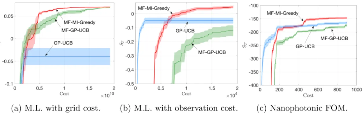
(a) M.L. with grid cost. (b) M.L. with observation cost. (c) Nanophotonic FOM.

Figure 3: Two cost settings for maximum likelihood inference task and the task of optimizing FOM for nanophotonic structures. Error bar shows one standard error over 20 runs for each experiment.

parameters are N ∈ [50,192] and G ∈ [102,106]. We follow the fidelity levels selected in

Kandasamy et al.(2017) which correspond to two lower fidelities with (N1, G1) = (97,2.15×

103), (N2, G2) = (145,4.64×104) and the target fidelity with (N3, G3) = (192,106). Costs

are defined as the product ofN and G.

Upon further investigation, we find that the grid sizes selected above for performing numerical integration do not affect the final integral values, i.e. the grid size for the lowest fidelity G1 = 2.15×103 is fine enough to compute an approximation to the integration as

using the grid size for the target fidelity. So costs taking into consideration the integration grid sizes are not an accurate characterization of the true computation costs. As a result, we propose a different cost definition that depends only on how many data points are used to compute the likelihood, i.e. the new costs for the 3 functions are (97,145,192), respectively. The results using the original cost definition are shown in Figure 3a. Note for this task we do not know the optimal likelihood, so we report the best objective value so far (simple rewards) in they-axis. Our methodMF-MI-Greedy(red) outperforms both baselines. The results using the new cost definition are shown in Figure 3b. Our method obtains a consistent high likelihood when the cost structure changes. However,MF-GP-UCB’s quality degrades significantly, which implies that it is sensitive to how the costs among fidelity levels are defined. These two set of results demonstrate the robustness of our method against costs, which is a desirable property as inaccuracy in cost estimates is inevitable in practical applications.

6.4.2 Experimental Design for Optimizing Nanophotonic Structures

The second experiment is motivated by a material science task of designing nanophotonic structures with desired color filtering property (Fleischman et al., 2017). A nanophotonic structure is characterized by the following 5 parameters: mirror height, film thickness, mirror spacing, slit width, and oxide thickness. For each parameter setting, we use a score, commonly called a figure-of-merit (FOM), to represent how well the resulting structure satisfies the desired color filtering property. By minimizing FOM, we hope to find a set of high-quality design parameters.

(13)

Traditionally, FOMs can only be computed through the actual fabrication of a structure and tests its various physical properties, which is a time-consuming process. Alternatively, simulations can be utilized to estimate what physical properties a design will have. By solving a variant of the Maxwell’s equations, we could simulate the transimission of light spectrum and compute FOM from the spectrum. We collect three fidelity level data on 5000 nanophotonic structures. What distinguishes each fidelity is the mesh size we use to solve the Maxwell’s equations. Finer meshes lead to more accurate results. Specifically, lowest fidelity uses a mesh size of 3nm×3nm, the middle fidelity 2nm×2nm and the target fidelity 1nm×1nm. The costs, simulation time, are inverse proportional to the mesh size, so we use the following costs [1, 4, 9] for our three fidelity functions.

Figure 3c shows the results of this experiment. As usual, the x-axis is the cost and

y-axis is negative FOM. After a small portion of the budget is used in initial exploration, MF-MI-Greedy (red) is able to arrive at a better final design compared with MF-GP-UCB and GP-UCB.

7. Conclusion

In this paper, we investigated the multi-fidelity Bayesian optimization problem, and pro-posed a general, principled framework for addressing the problem. We introduced a simple, intuitive notion of regret, and showed that our framework is able to lift many popular, off-the-shelf single-fidelity GP optimization algorithms to the multi-fidelity setting, while still preserving their original regret bounds. We demonstrated the performance of our proposed algorithm on several synthetic and real datasets.

8. Acknowledgments

This work was supported in part by NSF Award #1645832, Northrop Grumman, Bloomberg, and a Swiss NSF Early Mobility Postdoctoral Fellowship.

References

Alvarez, M. and Lawrence, N. D. Sparse convolved gaussian processes for multi-output regression. In Advances in neural information processing systems, pp. 57–64, 2009. 4

Bonilla, E. V., Chai, K. M., and Williams, C. Multi-task gaussian process prediction. In

Advances in neural information processing systems, pp. 153–160, 2008. 4

Boyle, P. and Frean, M. Dependent gaussian processes. In Advances in neural information processing systems, pp. 217–224, 2005. 4

Chen, Y., Javdani, S., Karbasi, A., Bagnell, J. A., Srinivasa, S., and Krause, A. Submodular surrogates for value of information. InProc. Conference on Artificial Intelligence (AAAI), January 2015. URL https://bit.ly/2QEfJnZ. 6

Contal, E., Perchet, V., and Vayatis, N. Gaussian process optimization with mutual in-formation. In International Conference on Machine Learning, pp. 253–261, 2014. URL https://bit.ly/2x7EEbw. 3,8,17

(14)

Davis, T. M., M¨ortsell, E., Sollerman, J., Becker, A. C., Blondin, S., Challis, P., Clocchiatti, A., Filippenko, A., Foley, R., Garnavich, P. M., et al. Scrutinizing exotic cosmological models using essence supernova data combined with other cosmological probes. The Astrophysical Journal, 666(2):716, 2007. 11

Fleischman, D., Sweatlock, L. A., Murakami, H., and Atwater, H. Hyper-selective plasmonic color filters. Optics Express, 25(22):27386–27395, 2017. 1,12

Forrester, A. I., S´obester, A., and Keane, A. J. Multi-fidelity optimization via surrogate modelling. In Proceedings of the royal society of london a: mathematical, physical and engineering sciences, volume 463, pp. 3251–3269. The Royal Society, 2007. URLhttps: //bit.ly/2xkMXRr. 2,4

Hennig, P. and Schuler, C. J. Entropy search for information-efficient global optimization.

Journal of Machine Learning Research, 13(Jun):1809–1837, 2012. URL https://bit. ly/2x5KMQC. 3,7

Hern´andez-Lobato, J. M., Hoffman, M. W., and Ghahramani, Z. Predictive entropy search for efficient global optimization of black-box functions. InAdvances in neural information processing systems, pp. 918–926, 2014. 3,4

Kandasamy, K., Dasarathy, G., Oliva, J. B., Schneider, J., and P´oczos, B. Gaussian process bandit optimisation with multi-fidelity evaluations. In Advances in Neural Information Processing Systems, pp. 992–1000, 2016. URL https://bit.ly/2Qngemh. 2,5,9,10,11

Kandasamy, K., Dasarathy, G., Schneider, J., and P´oczos, B. Multi-fidelity bayesian op-timisation with continuous approximations. In International Conference on Machine Learning, pp. 1799–1808, 2017. URLhttps://bit.ly/2N9KgMq. 2,5,11,12

L´azaro-Gredilla, M., Qui˜nonero-Candela, J., Rasmussen, C. E., and Figueiras-Vidal, A. R. Sparse spectrum gaussian process regression. Journal of Machine Learning Research, 11: 1865–1881, 2010. 4

Le Gratiet, L. and Garnier, J. Recursive co-kriging model for design of computer experi-ments with multiple levels of fidelity. International Journal for Uncertainty Quantifica-tion, 4(5), 2014. URL https://bit.ly/2PICVQu. 4

Marco, A., Berkenkamp, F., Hennig, P., Schoellig, A. P., Krause, A., Schaal, S., and Trimpe, S. Virtual vs. real: Trading off simulations and physical experiments in reinforcement learning with bayesian optimization. In2017 IEEE International Conference on Robotics and Automation (ICRA), pp. 1557–1563, 2017. URLhttps://bit.ly/2Oa4e62. 2,4

Nguyen, T. V. and Bonilla, E. V. Collaborative multi-output gaussian processes. In UAI, pp. 643–652, 2014. URLhttps://bit.ly/2D4BwCH. 4

Rahimi, A. and Recht, B. Random features for large-scale kernel machines. InAdvances in neural information processing systems, pp. 1177–1184, 2008. 4

Rasmussen, C. E. and Williams, C. K. I. Gaussian Processes for Machine Learning. MIT Press, 2006. URL https://bit.ly/2tYpBix. 3

(15)

Romero, P. A., Krause, A., and Arnold, F. H. Navigating the protein fitness landscape with gaussian processes. Proceedings of the National Academy of Sciences, 110(3):E193–E201, 2013. 1

Sen, R., Kandasamy, K., and Shakkottai, S. Multi-fidelity black-box optimization with hierarchical partitions. In Proceedings of the 29th International Conference on Machine Learning (ICML), 2018. URLhttps://bit.ly/2MSIsSQ. 2,5

Snelson, E. and Ghahramani, Z. Local and global sparse gaussian process approximations. In Artificial Intelligence and Statistics, pp. 524–531, 2007. 4

Snoek, J., Larochelle, H., and Adams, R. P. Practical bayesian optimization of machine learning algorithms. In Advances in neural information processing systems, pp. 2951– 2959, 2012. 3

Srinivas, N., Krause, A., Kakade, S., and Seeger, M. Gaussian process optimization in the bandit setting: No regret and experimental design. In Proc. International Conference on Machine Learning (ICML), 2010. URL https://bit.ly/2CNGPGc. 3,8,9,10,17

Teh, Y.-W., Seeger, M., and Jordan, M. Semiparametric latent factor models. In Artificial Intelligence and Statistics 10, 2005. 4

Titsias, M. Variational learning of inducing variables in sparse gaussian processes. In

Artificial Intelligence and Statistics, pp. 567–574, 2009. 4

van Gunsteren, W. F. and Berendsen, H. J. Computer simulation of molecular dynamics: Methodology, applications, and perspectives in chemistry. Angewandte Chemie Interna-tional Edition in English, 29(9):992–1023, 1990. 1

Wang, Z. and Jegelka, S. Max-value entropy search for efficient bayesian optimization.arXiv preprint arXiv:1703.01968, 2017. URLhttps://arxiv.org/pdf/1703.01968.pdf. 3,7,

8

Wang, Z., Zhou, B., and Jegelka, S. Optimization as estimation with gaussian processes in bandit settings. In Artificial Intelligence and Statistics, pp. 1022–1031, 2016. URL https://bit.ly/2OeSOhp. 3,8,17

Wilson, A. G., Knowles, D. A., and Ghahramani, Z. Gaussian process regression networks. InProceedings of the 29th International Conference on Machine Learning (ICML), 2012.

4

Zhang, Y., Hoang, T. N., Low, B. K. H., and Kankanhalli, M. Information-based multi-fidelity bayesian optimization. NIPS Workshop on Bayesian Optimization, 2017. URL https://bit.ly/2N5CdjH. 4

(16)

Appendix A. Proofs for §5

A.1 Proofs of Theorem 4

Proof [Proof of Theorem 4] Assume that MF-MI-Greedy terminates within k episodes. Let us useE(1)_{, . . . ,}_E(k) _{to denote the sequence of actions selected by}_MF-MI-Greedy_{, where}

E(j)_:=_L(j)_∪{h_{x, m}_i(j)_}_{denotes the sequence of actions selected at the}_jth_{episode. Further,}

let Λ_E(j) be the cost of thejth episode, and Λ_L(j)= Λ(_Ej)−λm the cost of lower fidelity actions of thejth episode. The budget allocated for the target fidelity iskλm= Λ−Pkj=1Λ

(j) L . By definition of the cumulative regret (Eq. (6)), we get

R(π,Λ) = Λ λm f_m∗ − k X j=1 q(L(j)_{∪ {h}_{x, m}_i(j)_}₎ = Λ λm f_m∗ −   k X j=1 *0 q(L(j)) + k X j=1 q(hx, mi(j))   = Λ λm f_m∗ − k X j=1 fm x(j) = Λ λm −k f_m∗ + k X j=1 f_m∗ −fm x(j) = f ∗ m λm · k X j=1 Λ(_Lj)+ k X j=1 f_m∗ −fm x(j) (7)

The first term on the R.H.S. of Eq. (7) represents the regret incurred from exploring the lower fidelity actions, while the second term represents the regret from the target fidelity actions (chosen bySF-GP-OPT).

According to the stopping condition of Algorithm 2 at Line 8, we know that when Explore-LFterminates at episode j, the selected low fidelity actions Lsatisfy

I y_L(j);fm y (1:j−1) E Λ(_Lj) ≥βj, wherey(1:_E j):=Sj u=1y (u)

E denotes the observations obtained up to episodej, andβj specifies the stopping condition of Explore-LF at episode j. Therefore

k X j=1 Λ(_Lj) ≤ k X j=1 I y(_Lj);fm y (1:j−1) E βj (8) (a) ≤ αΛ k X j=1 I y(_Lj);fm y (1:j−1) E =αΛγL

(17)

where step (a) is because αΛ = maxBα(B) > _β1_j for j ∈ [k]. Recall that β1 = _o₍√1_Λ₎. Therefore, f_m∗ λm · k X j=1 Λ(_Lj)≤ f ∗ m λm ·αΛγL. (9)

Note that the second term of Eq. (7) is the regret of MF-MI-Greedy on the target fidelity. Since all the target fidelity actions are selected by the subroutine SF-GP-OPT, by assump-tion, we knowPk

j=1 fm∗ −fm x(j)

=√Cγmkλm≤ √

CγmΛ. Combining this with Eq. (9) completes the proof.

A.2 Proof of Corollary 5

To show that running MF-MI-Greedy with subroutine GP-UCB (Srinivas et al.,2010), EST (Wang et al.,2016), or GP-MI(Contal et al.,2014) in the optimization phase is no-regret, it suffices to show that the candidate subroutines GP-UCB, EST, and GP-MI satisfy the assumption onSF-GP-OPT as provided in Theorem4. From the references above we know that the statement is true.