Accepted Manuscript
Title: MINLP-based Analytic Hierarchy Process to simplify multi-objective problems: application to the design of biofuels supply chains using onfield surveys
Author: J. Wheeler J.A. Caballero R. Ruiz-Femenia G. Guill´en-Gos´albez F.D. Mele
PII: S0098-1354(16)30330-1
DOI: http://dx.doi.org/doi:10.1016/j.compchemeng.2016.10.014
Reference: CACE 5585
To appear in: Computers and Chemical Engineering
Received date: 28-4-2016
Revised date: 18-10-2016
Accepted date: 24-10-2016
Please cite this article as: Wheeler, J., Caballero, JA., Ruiz-Femenia, R., Guill´en-Gos´albez, G., & Mele, F.D., MINLP-based Analytic Hierarchy Process to simplify multi-objective problems: application to the design of biofuels supply chains using on field surveys.Computers and Chemical Engineering http://dx.doi.org/10.1016/j.compchemeng.2016.10.014
This is a PDF file of an unedited manuscript that has been accepted for publication. As a service to our customers we are providing this early version of the manuscript. The manuscript will undergo copyediting, typesetting, and review of the resulting proof before it is published in itsfinal form. Please note that during the production process errors may be discovered which could affect the content, and all legal disclaimers that apply to the journal pertain.
MINLP-based Analytic Hierarchy Process to simplify
multi-objective problems: application to the design of biofuels supply
chains using on field surveys
Wheeler, J.; Caballero, J. A.; Ruiz-Femenia, R.; Guillén-Gosálbez, G.*; Mele, F. D.
Reader in Process Systems Engineering
Centre for Process Systems Engineering
Imperial College of Science, Technology and Medicine
Phone number: +44 (0)20 7594 1478
Roderic Hill Building, C612
London SW7 2BY, United Kingdom
*Corresponding author
Highlights
We calculate weighting factors on the basis of the Analytical Hierarchy Process.
Weights reflect experts’ preferences on a given problem with maximum consistency.
We use a weighting-based approach to solve multi-objective optimization problems.
The proposed framework is applied to the sugar cane industry in Argentina.
Abstract
Multi-objective optimization (MOO) is at present widely used in engineering systems design and planning. The solution of such a problem leads to a set of efficient solutions (Pareto set) from which decision-makers should identify the one that best fits their preferences. Generating this set requires large computational efforts, and the post-optimal analysis of the solutions becomes difficult as the number of objectives increases. This work introduces an approach based on the Analytic Hierarchy Process (AHP) to overcome these limitations. Through the definition of an aggregated objective function, a single-objective model is constructed that provides a unique Pareto solution of the original MOO model. The AHP is combined with a mixed-integer non-linear programming (MINLP) formulation that simplifies its application and is particularly suited to deal with many objectives (e.g. sustainable engineering problems). The capabilities of the approach are demonstrated through a case study addressing the sustainable sugar/ethanol supply chain design
problem.
Keywords: optimization; sustainability; multi-criteria decision-making; weighting.
1 Introduction
Multi-objective problems are found in many fields, such as production, services and entertainment. The wide variety of conflicting interests that emerge in engineering systems, such us economic, environmental and social concerns, has led to a large set of MOO problems (Grossmann and Guillén-Gosálbez, 2010). In the recent past, MOO has been extensively used in sustainable engineering problems in which economic, environmental and social criteria must be accounted for in the analysis (Guillén-Gosálbez and Grossmann, 2009; Yue et al., 2014; Miret et al., 2016). For example, Kostin et al. (2012) introduced a stochastic MOO model that optimizes profit and financial risk, whereas Kravanja and Čuček (2013) developed a model to explore the trade-off between profit and sustainability indexes. García and You (2015) contrast capital and operating expenditures with environmental impacts. Some works have applied as well MOO in the area of energy systems optimization (Guillén-Gosálbez et al., 2009; Gebreslassie et al., 2012; Antipova et al., 2013).
Different approaches, known as multi-criteria decision-making (MCDM) techniques (Marler and Arora, 2004), can be found in the literature to tackle multi-objective problems involving conflicting criteria. These MCDM strategies are roughly classified into two groups: multi-objective decision-making methods, usually referred to as multi-objective optimization (MOO), and multi-attribute decision-making methods (Cortés-Borda et al., 2013, Geldermann and Rentz, 2005). The former group identifies optimal solutions from a set of feasible points (Pareto solutions) using search methods limited by constraints of different nature, while the latter group evaluates and selects alternatives departing from a set of them and based on defined attributes.
MOO models, whether linear, nonlinear or mixed-integer, typically contain an infinite number of Pareto optimal solutions. These Pareto points represent compromise situations, in the sense that it is impossible to enhance one criterion without worsening any of the others. Calculating the complete set of Pareto points of an MOO model may be computationally challenging, as it requires intensive information processing and storage capacity. These limitations could be circumvented by selecting a subset of Pareto solutions that are particularly appealing and which should be passed to the decision-maker for identifying the final one to be implemented.
A number of works have addressed the problem of reducing the size of the Pareto set of an MOO problem. One possible manner to accomplish this is to incorporate the user’s preferences in the resolution process in order to dive into a special region of the Pareto set. This is the underlying idea followed in the works by Branke et al. (2001, 2004), in which evolutionary algorithms are employed. Messac et al. (2003) introduced the normal constraint method to limit the size of the Pareto set, while Matusiewicz and Osyczka (2003) use decomposition strategies for the same purpose. For problems with convex Pareto optimal fronts, Deb (2003) presents a modified domination criterion to reduce the computational burden of the model. To reduce potential disturbances when producing the Pareto front, Deb and Gupta (2005) present some approaches with enhanced robustness. Farina and Amato (2004) introduce a dominance concept derived from fuzzy optimality to narrow down the Pareto set. More recently, Antipova et al. (2015) applied Pareto filters to reduce the Pareto set and facilitate the post-optimal analysis of its solutions.
In this work, we explore the combined use of AHP and MOO when addressing the solution of complex MOO models. We propose to solve, instead of the original MOO problem, an auxiliary single-objective optimization (SOO) problem that optimizes an aggregated objective function constructed using weights calculated by the Analytic Hierarchy Process (AHP) (Saaty, 1980). The AHP translates qualitative judgments (elicited from a set of surveys completed by “experts” in the
problem) into quantitative information. Note that there are many other methods for obtaining weighting factors, e.g. SMART (Simple Multi-Attribute Rating Technique) (Edwards, 1977) and SWING (Von Winterfeldt and Edwards, 1986). However, among them the AHP is one of the most widely used in academic and also in industry (Vaidya and Kumar 2006), which has motivated its choice in our work.
Unfortunately, the application of the AHP process poses some challenges. First, the need of gathering different opinions in the AHP surveys so as to reflect a wider spectrum of preferences can sometimes lead to inconsistencies and meaningless weighting factors (Pöyhönen and Hämäläinen, 2001). In addition, the complexity of the AHP method grows with the number of criteria, as this approach is based on performing pairwise comparisons between objectives. We present here an MINLP-based AHP that overcomes these limitations by automatically generating weights with maximum consistency from preferences expressed in a very simplified manner. The customized MINLP greatly facilitates the AHP application by reducing the amount of information required from decision-makers while ensuring that their preferences are expressed in a consistent manner. The MINLP-based AHP can be used to simplify MOO problems, as we do here, or as a standalone tool to facilitate the AHP application anywhere else. The capabilities of our approach are illustrated through its application to the design of biofuels supply chains.
The article is presented in the following order. The next section describes the mathematical background underpinning the approach presented, followed by the description of the proposed methodology itself. Then, we present a case study (already validated and tested in previous works) that is based on an Argentine sugar cane supply chain (SC). Next, we present some numerical results and discuss them. In the last section of the paper, the conclusions are drawn.
2 Mathematical background
2.1 Multi-objective optimization
A formal representation of a typical MOO problem is given by P1.
01 0 0 , , min 1 , , y x g(x,y) h(x,y) t. s. (x,y) f (x,y) f .., (x,y),. f k K (P1)In P1, fk(x,y) represents the k-th (k = 1,… K) objective function; h and g stand for the equality and
inequality constraints that the solution sought should satisfy, respectively; and x and y are the continuous and binary variables of the problem, respectively.
We propose to solve this problem P1 by using an auxiliary single-objective model. To this end, we create an aggregated objective function (a composite function of the individual objectives) calculated as a linear weighted sum of individual terms (i.e. objectives) whose weighting factors are obtained using an enhanced AHP methodology. Thereby, we build a SOO model with the same equality and inequality constraints as in P1, but with a single-objective (scalar) objective function rather than a multi-objective (multi-dimensional) one. Thus, this auxiliary single-objective model will provide a single Pareto point of P1, thereby avoiding the exhaustive exploration of its Pareto set and consequently simplifying the entire analysis.
The key issue in this reformulation is the way in which the weighting factors are chosen. We use the AHP method combined with an optimization model to calculate the weighting factors. This optimization model calculates weighting factors that express the decision-makers’ preferences with
maximum consistency. Thus, P2 is formulated from P1 as follows:
01 0 0 min 1 1 , , y x g(x,y) h(x,y) t. s. (x,y) f w .. . (x,y) f w (x,y) f w k k K K (P2)In P2, wk is the k-th weighting factor assigned to objective k. Therefore, P2 produces a unique
solution (rather than a Pareto set) that best reflects the decision-makers’ preferences. As will be later discussed in more detail, this model requires the objectives to be normalized so that they can be optimized all together.
2.2 The Analytic Hierarchy Process
The AHP (Saaty, 1980) is a multi-attribute decision-making method that supports multi-criteria problems by taking into account a hierarchy in the criteria. This method was applied to a variety of industrial problems, such as facility location (Dogan and Bahadir, 2014), supplier selection (Ramanathan, 2007) and SC redesign (Palma-Mendoza, 2014). Particularly, it was successfully implemented in cases where environmental criteria were considered together with other industrial goals, such as materials purchasing (Gloria et al., 2007) or technology selection (Meng et al., 2010). Unlike the present work, the abovementioned ones use AHP as a standalone tool (without integrating it with an optimization technique as we do here).
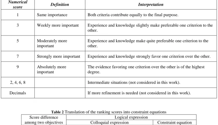
The starting point of the AHP method includes a set of surveys answered by N decision-makers. These decision-makers –academics, technicians or business people–, are asked to define a hierarchy of criteria (i.e. objectives), from the most to the least important. Next, the traditional AHP process asks the respondents to perform pairwise comparisons between the K objectives. These comparisons make use of the standard Saaty scale, which goes from 1 to 9 (Table 1). Note that even values, 2 to 8, would here reflect intermediate situations. Moreover, rational numbers can also be used if more refinement is required.
Next, N “coefficient matrices” are built using these comparisons values. Let An be a coefficient
matrix associated with a respondent n (n = 1,…, N). An contains the relative importance between the
K different objectives. The elements of An will be denoted by anij, where n is an identifier of the
survey respondent. Subscripts i and j represent the element position (row and column, respectively). Since i = 1,…, K, and j = 1,…, K, then K K
n
A . Therefore, a Saaty coefficient matrix An is
constructed by filling its upper triangle with the pairwise comparison factors:
nKK nK K n n a a a a .. : : .. 1 1 11
The element anij is the Saaty scale value resulting from the comparison between objectives i and j
made by stakeholder n. Then, it holds that anji =1/ anij and the diagonal elements anii =1
(self-comparison).
Stakeholders may have different backgrounds, knowledge and interests, so they will very likely produce matrices whose values differ to a certain extent. This creates the need to harmonize such matrices in a valid way. Moreover, according to the general AHP method, prior to the matrices aggregation, it is necessary to check the consistency of each of them. Matrix consistency stands for the logical quality of the responses given by a person who performs a survey (see next subsection). Let λmax be the maximum eigenvalue of a given matrix An, then, a consistency index (CI) is
calculated for each matrix (Eq. 1) as follows. ) 1 ( ) ( max K K CI (1)
When λmax of An is K, then CI = 0, which means that the Saaty matrix is fully consistent. If λmax of
An is greater than K, then CI will also be greater than 0. To determine whether the value of CI is
acceptable or not, a threshold value is used, RI, which is a random consistency index defined by Saaty (1980) and available in tables for matrices of different sizes. A consistency ratio CR is then calculated as in Eq. 2.
RI CI
CR (2)
If CR is equal or lower than 0.1 (90% of consistency in the comparisons, and 10% of inconsistency) then matrix An is accepted, otherwise is dismissed (Saaty, 1990). Hence, the smaller the CR value,
the better. Hence, smaller CR values imply better consistency, and from Eq. (1) it is clear that this can be accomplished by minimizing the value of λmax, which is always greater or equal than the
dimension of the matrix K.
After checking the consistency of every individual coefficient matrix An, we can follow two basic
methods to aggregate the respondents’ preferences. The choice of a particular method depends on whether we consider the group of stakeholders behaving as a single decision-maker or as disjoint individuals (Aczel and Saaty, 1983; Forman and Peniwati, 1998; Escobar and Moreno-Jimenez, 2007). For the former case (which is the one followed in this work due to the nature of the matrices), we aggregate individual judgments (AIJ) by using the element-by-element geometric mean calculated over all of the individual matrices. In the latter, the geometric mean should be instead calculated over the priorities (eigenvectors) resulting from these matrices (aggregation of individual priorities, AIP).
The next step in the AHP process, following the AIJ aggregation method, is to construct a new matrix M using the consistent matrices An, in which, as said before, each element mij is the
element-by-element geometric mean of the elements of each An (Eq. 3).
K K M , N N n nij ij a m 1 1
(3)Finally, the weights are obtained from matrix M by calculating the normalized maximum eigenvalue (Saaty, 1990) (Eq. 4).
K i w w m i K j j ij max 0 1, , 1
(4)where wj are the components of the normalized eigenvector, i.e. the weights sought.
2.3 Consistency in the AHP
A matrix is deemed consistent if its elements satisfy transitivity and reciprocity assumptions. Transitivity implies that aij = aik·akj. For example, let us consider a decision-maker for whom
objective one is two times more important than objective two (a1,2 = 2), and objective two is three times better than objective three (a2,3 = 3). If objective one is six times better than objective three, then transitivity holds. Reciprocity means that aij = 1/aji. For instance, if a decision-maker prefers
objective one twice as much as objective two (a1,2 = 2); therefore, objective two should be half preferable than objective one (a2,1 = ½). The consistency index (CI) and consistency ratio (CR) defined by Saaty (1980) aim at guaranteeing a necessary degree of compliance with the aforementioned properties. A deep discussion about the acceptance or rejection of AHP matrices can be found elsewhere (Alonso and Lamata, 2006). Note that the scale employed to represent decision-makers’ judgements lies at the core of this discussion, as when K increases the level of consistency may fall outside acceptance limits (Murphy, 1993)
The number of comparisons (NC) required to build the Saaty matrix increases with the number of objectives according to Eq. 5. Therefore, the comparison process may become cumbersome for the respondent, making it more difficult to reach good consistency levels in the AHP matrices.
) ( 2 1 2 k k NC (5)
In order to avoid consistency problems and simultaneously reduce the time spent on answering the surveys, we propose an MINLP that automatically generates consistent weights from a ranking of objectives. Hence, our algorithm generates, from a simplified survey based on a customized scale and in a fast and robust manner, a coefficient matrix that minimizes the CI. This approach prevents respondents from providing inconsistent weights, thereby facilitating the decision-making process.
3 Proposed methodology
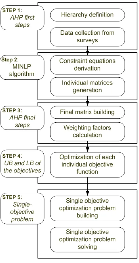
Our approach comprises five steps described in detail in the ensuing sections (see Fig. 1).
Step 1: AHP hierarchy definition and data collection
Following the AHP method, a decision hierarchy is first constructed, where the overall objective is on the top, while the individual ones are arranged in branches downwards. A number of surveys are collected from the decision-makers (respondents), who are asked to evaluate the objectives according to their preferences. In the evaluation process, an arbitrary scale can be used, for example, from 0 to 10 (where 10 represents the score for the most important objective/criterion). As a result of this step, a ranking of objectives is obtained, from more to less important.
Step 2: Generation of pairwise matrices from simplified preferences by using an MINLP algorithm for each individual set of preferences
In this step, the individual pairwise coefficients of the comparison matrices (corresponding to each respondent) of the AHP methodology are obtained using an optimization algorithm. The objective of the algorithm is to determine the elements of matrix An (based on the Saaty scale) that minimize
the maximum eigenvalue (λmax) (i.e. that maximize the consistency level). Given that equation 4 has a bilinear term, the model is non-linear and non-convex. Therefore, the resulting formulation leads to a non-convex MINLP. The detailed MINLP formulation is described in detail next.
Objective function:
The MINLP model seeks to minimize the consistency index (recall that lower CI values imply better consistency). This is equivalent to minimizing the maximum eigenvalue λmax (Eq. 4):
max
Constraints:
To compute the maximum eigenvalue, we first need to build the pairwise comparison matrix. Rather than providing the coefficients of the matrix ourselves, we define a set of binary variables that will automatically identify the best coefficients so as to optimize the consistency index. Obviously, we cannot let the model decide arbitrarily those values, as the weights obtained in this manner would barely reflect the decision-makers’ preferences. Hence, additional constraints are required to ensure that the values of the binary variables are consistent with the decision-makers’ preferences. These preferences are expressed as a ranking of objectives rather than through pairwise coefficients, thereby simplifying the AHP application.
Hence, we start by forcing each element of the upper triangle of the coefficient matrix to take a unique value of the Saaty scale (Eq. 7 and Eq. 8).
j i y q a s ijs s ij
(7) j i y s ijs
1 (8)where qsare the Saaty parameters (1, 3, 5, 7, 9) and yijs is a binary variable that is one if the Saaty
value s (qs ) is assigned to the comparison between i and j, and it is zero otherwise. Hence, Eq. 7
defines the pairwise comparison coefficients from these binary variables, while Eq. 8 ensures that for every comparison between i and j, a single value of the Saaty scale is selected.
The elements of the lower triangle can be calculated according to Eq. 9.
j
i
a
a
ij ji,
1
(9)This condition can be enforced using the following constraint together with Eq. 7 (note that this reformulation is linear and therefore more convenient):
j
i
q
y
a
s s ijs ji
1
(10)The normalized eigenvector elements wi required to compute the consistency index (Eq. 11) lie
between zero and one (Eq. 12) and sum up one (Eq. 13):
i w w y q w w a i K j j s ijs s i K j j ij
, 0 max 1 max 1 (11) i wi 1, 0 (12) 1
i i w (13)The minimum value of λmax is equal to the number of objectives (i.e. dimension of the square matrix, K) (Eq. 14).
K
max
Equation 11 includes a product of a binary variable times a continuous one (yijs ·wj). This term can be linearized as follows: i w yw q i K j s ijs s
, 0 max 1 (15)
s ijs ijs U y i j s U q yw , , , max 0 (16) s j i y U w yw y Uwj (1 ijs) ijs j (1 ijs) , , (17) Where ywijs is now an aggregated auxiliary variable defined via constraints 16 and 17.
Additional constraints are derived based on the ranking of objectives provided by decision-makers. To this end, we define a number of potential relations between objectives based on the Saaty scale (Table 1). Using the numerical difference between the rankings of two consecutive objectives, it is possible to establish logical expressions of relative importance between criteria (Table 2). These logical relationships are then included as constraints in the MINLP. Following this approach, decision-makers define K-1 comparisons between objectives, which are then converted into algebraic constraints of the MINLP model. Let us note that it would be possible to define relations between more than two objectives, but this would lead to more formulations and also to the need to devise and fill in more complex surveys.
For every survey, we solve the MINLP to find the matrix with maximum consistency according to the preferences established in that survey. Hence, the MINLP provides as output the pairwise comparison coefficients as well as the weights assigned to every objective according to a given preference elicited in a specific survey. The MINLP can be expressed in compact form as follows:
min max s. t. Eq. 7-8, 10, and 12-17 K-1 ranking constraints w , w
0,1Step 3: Computation of weights for the individual objectives from the outcomes of the MINLP
In this step, we aggregate the matrices calculated for each survey n. These matrices are filled using the above described algorithm, that is, based on the decision-makers’ comparisons. Hence, it makes little sense to get the priorities of each matrix (eigenvectors) separately. Therefore, the weights for each branch of the hierarchy are obtained by applying the Aggregation of Individual Judgements (AIJ) method. This approach first merges the individual matrices, and then calculates the weights (eigenvectors) from the aggregated matrix. Hence, in the AIJ approach, the individual priorities of the respondents are of little interest (the respondents do not give their opinion on all the branches of the hierarchy tree).
Following this approach, we compute the element-by-element geometric mean to get the final matrix M (Eq. 3). Finally, we use M to obtain the weighting factors (wk) needed to solve the SOO
problem (Eq.4).
Step 4: Reformulation of the MOO into an SOO: Normalization step
Each of the objectives needs to be normalized before being summed and weighted in the aggregated objective function. To this end, each objective in P1 is first optimized separately. Let (xk,yk) be the
bounds on each objective function k ( fk and fk , respectively) are calculated as follows:
( , ),..., ( , )
max ) , ( ),..., , ( min 1 1 1 1 K K k k k K K k k k y x f y x f f y x f y x f f Once the bounds are obtained, we normalize the objectives as follows:
) , ( ) , ( ) , ( ) , ( ˆ y x f y x f y x f y x f f k k k k k (18)
Where fˆkis the normalized value for objective k. Step 5: Construction and solution of the SOO model
The lower and upper bounds on the objectives (previous step) and the weights obtained in step 3 are utilized to construct an aggregated objective function for the reformulated problem P3 as follows:
01 0 0 ) , ( ˆ min 1 , , y x g(x,y) h(x,y) t. s. y x f p k k k
(P3)The solution of this SOO problem (P3) will provide the best Pareto solution according to the decision-makers’ preferences.
Remarks:
- The solution of P3 is guaranteed to be a Pareto optimal point of P1 because model P3 represents a single iteration of the weighted sum method applied to P1. See Ehrgott (2005) for more details. - The normalization procedure described above ensures that all of the objective function values belong to the interval [0, 1]. Note, however, that any other normalization method could be applied for the same purpose (Cloquell et al., 2001).
- The MINLP contains bilinear terms (Eq 10), which may lead to the existence of multiple local optima (i.e. multimodality). Hence, a global optimization package should be used to ensure convergence to the global optimum within a given epsilon tolerance.
- Other MCDM methods can be applied to obtain the weighting factors to be appended to the objectives, such as ranking methods (Yoon and Hwang, 1995), categorization methods, rating methods and pairwise comparison methods (Marler and Arora, 2004).
- The same approach presented in step 2 for generating matrices with maximum consistency can be used, with little modification, to increase the consistency of a given coefficient matrix S with elements sij. To this end, we would solve an MINLP which would seek to minimize the distance
(quantified via norm 1 or norm 2) between the new weights and the current ones subject to an additional constraint that enforces the eigenvalue to be below a given upper bound ensuring a minimum consistency level (Eq. 19).
i j ij ij s a min , (19)the formulation would include the constraints given by Eq. 7, 8, 10 and 12 to Eq. 17.
4 Case study
We test the capabilities of our approach through its application to the model presented by Mele et al. (2011), who first addressed the problem of designing a sugar/ethanol SC considering economic and environmental issues simultaneously. This problem was later studied by Kostin et al. (2011) and Copado-Méndez et al. (2013).
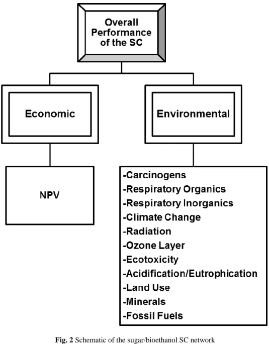
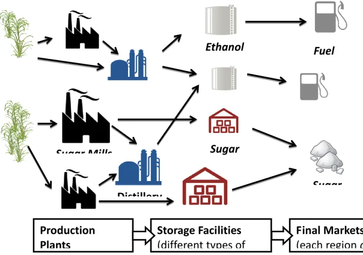
Fig.2 depicts the three-echelon SC network considered for the analysis. It encompasses a number of production plants (supplied by sugar cane growers), storage facilities, and markets with an associated demand for each of the final products: white sugar, raw sugar and fuel grade ethanol. The SC operates over a time horizon divided into annual periods, and considering a geographical area split into regions that match the 24 provinces of the country. Each region has an associated sugar cane production capacity per period.
According to the production technology, five types of production facilities can be established at each region. Raw and white sugar can be produced either by technologies T1 or T2, whereas ethanol can be obtained through technologies T3, T4 and T5. Byproducts of T1 and T2, molasses and honey, respectively, are converted through T3 and T4 into ethanol, while T5 produces ethanol directly from sugar cane. After being stored in appropriate facilities, products are sent to the customers (markets): technology S1 is used for solid products and S2 for liquids. Several emissions and wastes generated by the process activities are considered in the analysis. Regarding transportation, heavy trucks carry sugar cane, lorry trucks transport sugar and tank trucks transport ethanol, all of them using transportation links that can be established between any SC nodes.
Given are a number of parameters such as: time horizon, product prices, cost data for production, storage and transportation, demand forecast, tax and interest rates, capacity data (for plants, warehouses and transportation means), capital investment, landfill tax, and environmental data (emissions and raw material consumption linked to the SC activities). The aim of the SC design problem is to find the SC network topology of the sugar/bioethanol SC and the strategic decisions to be made so as to minimize the environmental impacts while maximizing the economic benefit simultaneously. The environmental impact values are assessed through an LCA (Life Cycle Assessment) analysis. In other words, it is necessary to decide, for each region and time period: (i) the type and number of production and storage facilities to be installed or expanded; (ii) the links between facilities and the required transportation means; and (iii) the production rates and material flows (raw material, wastes and final products). Data considered for this analysis can be found in Appendix A.
Mele et al. (2011) solved the aforementioned problem by formulating an MOO mixed-integer linear programming (MILP) formulation. The interested reader can find details on this MILP model in the original publication. The model optimizes, at the same time, the economic profit, quantified via the net present value (NPV), and the environmental performance, assessed through a set of LCA-based metrics, in a similar way as was done in previous works by the authors (Mele et al. 2005; Guillén-Gosálbez et al., 2009). Note that the AHP has been used in the LCA literature as a weighting method to weight impact categories in the Impact Assessment phase of an LCA study (Finnveden 1999), and it has been shown to improve LCA studies (Miettinen and Hämäläinen, 1997; Pineda-Henson and Culaba, 2004). AHP has also been combined with LCA-based environmental performance indicators to address environmental assessment (Hermann et al., 2007), but to our best
knowledge, never integrated with mathematical programming.
Hence, the MOO problem has the following 12 objectives: (a) NPV as the economic indicator; and (b) 11 environmental impact categories taken from the Eco-indicator 99 methodology (Appendix B), which include: (1) Carcinogens, (2) Respiratory organics, (3) Respiratory inorganics, (4) Climate change, (5) Radiation, (6) Ozone layer, (7) Ecotoxicity, (8) Acidification/eutrophication, (9) Land use, (10) Minerals, and (11) Fossil fuels.
The environmental methodology used, Eco-indicator 99, groups the impacts into three damage categories: 1 to 6 are aggregated into Damage to Human Health (HH), categories 7 to 9 belong to Damage to Ecosystem Quality (EQ), and categories 10 and 11 belong to Damage to Resources (RS). Furthermore, Eco-indicator 99 provides weighting factors for each of these damage categories. The weighting factors are derived from a panel of experts, and the particular values vary according to the “perspective” considered by the panel: hierarchist, individualist or egalitarian. Note that one could use these weighting factors to reformulate the MOO model into an SOO one (or bi-objective, if the NPV is also considered). This approach, however, would produce a solution that would reflect the Eco-indicator 99 panel of experts’ preferences, which are too general and therefore not tailored to any specific environmental problem. Hence, a more effective approach to tackle the problem is to elicit the experts’ preferences regarding the SC design problem itself. These regional experts have deeper understanding of the problem and consequently can take better decisions. As an example of the potential limitations of using general weights, note that the geographic scope of a given impact is barely covered in any LCA, despite being of utmost importance for the Argentinean stakeholders. Therefore, using general weights established by panel of experts may lead to poor and meaningless solutions that neglect the context of the environmental problem.
5 Application to the case study
Each of the steps of our approach is described next in the context of the ethanol SC design problem. Step 1:
Fig. 3 shows the hierarchy tree constructed with the objectives of the SC design problem. To obtain the weighting factors for the SOO model, two groups of 10 experts each were asked to rank the objectives within the same hierarchy level. The first group, composed of PhD students with substantial exposure to LCA and SC design research, performed the evaluations for the objectives in the environmental branch. The second group, conformed by engineers from the local sugar/ethanol industrial activity, compared economic and environmental indicators bearing the enterprise goals in mind.
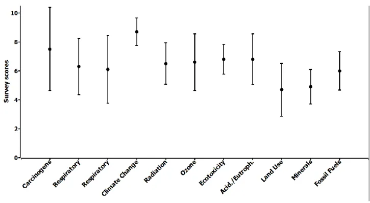
Experts answered the surveys individually without having the chance of reaching any consensus among them. In the environmental impact surveys, they were asked to appraise the importance of the 11 impacts in a 0-10 scale (in order to avoid consistency degradation). The objectives in each survey were sorted from most to least important. On the upper level of the hierarchy tree, where only economic and environmental issues are compared, the expert was asked to make one single comparison between both criteria using the Saaty scale. Fig. 4 shows the average and standard deviation of the experts’ valuations of the impacts in a 0-10 scale.
Fig. 4 shows that experts consider carcinogens and climate change (HH) as the most important impacts, while land use and minerals (RS) are the least important. The other objectives are virtually valued in a similar way. Cancer is perceived as a very serious disease, with many people suffering
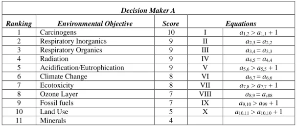
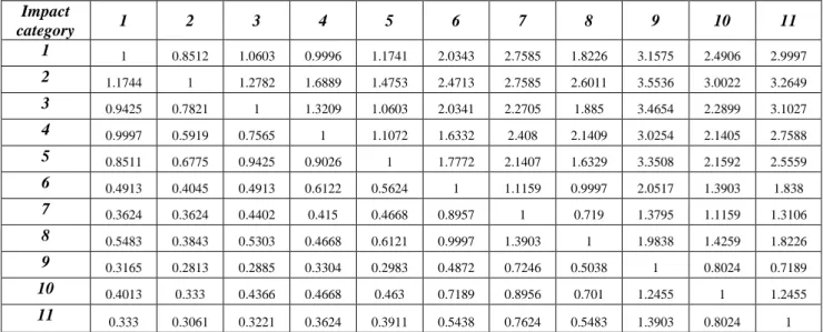
its consequences either directly or indirectly. Meanwhile climate change is one of the main challenges faced by society and constantly being discussed in the media. Hence, it is not surprising that both categories are given more importance than the others. The low standard deviation of climate change (Fig. 4) is quite remarkable and evidences the global awareness on this topic. Conversely, the lower rated impacts are less known and the general social concern on them is still budding. Note that the respondents come from the same geographic region, so they may have similar preferences. Table 3 shows the scores assigned by decision-makers to each impact category.
Step 2:
The ranking values given by decision-makers (A to J in Table 3) were used to define 10 constraints that were added to the MINLP. First, for each respondent, the 11 objectives were ranked according to their score from the most important to the least important. The constraints shown in Table 4 were then derived based on these scores for respondent A. The resulting mathematical formulation was implemented in GAMS® v.24.0.2 and solved with the general-purpose MINLP solver BARON, which guarantees convergence to the global optimum within an epsilon tolerance. The problems were solved in an Intel® Core 2 Duo, 4Gb RAM computer. Each model includes 464 single variables, 319 discrete variables and 266 constraints, and leads to a CPU time of around 30 min for an optimality gap of 0%. Let us note that the processing time required by the analyst to translate each survey into model equations is about 15 minutes. We obtain therefore 10 Saaty matrices with the maximum possible consistency for each respondent’s preferences.
Step 3:
After obtaining the 10 individual coefficient matrices for the environmental criteria, we calculated a harmonized matrix according to Eq. 3 (see Table 5). For the upper level in the hierarchy tree, a single comparison matrix was obtained in a similar way by computing the geometric mean of the individual comparisons (made in step 1) between economic and environmental concerns. This last matrix is shown in Table 6.
For both matrices (Table 5 and Table 6), we obtained the corresponding weights (eigenvectors) assigned to each objective. Table 7 displays the weights (ωb) for each environmental impact b. For
comparison purposes, the Eco-indicator 99 priorities (under the three perspectives) are listed as well in the same table. Table 8 shows the weighting factors for the environmental (ωenv) and economic
(ωNPV) indicators, whereas Table 9 shows the combined weights (after merging all the weights) for
the 12 criteria considered in this study. The combined environmental weights were calculated as in Eq. 20. k k env b k , / is an environmental objective, (20)
whereas the economic weight ωNPV, is the same in all of the cases, as it does not depend on the
individual weights assigned to each environmental indicator. Table 9 also shows the Euclidean distance between the AHP weighting factors and those taken from the Eco-indicator 99. These results reinforce the observation made when analyzing Fig. 4, namely, that the weights given by a panel of general experts may differ greatly from the weights established by those regional experts specialized on the specific problem.
Step 4:
The MILP-SOO models that optimize each individual objective separately were implemented in GAMS (Rosenthal, 2015) and solved with CPLEX 11.0 on a PC with AMD Phenom(tm) II N830 Triple-Core processor (4Gb RAM). Each model includes 47,249 single variables, 10,962 discrete variables and 48,546 constraints, with the associated CPU time ranging from 4.1 to 18.2 seconds.
Table 10 shows the solutions found, whereas Table 11 shows the extreme values obtained for each objective function.
Step 5:
Model P3 was constructed and solved using the weights obtained in step 3. The model size is similar to that of the SOO models in step 4. A solution with an absolute optimality gap of 10-4 was obtained in 551 seconds using the same processor as in step 4.
6 Results and discussion
The SOO problem (P3) was solved first using the AHP weights, and then using the weighting factors given by the three Eco-indicator 99 perspectives (Table 9). Finding these solutions took 359, 314 and 404 seconds for the hierarchist, individualist and egalitarian perspectives, respectively, for an optimality gap of 10-4, with the same piece of equipment as before. Table 12 shows the corresponding objective function values. Essentially, the egalitarian solution differs greatly from the AHP-based one in terms of NPV value (44%), and less (11%) in terms of environmental impacts. On average, the largest mismatch corresponds to minerals, and the most similar impacts values correspond to respiratory diseases by organics and climate change. The AHP solutions attempts to reduce climate change more than the other solutions, incurring in an extra cost that makes the NPV drop compared to the maximum NPV solution.
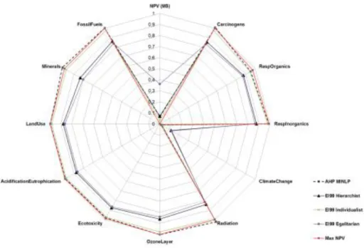
A radar chart (Fig. 5) is plotted to show the normalized value reached by every SOO solution in each criterion. The normalization procedure is that explained in step 4. Every line in Fig. 5 stands for a solution that links its performance in every criterion (objective function). The dashed line with starred markers is the solution resulting from the SOO problem using the AHP-based weights. The line with squared markers is the extreme solution of the MOO problem with maximum NPV. The solutions corresponding to the SOO problem with the Eco-indicator 99 weighting are depicted by triangles (hierarchist), diagonal crosses (individualist) and diamonds (egalitarian). As observed, some objectives are strongly correlated, as when one increases so do the others and vice versa (acidification/eutrophication correlates with ecotoxicity, while respiratory inorganics correlates with respiratory organics). The p-value test for the hypothesis of no correlation has been used to justify this observation in a quantitative way. All p-values fall below a significance level of 0.05; hence the correlation among the k objectives is significant.
A further analysis shows that the AHP, hierarchist and individualist solutions feature high NPV values (low values indeed after normalizing the original NPV values). The last row of Table 12 shows the Euclidean distance of the solutions to the maximum NPV solution. According to these figures, the individualist solution is the closest one to the maximum NPV one, whereas the egalitarian solution is the farthest one. The AHP-based solution is relatively close to the maximum NPV one, mainly because they both show similar environmental impacts despite differing in NPV values.
Three specific solutions for the sugar/ethanol SC design problem are chosen for comparison purposes: the solution with maximum NPV, the one obtained by applying the proposed AHP-based method and one of the solutions coming from the Eco-indicator 99-based weighting factors (hierarchist perspective). This perspective is used more often by analysts than the egalitarian or
individualist ones.
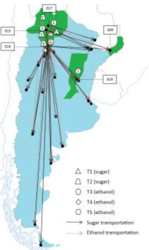
Fig. 6 shows the SC structure corresponding to each solution, specifying the number and type of production facilities, their location and the existence of distribution channels. Due to space limitations, we show only the decisions associated with the first year of the 6-year time horizon of the model. Storage facilities are not represented for clarity.
The solution with maximum NPV has the lowest number of installed facilities (9 in total). This design entails the lowest possible costs to satisfy the SC demand. Here, technologies T2 and T4 (production of sugar and ethanol from honey) prevail. Conversely, the AHP solution leads to the highest number of installed facilities (13 facilities of different types: T1, T2, T4 and T5). In this case study, the Eco-indicator 99 solution represents an intermediate situation (12 facilities) that gets closer to the AHP solution compared to the maximum NPV one. In all three solutions, transportation needs are rather similar and therefore not presented.
The maximum NPV and AHP-based solutions show relatively close capital investments: 1,827.4 and 2,022.2 M$, respectively. The distribution network shows no big differences, since in all of the cases the demand requirements need to be met. The hierarchist solution presents higher plant investment (3000 M$) than the AHP-based one. This illustrates the different results that can be generated when decisions are made on the basis of general panels of experts (Eco-indicator 99) in lieu of local stakeholders. In this particular case, SC configurations are similar indeed, mainly because the weightings factors presented in Table 9 are also similar. On the other hand, the environmental effects look rather diluted, since the NPV is highly rated among the various objectives.
7 Conclusions
This paper presents a methodology to solve MOO problems that integrates mathematical programming with the AHP, a widely used and well established multi-attribute decision-making algorithm. In essence, our approach identifies a single Pareto point that is consistent with the decision-makers’ preferences, thereby simplifying greatly the analysis. A real-world case study based on the sugar/ethanol industry in Argentina was used to demonstrate the capabilities of the proposed methodology.
Numerical results allow us to draw some important conclusions. First, the weighting factors derived from the proposed AHP-based methodology (which are consistent with the preferences of a set of decision-makers with deep knowledge on the problem) may differ significantly from the weighting scheme used in general methodologies, such as the Eco-indicator 99. Hence, using general approaches in a particular problem might lead to solutions that do not fully reflect the stakeholders’ preferences. Second, the complexity of MOO is greatly reduced by our method: (i) the surveys can be completed more easily compared to the standalone application of the AHP; and (ii) the MOO is solved using an auxiliary single-objective model, thereby avoiding the need to calculate a large number of Pareto points.
The proposed methodology brings a new insight into the design problem by introducing consistent judgments based on the relative importance of the objectives considered. This solution provides an aggregated and comprehensive performance indicator for the entire SC. This aggregated indicator is constructed on the basis of the decision-makers’ preferences, which are explicitly incorporated in the optimization model. Our tool could assist authorities in the analysis of strategic policies in the field of agro-industries and energy, facilitating the consensus among all the players involved in the decision-making process.
Acknowledgements
The authors wish to acknowledge support from the CONICET, Argentina (project PIP 00785 and doctoral scholarship), and the Spanish Government (ENE2015-64117-C5-3-R, CTQ2016-77968-C3).
Appendix A. CASE STUDY DATA
The demands of the Argentine regions considered in the analysis are presented in Table A.1. Sugar, raw sugar and ethanol prices (537, 375 and 869 $/t, respectively) are considered constant along the time horizon as well as their respective demands in each region. The distance between two regions was calculated as the remoteness among the respective province capitals through main roads. Distance data is shown in Table A.2. The time horizon considered in our case is 6 years long. Each province of Argentina has an associated crop capacity for sugar cane that we assume constant along the time horizon. Specifically sugar cane can be grown only in 5 provinces of Argentina. The crop capacities for these regions are shown in Table A.3. The production capacities for the technologies considered in this case study are exposed in Table A.4. We consider a minimum storage capacity for solid and liquid materials of 200 tons, and a maximum capacity of 2 billion tons. We assume a storage period of 10 days. The maximum possible capital investment has been set to 109 M$. The cost coefficients for production technologies are listed in Table A.5 whereas costs for storage facility types are listed in Table A.6. Sugar production cost is equal to 265 $/t and ethanol production cost is 317 $/t. Storage cost for all type of products is assumed to be 0.365 $/(t yr). The capital and operating costs are calculated with the parameters presented in Table A.7. The minimum transportation capacity of heavy trucks, medium trucks and tanker trucks matches the minimum flow rate of the corresponding transportation mode (Table A.7), whereas the maximum flow rates are 6.25, 6.25 and 6.00 Mt/yr respectively. The interest rate, tax rate, and salvage value are 0.1, 0.3 and 0.2 respectively. Finally, every kind of liquid residue (vinasses) is supposed to have a landfill tax equal to 0.1 $/t.
Appendix B. ENVIRONMENTAL IMPACT CATEGORIES IN
ECO-INDICATOR 99
Eco-indicator 99 considers 11 environmental impact categories (Goedkoop and Spriensma, 1999), which are aggregated into three broader damage categories: Human Health, Ecosystem Quality and Resources.
Damage to Human Health
1-Carcinogens: carcinogenic effects due to emissions of carcinogenic substances to air, water and soil. Damage is expressed in Disability Adjusted Life Years (DALY) / kg emission.
2-Respiratory organics: respiratory effects resulting from summer smog, due to emissions of organic substances to air, causing respiratory effects. Damage is expressed in DALY / kg emission. 3- Respiratory inorganics: respiratory effects resulting from winter smog caused by emissions of dust, sulfur and nitrogen oxides to air. Damage is expressed in (DALY) / kg emission.
4- Climate change: damage, expressed in DALY/kg emission, resulting from an increase of diseases and death caused by climate change.
5- Radiation: damage, expressed in DALY/kg emission, resulting from radioactive radiation.
of emission of ozone depleting substances to air.
Damage to Ecosystem Quality)
7- Ecotoxicity: damage to ecosystem quality, as a result of emission of ecotoxic substances to air, water and soil. Damage is expressed in Potentially Affected Fraction (PAF)·m2·year/kg emission. 8- Acidification/ Eutrophication: damage to ecosystem quality, as a result of emission of acidifying substances to air. Damage is expressed in Potentially Disappeared Fraction (PDF)·m2·year/kg emission.
9- Land use: Land use (in manmade systems) has impact on species diversity. Based on field observations, a scale is developed expressing species diversity per type of land use. Species diversity depends on the type of land use and the size of the area. Both regional effects and local effects are taken into account in the impact category. Damage is expressed in Potentially Disappeared Fraction (PDF)·m2·year/m2.
Damage to Resources
10- Minerals: Mankind will always extract the best resources first, leaving the lower quality resources for future extraction. The damage of resources will be experienced by future generations, as they will have to use more effort to extract remaining resources. This extra effort is expressed as “surplus energy” per kg mineral or ore, because of decreasing ore grades.
11- Fossil fuels: Surplus energy per extracted MJ, kg or m3 fossil fuel, as a result of lower quality resources.
Weighting criteria
Eco-indicator 99 methodology considers weighting of the damage categories to yield a single score: the eco-indicator. Eco indicator 99 requires that this weighting process is performed according to one of three different ‘perspectives’. Each perspective responds to one of the ‘archetypes’ taken form the Cultural Theory framework, frequently used in social science. As a consequence, there are three different versions of the Eco-indicator 99 methodology, according to the perspective used in the weighting process: hierarchist, individualist, and egalitarian. The hierarchist version is the one recommended when the analyst is not sure about which perspective to choose.
Appendix C. MATHEMATICAL MODEL
Following the model introduced by Mele et al. (2011), the equations used in our case study are presented below: Notation i materials g regions l transportation modes p manufacturing technologies s storage technologies t time periods
b environmental impact category Sets
IL(l) set of materials that can be transported via transportation mode l IM(p) set of main products for each technology p
IS(s) set of materials that can be stored via storage technology s SEP set of products that can be sold
SI(i) set of storage technologies that can store materials i
Parameters
Pr
pgt
fixed investment coefficient for technology p Prsgt
fixed investment coefficient for storage technology s Prpgt
variable investment coefficient for technology p Prsgt
variable investment coefficient for storage technology s
pi
material balance coefficient of material i in technology p τ minimum desired percentage of the available installed capacityφ tax rate
ωb weighting factor among environmental impact categories b
ωNPV, ωenv weighting factors between NPV and environmental impact, respectively
avll availability of transportation mode l
CapCropgt total capacity of sugar cane plantations in region g in time t
DWlt driver wage
ELgg’ distance between g and g’
EPUb impact value b for purchases of sugar cane
EPEb,p impact value b for production in plant p
FCI upper limit for capital investment
FEl fuel consumption of transportation mode l
FPlt fuel price
GElt general expenses of transportation mode l
LTig landfill tax
MEl maintenance expenses of transportation mode l
p
PCap maximum capacity of technology p
p
PCap minimum capacity of technology p PRigt prices of final products
l
Q maximum capacity of transportation mode l
l
Q minimum capacity of transportation mode l
s
SCap maximum capacity of storage technology s
s
SCap minimum capacity of storage technology s SDigt actual demand of product i in region g in time t SPl average speed of transportation mode l
sv salvage value
T number of time intervals
TCapl capacity of transportation mode l
TMClt cost of establishing transportation mode l in period t
UPCipgt unit production cost
USCisgt unit storage cost
Variables
CFt cash flow in time t
DCt disposal cost in time t
DTSigt delivered amount of material i in region g in period t
IPUb environmental impact b for purchases
IPEb environmental impact b for manufacturing
IQb environmental impact b for transportation
FCt fuel cost
FCI fixed capital investment
FOCt facility operating cost in time t
FTDCt fraction of the total depreciable capital in time t
GCt general cost
MCt maintenance cost
NEt net earnings in time t
NPpgt number of installed plants with technology p in region g in time t
NPV net present value of SC
NSsgt number of installed storages with storage technology s in region g in time t
NTlt number of transportation units l
PCappgt existing capacity of technology p in region g in time t
PCapEpgt expansion of the existing capacity of technology p in region g in time t
Qilgg’t flow rate of material i transported by mode l from region g to g’ in time period t
Revt revenue in time t
SCapsgt capacity of storage s in region g in time t
SCapEsgt expansion of the existing capacity of storage s in region g in time t
STisgt total inventory of material i in region g stored by technology s in time t
TOCt transportation operating cost in time t
PEipgt production rate of material i in technology p in region g in time t
PTigt total production rate of material i in region g in time t
PUigt purchase of material i in region g in time t
TIb total impact value for category b
Xlgg’t binary variable, which is equal to 1 if material flow between two regions g and g’ is
established and 0 otherwise
Mass Balances Constraints.
) , ( (,) ' ' lg ) , ( (,) ' lg' 1 , , s i IS s igt l i IL l g g t g i igt isgt s i IS s l ILil g g gt i igt igt isgt t g i W Q DTS ST Q PU PT ST (A.1) t g i PE PT p ipgt igt
, , (A.2) ) , ( ' , , , ' i p g t i IM i p PE PEipgt
pi ipgt (A.3) t g i CapCropPUigt gt sugarcane, , (A.4)
t g s SCap ST s i IS i sgt isgt , , ) , (
(A.5) t g i DTSAILigt
igt , , (A.6)t g i SCap AIL s i IS s sgt igt , , 2 ) , (
(A.7) t g i SDDTSigt igt , , (A.8)
) ' ( ' , , , 1 lg' ' lg X l t g g g g X gt gt (A.9) Capacity Constraints t g p i PCap PE PCappgt ipgt pgt , , ,
(A.10) t g p PCapE PCap PCappgt pgt1 pgt , , (A.11) t g p NP PCap PCapE NP PCapp pgt pgt p pgt , , (A.12)t
g
s
SCapE
SCap
SCap
pgt
pgt1
pgt
,
,
(A.13) t g s NP SCap SCapE NS SCapp sgt sgt s sgt , , (A.14) ) ' ( , ' , , ' lg ) , ( ' lg ' lg Q QX l g g t g g X Q l gt l i IL i t g i t g l
(A.15) Objective Function.Net Present Value.
t t tir
CF
NPV
1)
1
(
(A.16) 1 1 t , ... , T-FTDC NE CFt t t (A.17)T
svFCI t
FTDC
NE
CF
t
t
t
(A.18)t
DEP
TOC
FOC
Rev
NE
t
(
1
)(
t
t
t)
t
(A.19)
) ( i SEP i g igt igt t DTS PR t Rev (A.20)
i g p IM ip i g s ISis t igt isgt ipgt ipgtt UPC PE USC AIL DC t
FOC ) , ( (,) (A.21) t LT W DC i g igt igt t
(A.22)t
GC
MC
LC
FC
TOC
t
t
t
t
t
(A.23) t FP TCap FE Q EL DW FC l i IL i g g g l lt l l gt i g g lt t
2 ) , ( ' lg' ' (A.24) t LUT SP EL TCap Q DW LC l i IL i g g g l l l g g l gt i lt t
2 ) , ( ' ' lg' (A.25) t TCap Q EL ME MC l i IL i g g g l l gt i g g l t
2 ) , ( ' lg' ' (A.26) t NT GE GC l t t lt lt t
' (A.27) t T FCI sv DEPt (1 ) (A.28)
l t lt lt s g t sgt St sgt sgt St sgt p g t pgt pgt pgt pgt TMC NT SCapE NS PCapE NP FCI Pr Pr (A.29) l LUT SP EL TCap avl Q NT l i IL i g g g t l l gg l l ilgg't T t lt
(,) ' ' 2 (A.30) FCI FCI (A.31) t T FCI FTDCt (A.32) Environmental Impacts cane sugar i t PU EPU IPU g t igt b b
(A.33) b PE EPE IPE l MP i p ipgt g t bp b
) ( (A.34) b Q EL EQ IQ l i IL i l g g g t ilgg't gg b b
(,) ' ' (A.35)b
IQ
IPE
IPU
TI
b
b
b
b
(A.36) SO objective FunctionAs seen before the objective function of the SO optimization model is a weighted sum. This function returns the overall performance of the SC according to economic and environmental criteria. The factor ωb indicate the relative importance of the environmental impact categories and
concerns. Therefore, the global performance of the SC can be stated as follows (step 5):
b NORM b b env NORM NPVNPV TI Perf , (A.37)where NPVNORM and TIbNORM are the normalized objective functions calculated using the extreme
solutions of step 4.
References
Aczel J., Saaty T. L. Procedures for Synthesizing Ratio Judgments. J. Math. Psychol. 1983, 27, 93-102.
Alonso, J. A., Lamata, M. Consistency in the analytic hierarchy process: A new approach. International Journal of Uncertainty. Fuzziness and Knowledge-Based Systems. 2006, 14 (4): 445– 459.
Antipova, E., Boer, D., Cabeza, L.F., Guillén-Gosálbez, G., Jiménez, L. Uncovering relationships between environmental metrics in the multi-objective optimization of energy systems: A case study of a thermal solar Rankine reverse osmosis desalination plant. Energy. 2013, 51, 50-60.
Antipova E., Pozo C., Guillén-Gosálbez G., Boer D., Cabeza L.F., Jiménez L. On the use of filters to facilitate the post-optimal analysis of the Pareto solutions in multi-objective optimization. Comput. Chem. Eng. 2015, 74, 48–58.
Branke J, Kaussler T, Schmeck T. Guidance in evolutionary multi-objective optimization. Adv. Eng. Softw. 2001, 32, 499–507.
Branke J., Deb K., Dierolf H., Osswald M. Finding knees in multi-objective optimization. In: Yao X., Burke E.K., Lozano J.A., Smith J., Merelo-Guervós J.J., Bullinaria J.A., Rowe J.E., Tiño P., Kabán A., Schwefel H.-P. (eds.) PPSN-VIII 2004. LNCS. Heidelberg: Springer. 2004, 3342, 722-731.
Cloquell V, Santamarina M, Hospitaler A. Nuevo procedimiento para la normalización de valores numéricos en la toma de decisiones. In: XVII Congreso Nacional de Ingeniería de Proyectos – Murcia; 2001.
Copado-Méndez P.J., Blum C., Guillén-Gosálbez G., Jiménez L. Large neighborhood search applied to the efficient solution of spatially explicit strategic supply chain management problems. Comput. Chem. Eng. 2013, 49, 114-126.
Cortés-Borda, D., Guillén-Gosálbez, G. Jiménez, L. On the use of weighting in LCA: translating decision makers' preferences into weights via linear programming. Int J Life Cycle Ass. 2013, 18, 948-957
Deb K. Multi-objective evolutionary algorithms: introducing bias among Pareto-optimal solutions. In: Ghosh A., Tsutsui S. (eds.). Advances in Evolutionary Computing: Theory and Applications. London: Springer-Verlag. 2003, 263–292.
Deb K., Gupta H. Searching for robust Pareto-optimal solutions in multi-objective optimization. In: Third evolutionary multi-criteria optimization (EMO-05) conference, 2005, 150–64.
Dogan Ö., Bahadir G. Combining possibilistic linear programming and fuzzy AHP for solving the multi-objective capacitated multi-facility location problem. Information Sciences. 2014, 268, 185-201.