Facultat de Física
Departament de Física Atòmica, Molecular i
Nuclear
Future Linear Colliders
Detector R&D, Jet Reconstruction
and Top Physics potential
Ignacio García García
PhD thesis under the supervision of
Marcel Vos and Eduardo Ros Martínez
Doctorado en Física, Mención Internacional
Diciembre de 2016
Dr. Marcel Vos,
Científico titular del CSIC, y Dr. Eduardo Ros,
Investigador científico del CSIC
CERTIFICAN:
Que la presente memoria Future Linear Colliders: Detector R&D, Jet Re-construction and Top Physics potentialha sido realizada bajo su dirección en el Departamento de Física Atómica, Molecular y Nuclear de la Universidad de Valencia por D. Ignacio García García y constituye su trabajo de tesis doctoral para optar al grado de Doctor en Física.
Y para que así conste, firman el presente certificado.
Firmado Firmado
El trabajo descrito en esta tesis se ha llevado a cabo en elInstituto de Física Corpuscular(IFIC) en Valencia, España.
El IFIC es un centro mixto del Consejo Superior de Investigaciones Científicas (CSIC) y de la Universitat de València. En Julio de 2015 recibió la acreditación Severo Ochoa(SEV-2014-0398) que le distingue como Centro de Excelencia. Dicha acreditación reconoce la excelencia y las contribuciones científicas que realizan los cen-tros y unidades a nivel nacional e internacional, su impacto empresarial y social y su capacidad para atraer talento.
Abstract
During the 20thcentury, discoveries and measurements at colliders, combined with progress in theoretical physics, allowed us to formulate the Standard Model of the in-teractions between the constituents of matter. Today, there are two advanced projects for a new installation that will collide electrons and positrons covering an energy range from several hundreds of GeV to the multi-TeV scale, the International Linear Collider (ILC) and the Compact Linear Collider (CLIC). These Future Linear Colliders give the opportunity to study the top quark with unprecedented precision. Measurements of top quark properties are of special interest, as the top quark is the heaviest ele-mentary particle of the SM. Precision measurements of top quark properties ate+e−
colliders promise therefore to be highly sensitive to physics beyond the SM.
This thesis has three complementary parts. The first is dedicated to the R&D of the ILD detector concept for future e+e− colliders, more precisely, the innermost region
of the detector. A thermo-mechanical characterization of ultra-thin self-supporting silicon sensors is carried out and a first mock-up of the forward tracker is designed and characterized. Additionally, the possibility of integrated micro-cooling circuits in the active silicon sensors is demonstrated.
The program of precision physics scheduled for future colliders requires excellent detectors, but it also demands the best reconstruction algorithms. In the second part of the thesis the jet reconstruction performance is evaluated at different centre-of-mass energies and a new sequential jet reconstruction algorithm is proposed to deal with the expectedγγ→hadronsbackground levels at ILC and CLIC.
The last part is focused on the top quark physics potential of future colliders. I demonstrate that both projects can constrain the top quark CP-conserving electro-weak couplings andCP-violating couplings to the % level. The potential of ane+e−
collider with polarized beams, an integrated luminosity of 500 fb−1 and centre-of-mass energies of √s= 500GeV for ILC or √s= 380GeV for CLIC is studied in full
simulation. The sensitivity to new physics is over an order of magnitude with respect to what is expected from LHC.
Contents
1 The Standard Model of Particle Physics and the Top Quark 1
1.1 Historical overview . . . 1
1.1.1 The birth of the modern atom . . . 1
1.1.2 The leptons: beyond electrons . . . 3
1.1.3 The era of quarks . . . 5
1.1.4 From neutral currents to the Higgs discovery . . . 8
1.2 The Standard Model of particle physics . . . 11
1.2.1 Particle content and interactions . . . 12
1.2.2 Local gauge symmetries . . . 13
1.2.3 Electroweak unification . . . 16
1.2.4 Spontaneous Symmetry Breaking . . . 17
1.2.5 Experimental particle masses . . . 17
1.2.6 QED and QCD corrections . . . 19
1.2.7 CP violation . . . 22
1.3 The Top Quark . . . 22
1.3.1 Top quark properties . . . 23
1.3.2 Top quark production at hadron colliders . . . 26
1.3.3 Top quark production ate+e− colliders . . . . 27
1.3.4 A window to new physics . . . 29
2 Future Linear Colliders 31 2.1 The physics case for lepton colliders . . . 31
2.2 The International Linear Collider (ILC) . . . 33
2.2.1 ILC stages . . . 33
2.2.2 Machine parameters and accelerator . . . 34
2.3 The Compact Linear Collider (CLIC) . . . 36
2.3.1 CLIC stages . . . 36
2.3.2 Machine parameters and accelerator . . . 37
2.4 The International Large Detector (ILD) . . . 39
2.4.1 Tracking systems . . . 40
2.4.2 Calorimeters: ECAL and HCAL . . . 42
2.4.3 Magnet and muon detection system . . . 43
3 Detector R&D: ultra-transparent, self-supporting silicon detectors
with integrated cooling 45
3.1 Ultra-light Silicon Detectors . . . 45
3.1.1 Cooling strategies . . . 46
3.1.2 Mechanical samples . . . 47
3.2 Power pulsing . . . 48
3.2.1 Power pulsing system . . . 48
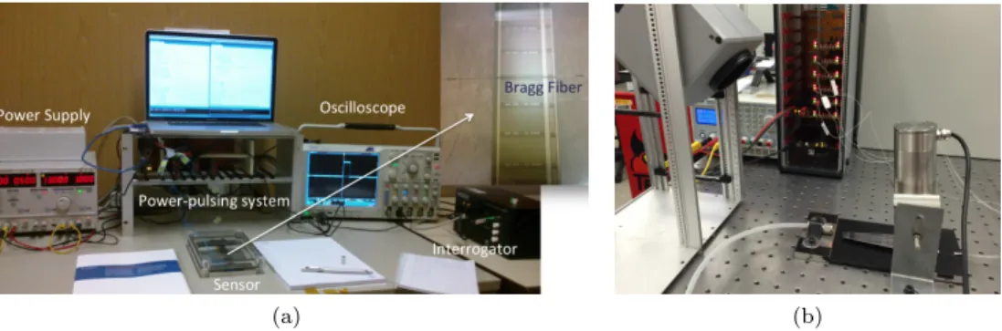
3.2.2 Experimental setup . . . 49
3.2.3 Thermo-mechanical performance . . . 50
3.3 Air flow cooling . . . 51
3.3.1 FTD mechanical support . . . 51
3.3.2 Experimental setup . . . 51
3.3.3 Thermo-Mechanical performance . . . 53
3.4 Integrated cooling channels in silicon detectors . . . 57
3.4.1 Microchannel circuits . . . 57
3.4.2 Connectors . . . 59
3.4.3 Finite Element Simulation . . . 60
3.4.4 Thermo-mechanical performance . . . 62
3.5 Summary . . . 66
4 Detector concepts, event generation, simulation and reconstruction 69 4.1 Detector concepts . . . 69
4.1.1 ILC detectors . . . 69
4.1.2 CLIC detectors . . . 71
4.2 Software . . . 72
4.2.1 Event Generation . . . 73
4.2.2 Full simulation of the ILD detector . . . 73
4.2.3 Event Reconstruction . . . 73
4.2.4 Backgrounds . . . 76
4.3 Summary . . . 79
5 Jet Reconstruction 81 5.1 Overview of jet reconstruction algorithms . . . 81
5.2 The VLC algorithm . . . 83
5.3 Comparison of the distance criteria . . . 85
5.4 Monte Carlo simulation . . . 87
5.4.1 Top quark pair production at a 500 GeV ILC . . . 87
5.4.2 Di-boson production at CLIC at√s= 500 GeV . . . 88
5.4.3 Higgs pair production . . . 89
5.4.4 Boosted top quarks at high-energy CLIC stages . . . 91
6 The Top Physics potential of Future Linear Colliders 97
6.1 Top quark production at e+e− colliders . . . . 97
6.2 A general Lagrangian . . . 100
6.3 Observables . . . 101
6.3.1 Cross section and forward-backward asymmetryAt F B . . . 101
6.3.2 OptimalCP-violating observables . . . 102
6.4 Monte Carlo simulation study . . . 104
6.4.1 Event selection . . . 104
6.4.2 Event reconstruction . . . 105
6.4.3 Statistical uncertainties . . . 108
6.4.4 CP-violating asymmetries . . . 108
6.5 Theory and systematic uncertainties . . . 111
6.6 Limits on form factors . . . 112
6.7 Summary and outlook . . . 115
Conclusions 117 Appendices 119 A Glossary 120 A.1 Acronyms . . . 120
A.2 Contributions . . . 122
A.2.1 Detector R&D . . . 122
A.2.2 Jet Reconstruction . . . 122
A.2.3 Top Physics . . . 122
B Standard Model formalism 124 B.1 Local Gauge Symmetries . . . 124
B.1.1 Quantum Electrodynamcis . . . 124
B.1.2 Quantum Chromodynamics . . . 124
B.2 Electroweak theory . . . 125
B.2.1 Charged and neutral currents . . . 126
B.2.2 Spontaneous Symmetry Breaking . . . 127
B.2.3 Higgs mechanism . . . 128
C Analysis of e+e−→tt¯and top quark form factors 130 C.1 Selection of tt¯events at 500 GeV . . . 130
C.2 Optimal observablesO±Re,ImandCP-violating asymmetries . . . 132
C.3 Generation of non-zero CP-violating couplings inMADGRAPH . . . 133
C.4 Covariance matrices . . . 136
Resumen 139
Bibliography 149
Chapter 1
The Standard Model of Particle
Physics and the Top Quark
1.1
Historical overview
The concept of elementary particles or elementary entities was proposed for the first time by ancient greeks under the name of atoms. However, the concept of indivisible components of matter evolved over time. In the second half of 19th century atomic spectra were studied by chemists and Mendeleiev established the well-known periodic table of elements in 18691.
1.1.1
The birth of the modern atom
Pioneering work at the end of the 19th century using cathode ray tubes, radioactive materials and photographic plates began the revolution that was to produce atomic physics. In 1895, W. C. Röntgen discovered an unknown radiation produced in cathode ray tubes which called X-rays. A year later, Becquerel observed that some materials, such as uranium, leave a signal on photographic plates due to its radioactive nature. Finally, J. J. Thomson interpreted cathode rays as ‘electrons’ and proposed a model of the atom consisting of a swarm of many of electrons with a balancing positive charge. The beginning of the new century was marked by Planck’s discovery of the black-body radiation law. The physical interpretation of this phenomenon led to postulate that energy was quantized. In 1905 Einstein used the Planck constant h to explain the photoelectric effect observed by Herz in 1887. Figure1.1 shows how illuminated metals emit electrons. The energy of the electrons depends on the frequency of the light, not on its intensity. Einstein’s explanation postulates that light of frequency ν
is composed of individual quanta -now known as photons- of energyhν.
1This section tries to introduce the reader in the world of particle physics in an informative way, from the first particle discovered in simple experiments to the huge particle colliders of the last decade. This historical review is based on References [1,2,3,4] where a more exhaustive description of the particle discoveries and experiments is done.
1.1. Historical overview 2
Figure 1.1: The photoelectric effect
Investigations of radioactivity performed by Geiger, Marsden and Rutherford in 1911, consisting in bombarding a thin metal foil withαparticles, proved that the atom
has a small nucleus with a charge Z|e|. Two years later Niels Bohr’s atomic model reproduced the electron energy levels and obtained the radius of the hydrogen atom, combining the electron massmeand electron chargeewithh. Afterwards Rutherford himself proved that the hydrogen nucleus was a fundamental constituent of all other nuclei. He broke a nitrogen nucleus with α particles and extracted hydrogen nuclei which were later called ‘protons’.
During the years 1924-1927, quantum mechanics developed rapidly, from de Broglie’s waves until Heisenberg’s matrix mechanics expressed in the Schrödinger’s equation and Dirac’s formulation of transition amplitudes. The problem of the electronic structure of the atom was reduced to a set of differential equations, approximations which ex-plained not just hydrogen, but all atoms.
Despite the progress, the structure of the nucleus remained a mystery. By 1926 it was understood that all particles were divided into two classes according to their intrinsic angular momentum, known as ‘spin’. Those with half-integer spin (in units of
}=h/2π) are called fermions, while those with integer spin are called bosons. These
fundamental facts about spin could not be reconciled with the prevailing picture of the nucleus N14
7 composed by 14 protons and 7 electrons. As these are both fermions the nucleus should be a fermion with half-integer spin, but it was shown to have spin 1. The nitrogen spin inconsistency and the enigma of the composition of the nucleus were solved with the discovery of the neutron by Chadwick in 1932. The experiment consisted in bombarding beryllium with α particles. He showed that the electrically neutral radiation that is produced in the process consisted of neutral particles with about the same mass as the proton, later called ‘neutrons’. The modern atom was completed. A nucleus with charge Z and mass number A is composed onZ protons
1.1. Historical overview 3
1.1.2
The leptons: beyond electrons
As discussed, the electron was the first elementary particle to be identified. In 1906, Millikan measured the electric charge by observing tiny charged droplets of oil between two horizontal metal electrodes. According to the theory developed by Pauli in 1927, the electron spin takes a value of 1/2. The electron therefore is the first element of a family of particles called ‘leptons’.
The positron, e+
Experiments using X-rays and radioactive sources were limited to energies of a few MeV. To obtain higher energy particles it was necessary to use cosmic rays, observed for the first time by V. Hess in 1912, who ascended by balloon with an electrometer to an altitude of 5000 m. Anderson, together with Millikan, studied cosmic-ray particles in a cloud chamber when he discovered the ‘positron’ in 1933, a particle with the same mass as the electron but the opposite charge. Just a few years before, Dirac’s relativistic wave equation for electrons had already predicted the existence of such a particle. Anderson’s positrone+, Thomson’s electron e− and Einstein’s photonγ
filled all the roles called for in Dirac’s relativistic theory. Muons,µ− and µ+
Anderson and Neddermeyer continued studying cosmic radiation. Anderson had ob-served a new penetrating component of the cosmic rays, particles that curved dif-ferently from electrons when passed through a magnetic field. They were negatively charged but curved less abruptly than electrons, but more abruptly than protons, for particles of the same velocity. To account for the difference in curvature, it was supposed that this kind of particles is heavier than an electron but lighter than a proton.
In 1935 Hideki Yukawa predicted the existence of a particle of mass intermediate between electron and proton, around 200 MeV/c2. This particle was to carry the nuclear force in the same way as the photon carries the electromagnetic force. It was thought initially that Anderson’s observation could be consistent with Yukawa’s particle. However, in late 1937, Street and Stevenson reported a track that ionized too much to be an electron with the measured momentum, but traveled to far to be a proton. The existence of the ‘muon’, µ, the second lepton, was confirmed. A decade
later, the group formed by Lattes, Occhialini and Powel discovered the pion, π(the
Yukawa-like particle), and explained the origin of the penetrating component of the cosmic rays using emulsions.
Electronic and muonic neutrinos (νe, νµ)
The discovery of the neutron was the key to understanding nuclearβ decay. However the problem of the energy non-conservation in some nuclear decay reactions remained. In order to explain this incongruence, in 1930, Pauli postulated the existence of a light, neutral, feebly interacting particle. It was later called ‘neutrino’, a name coined by Fermi, and was believed to be unobservable. At the time the decay of a neutron from
1.1. Historical overview 4 a nucleus was being considered as a 2-body process, n → pe, that implies a
mono-energetic electron signal rather than a continuous distribution. The success of the Fermi theory was convincing evidence for the existence of the neutrino. However, still there had been no detection of interactions by the neutrinos themselves until Cowan and Reines succeeded to observe them in an experiment made in 1956. They used the enormous number of antineutrinos produced inβ decays inside a nuclear reactor
and water with cadmium and scintillators as detector. The process νp¯ → e+n was observed by detecting both thee+ and the neutron.
The first theory of the neutron decay n → pe¯ν, now called ‘weak interaction’,
was proposed by Fermi in 1933. A 4-body point-like interaction without intermediate particle and including a coupling constant GF nowadays known as Fermi constant. During the next few years the universality of the theory became evident. It was suggested that the pairs (e, ν), (µ, ν) and (n, p) entered into the weak interaction in an equivalent way. Nuclear β decays and, pion and muon decays could be explained considering the interaction of these particle pairs.
Soon after, strong focusing led to the construction of much higher-energy proton machines. The Alternating Gradient Synchrotron (AGS) was completed at Brookhaven in 1960. In 1962, Schwarz, Steinberger and Lederman reported results where neutrino interactions were observed. The neutrino beam was generated by directing the 15 GeV proton beam of AGS to a beryllium target, where secondary kaon and pion de-cays produced the neutrinos. They observed that neutrinos from the beam could only produce muons but never electrons. This experiment showed that νe and νµ were distinct particles and there were two conserved quantum numbers, one for muons and another for electrons.
The third lepton, τ
In the following years the construction of e+e− storage rings became the way to go
ahead in particle physics. Fermion-antifermion pairs were expected to be produced in the e+e− annihilation, like the process e+e− → µ+µ−. However in 1975, a team
under M. Perl working in the MARK-I experiment of the e+e− colliding-ring SPEAR
at SLAC, observed events with a muon produced together with an electron of opposite charge and missing particles. They interpreted these events as the pair production of a new lepton, tau (τ), followed by its leptonic decays, τ →eνν andτ → µνν. The
third member of the leptons family was discovered. It is much heavier than the other leptons, and could only be produced in high energy collisions.
The tau neutrino, ντ
After theτ discovery there was no doubt about the existence of a third neutrino,ντ, but it took a long time to be observed. In 2000, an international collaboration of physicists at Fermilab, made the discovery after a three-year analysis of data from the Direct Observation of the Nu Tau (DONUT) experiment. The DONUT team fired an intense beam of neutrinos, which they expected to contain tau neutrinos, at a target consisting of iron plates with layers of emulsion sandwiched between them. One in 1012 tau neutrinos interacted with an iron nucleus to produce a tau lepton, which
1.1. Historical overview 5 subsequently decayed leaving a characteristic track in the emulsion that the team could identify. The lepton family had been completed, in today’s Standard Model it is composed by the particles (e, µ, τ) and (νe, νµ, ντ).
1.1.3
The era of quarks
Once Yukawa’s particle, the pion, was finally discovered, it was soon realized that protons, neutrons and pions were just the first members of a new family of particles. These hadrons differ from leptons, as they manifest strong interactions. This family is divided into two main groups: mesons, when the spin is integer, andbaryons, when the spin is half-integer. The development of more powerful particle accelerators and the measurement of the scattering cross sections uncovered new particles in the form of resonances, particles with extremely small lifetimes. As more particles and resonances were found, certain patterns appeared. It was known that the different processes observed at experiments had to conserve parity symmetry and conserve total angular momentum2. The discovery of the π0 completed the triplet of pions: π+, π0, π−.
The approximate equality of the charged and neutral pion masses had already been observed in the neutron and proton masses. It led nuclear physicists to postulate an approximate symmetry, the isotopic spin orisospin. Thus as the nucleons represent an isospin doublet, the pions represent an isospin triplet.
In 1953, the Cosmotron at Brookhaven National Laboratory provided an especially important result, the observation of four events in which a pair of unstable particles was produced. If the decays of these particles involved strong interactions, the particle lifetimes should have been ten orders of magnitude smaller than observed. They were called strange particles. The explanation of this unexpected result was given by Gell-Mann and Nishijima, introducing a new additive quantum number calledstrangeness. The eightfold way and u, d, squarks
Isospin symmetry could be represented by the neutron and proton, which has the mathematical structure of SU(2). Gell-Mann and Ne’eman proposed a model that
was an extension of SU(2) adding strangeness, a SU(3). Baryons and mesons were grouped in octets or combinations of them. It was called the “eightfold way”. In Figure1.2the baryon and meson octets are displayed. The discovery of a new baryon known asΩ−by Samios and collaborators in 1964, completed the decuplet of particles
with spin 3/2, shown in Figure1.3
A clearer understanding of SU(3) emerged when Gell-Mann and, independently, G. Zweig, proposed that hadrons were built from three basic constituents, “quarks”. Now called u(“up”), d (“down”) and s (“strange”), these could explain why the eightfold
way was so successful. Mesons were composed of a quark (q) and an antiquark (q¯)
while baryons are produced from three quarks. For instance, a proton is formed by the combination uud, a neutron byudd, whereas the meson K0 is a strange particle
2Total angular momentum, J, comes from the combined spin angular momentum, s, with the orbital angular momentuml; Parity,P, is defined as (-1)−l. Each particle has its ownJP numbers.
1.1. Historical overview 6
(a) (b)
Figure 1.2: The horizontal direction measuresIz, the third component of isospin. The
verti-cal axis measures the hyperchargeY =B+S, the sum of baryon number and strangeness. (a)
The baryonJP = 1/2+ octet containing the proton and the neutron. (b) The pseudoescalar
(meson) octet.
formed byd¯s. Quarks have spin 1/2 and fractionary charge, assigning a charge to the upquark of +2/3e(whereeis the electron charge) and -1/3eto the other two.
In the late 1960s, deep inelastic electron scattering became a powerful tool to explore nucleon constituents. An example is the experiment carried out by the SLAC-MIT groups, where they scattered electrons from a hydrogen target and detected the outgoing electrons in a large magnetic spectrometer. The most important result was the discovery of “scaling” behaviour, a concept anticipated by Bjorken in 1967. It suggested that experimentally observed strongly interacting particles (hadrons) be-have as collections of point-like constituents when probed at high energies. Scaling implied independence of the absolute resolution scale, and hence effectively point-like substructure. The observation of scaling by experiments at SLAC reinforced the faith in quarks as physical entities.
1.1. Historical overview 7 Richard Feynman subsequently formulated the parton model. In this picture there were three “valence” quarks in the nucleons that dominated the process of electron scattering, an in addition a “sea” of low-momentum antiquark pairs. The quark-parton model and the experimental confirmation, inspired the formulation of Quantum Chromodynamics (QCD). In this theory the interactions between quarks are the result of exchanging vector particles, called gluons, of spin 1. When a quark scatters, it emits gluons and some of its momentum is given to them. QCD adds a new quantum number, “colour”, with an SU(3) structure. Each parton came in three versions, i.e., red, blue and green.
The J/ψ resonance and thec quark
In 1974 the period known as the “November Revolution” began. The J and ψ
res-onances with 3.1 GeV mass were discovered simultaneously at Brookhaven National Laboratory and SLAC. Once it was realized that they had discovered the same par-ticle, the two teams agreed to name it J/ψ. This particle could not be understood without considering a fourth quark in addition to the original three, the “charmed” or c-quark. A c¯c bound state is the simplest way to explain the absence of neutral
strangeness-changing weak currents observed.
The new quark seemed to complete a family of fermions, (c, s, νµ, µ), analogously to (u, d, νe, e). As pointed out in the Section 1.1.2, during this exciting period of investigation, theτlepton was also discovered. Hence the third lepton and its neutrino
augured a new pair of quarks. Consequently, experiments were extended to search for the next quark.
The b quark
In 1977, the team under L. Lederman at Fermilab discovered the fifth quark, named “bottom” or “beauty”. They studied collisions of 400 GeV protons on nuclear targets. Their apparatus was a double-arm spectrometer intended to measure µ+µ− pairs. A
statistically significant peak was observed in the 9.5 GeV region and further analysis certified the discovery of a new resonance named Υ(ab¯bbound state). The story of
theJ/ψ was recurring. A year later the PLUTO and DASP II detectors in thee+e−
storage ring DORIS at DESY determined the mass of Υ with better precision and
extracted the charge of theb quark, -1/3.
Gluons
QCD postulated the dependence of the strong couplingαs, between quarks and gluons, on the momentum transferQ2. Corrections to the processe+e− →q¯qproducee+e−→ q¯qg, wheregis a gluon. The cross section for this is of order ofαsrelative to the process in which no gluon is produced. The q¯qg state could be produced at the SPEAR or DORIS rings, but higher energies were needed to distinguish the q¯qg from the qq¯, because both states merged. This was achieved first at PETRAe+e− collider located
at DESY, which was able to reach more than 30 GeV total center-of-mass energy. This ring had four detectors, TASSO, PLUTO, MARK-J and JADE. All of them
1.1. Historical overview 8 found evidence for the q¯qg final state. They observed that as energy increased, more
and more events with a gluon were produced. Some of the events displayed a clean three-jet3 topology, giving visual evidence for the existence of the gluon, as shown
Figure1.4.
30 (9.46 GeV) and the gluon discovery (a critical recollection of PLUTO results).
In June 1979, B. Wiik (TASSO) exhibited the first evidence of three jet-like events (a single event using only charged particles) at PETRA (Bergen Conference, [51]). Later at Geneva [45] P. Söding (TASSO) showed a few more events; all events were reconstructed yet without energy and momentum conservation.
PLUTO [49,50,53,57], and the other PETRA experiments confirmed [52,54,55] the presence of three exclusive jets. Figure 17 shows a PLUTO 3-jet event; in this case the availability of neutral energy data in the detector gave a significant contribution to reducing the systematic errors (see Fig. 17 from [50]). It should be noted that the gluon bremsstrahlung effect, even at the highest energies of PETRA has only a 10% probability, to be compared with the almost 97% direct to 3-gluon decay (according to QCD and confirmed experimentally by PLUTO). At this point at PETRA, a cross section was not yet measured.
Fig. 17. An evident 3-jet event (interpreted as ̅ ) from PLUTO data at PETRA: 13 charged tracks (8 vertex fitted) and 5 neutral clusters (out of 13 showers) were reconstructed. (The numbers are just labels: energy of showers and momentum of tracks are not shown here [50,53]).
Figure 1.4: An evident 3-jet event (interpreted asqqg¯) from PLUTO data at PETRA. [5]
The top quark
After these remarkable events, nobody doubted that the sixth quark must exist. Grouping the quarks in pairs (u, d) and (c, s) according to their charge, the
exis-tence of a sixth quark was necessary to complete the third pair together with the b,
thet quark or “top”. The race for discovering the top quark had started. However, it
took a long time until the top quark was directly seen for the first time. The discovery of theW andZ bosons, and the Standard Model (explained in Sections1.1.4and1.2) indicated where to search for the new quark. The top quark decay would be t→W b
and theW could decay leptonically (lν) or hadronically (q¯q). This, together with the
predicted mass around 180 GeV, was the key to discover the top quark in 1995 by the CDF and D∅ detectors operating at the 1.8 TeV Tevatronp¯pcollider at FERMILAB.
1.1.4
From neutral currents to the Higgs discovery
Fermi’s theory of weak interactions was based on the analogy with electromagnetism; from the start it was clear that there might be vector particles transmitting the weak force the way the photon transmits the electromagnetic force. Since the weak interac-tion is of short range, the vector particle would have to be heavy, and since β decay
3A jet is a narrow cone of hadrons and other particles produced by the hadronization of a quark or gluon.
1.1. Historical overview 9 changed nuclear charge, the particle would have to carry charge too. The weak (orW
boson) was the object of many searches. In 1961, Glashow developed a model that unified the weak and electromagnetic interactions. This model could accommodate particles like the photon and W+ andW−. In addition a new particle was required,
theZ boson, neutral like the photon, but heavy. The problem of this theory was that
all fields were gauge fields and therefore massless and unphysical.
An important advance was made by Peter Higgs and others, who in 1964 showed how a theory initially containing a massless photon and two scalar particles could turn into a theory with a massive vector particle and one scalar. This “Higgs mechanism” was adopted by Weinberg and Salam to complete Glashow’s model and develop the Standard Model of electroweak interactions (a detailed description is given in Section
1.2). The particles of this model were denotedW+,W−,W0andB. TheW’s conform the vector particles and B is the scalar. The Higgs mechanism gives mass to theW±
bosons, and at the same time, the two neutral particlesW0 andB mixed to produce two physical particles, a massless photon and aZ with a mass comparable to that of
theW±.
W and Z bosons
Neutral currents had been searched for in Kaon decays without success; they had to be very rare or nonexistent. The large electromagnetic effect always masked the neutral weak current in these processes. It was later realized how to avoid this. The idea was to look for scattering initiated by a neutrino that emitted aZ that subsequently
interacted with a nuclear target. Photons could not be emitted, as neutrinos are neutral. The discovery of neutral currents was made in 1973 in the Gargamelle bubble chamber at CERN. The experiment made use of muon antineutrino and neutrino beams. Just one event of the type νµe→νµe, shown in Figure1.5, without a final-state muon, was observed. Apart from finding evidence of neutral current events, the experiment measured later, with more statistics, the ratio of neutral to charged currents. This allowed to predict the masses of theW andZ bosons at about 80 and 91 GeV, respectively.
The promising theory of electroweak interactions encouraged to build higher en-ergy machines. A few years later, the CERN super proton synchrotron (SPS) was transformed into a proton-antiproton colliding machine according to the design by C. Rubbia and S. van der Meer, the Sp¯pS Collider. Quarks from protons colliding
with antiquarks from antiprotons could produce theW and theZ bosons at this new
powerful accelerator. For instance, if a uquark and a d¯quark collided, a W+ could be created if the energy of the pair was near the mass of the W. As expected, the
W and Z bosons were discovered, in 1983 and 1984 respectively, by the two large detectors, UA-1 and UA-2 at the Sp¯pS. They were detected via their leptonic decays:
W → lν and Z → l+l−, l being an electron or a muon. The measured masses are
in good agreement with previous predictions of the Standard Model. The W+, W−,
andZ bosons, together with the photon (γ), constitute the four gauge bosons of the
1.1. Historical overview 10
Figure 1.5: Neutral current event observed by the Gargamelle experiment at CERN. The Higgs boson
The Standard Model was still not complete. The Higgs mechanism required the exis-tence of a new boson, called Higgs boson. The first attempt to search for the Higgs boson was done at thee+e−collider Large Electron-Positron Collider (LEP) at CERN
in the 1990s. The Higgs boson could be produced through its gauge coupling to the Z, i.e.,e+e−→Z →ZH. The LEP searches did not find any conclusive evidence of a
SM Higgs boson. The data from the four detectors was combined and a lower bound on the Higgs mass was set at 114.4 GeV.
The search continued at Fermilab with the Tevatron proton-antiproton collider. There was no guarantee that the Tevatron would be able to find the Higgs boson because its mass remained unknown. The CDF and D∅ detectors were only able to exclude further ranges for the Higgs mass between 156 GeV and 177 GeV.
Years later the Large Hadron Collider (LHC) at CERN was built in the same 27 km tunnel where LEP was located, a proton-proton collider of up to 7 TeV of energy per beam. One of its goals was to confirm or exclude the existence of the Higgs boson. Collisions at these energy levels should be able to reveal it. Data collection at the LHC started in March 2010. At the end of 2011 the two main particle detectors, ATLAS and CMS had seen among their results an excess around 125 GeV that was becoming too large to ignore. Rapidly both experiments put their effort in finding the Higgs in the energy range around 115–130 GeV and again small but consistent excesses of events were observed across multiple channels. The decay modes observed with greatest significance were H → γγ and H → ZZ → 4 leptons. Finally, on 4 July 2012, ATLAS and CMS announced they had independently made the same discovery: an unknown boson of mass around 125-126 GeV with a local significance of 5σ. This level of evidence met the formal level of proof required to announce a
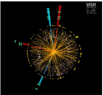
1.2. The Standard Model of particle physics 11 It is necessary to measure the properties of this new boson accurately to verify its Higgs-like nature. In 2013 the spin-parity of this particle was confirmed. The spin 0 and the even parity strongly indicated that it was a Higgs boson. Coupling measurements so far, with a precision ranging from 10 to 100%, are compatible with the Standard Model.
Figure 1.6: Event display of a (H → 4e) Higgs boson candidate from collisions in 2012
between protons in the ATLAS detector on the LHC.
After the Higgs discovery, the last piece of the puzzle, the Standard Model of par-ticle physics is complete. A theory that describes in a satisfactory way all interactions currently known, except gravity. In the following Section 1.2, the particle content, structure and symmetries of the Standard Model Lagrangian are presented.
1.2
The Standard Model of particle physics
The Standard Model constitutes one of the greatest achievements in modern physics. It provides an elegant theoretical framework, which is able to describe the known experimental facts in particle physics with high precision. It is a relativistic quantum field theory based on the symmetry groupSU(3)C⊗SU(2)L⊗U(1)Y, which describes strong, weak and electromagnetic interactions, via the exchange of spin-1 gauge fields. The development of the SM was driven by the interplay between theory and ex-periment. In spite of the impressive phenomenological success discussed in previous section, the SM leaves too many unanswered questions to be considered as a complete description of the fundamental forces. It does not incorporate the theory of gravitation as described by general relativity and does not contain any viable dark matter particle that possesses all of the required properties deduced from observational cosmology. It
1.2. The Standard Model of particle physics 12 also does not incorporate neutrino oscillations and non-zero neutrino masses. For this reason the SM is sometimes regarded as “the theory of almost everything” [2].
1.2.1
Particle content and interactions
All ordinary matter4 around us is made up of elementary particles. These particles
occur in two basic types called quarks and leptons. Each group consists of six particles, which are related in pairs or “generations”. The lightest and most stable particles make up the first generation, whereas the heavier and less stable particles belong to the second and third generations. All stable matter in the universe is made up of particles that belong to the first generation; any heavier particles quickly decay to the next most stable level. The six quarks are paired in the three generations, the
up and down quarks form the first generation, followed by the charm and strange
quarks, then the top and bottom (or beauty) quarks. Additionally quarks come in
three different “colours” and only mix in such ways as to form colourless objects. The six leptons are similarly arranged in three generations, the electron, the muon, the
tau and their respectiveneutrinos, as shown in Figure 1.7. The electron, the muon and the tau all have an electric charge and a sizable mass, whereas the neutrinos are electrically neutral and have very little mass.
Figure 1.7: The particle content of the Standard Model. On the left, fermions, the building blocks of matter, are subdivided into three families of quarks and leptons. On the right, vector bosons that carry the electromagnetic, weak and strong forces. In the middle, the Higgs boson, responsible for providing mass to all massive particles.
There are four fundamental forces at work in the universe: the strong force, the weak force, the electromagnetic force, and the gravitational force. They act over differ-ent ranges and have differdiffer-ent strengths. Gravity is the weakest, but is a far-reaching interaction. The electromagnetic force is far-reaching as well, but it is many times
4The standard model of cosmology indicates that the total mass–energy of the universe contains 4.9% ordinary matter, 26.8% dark matter and 68.3% dark energy [6]
1.2. The Standard Model of particle physics 13 stronger than gravity. The weak and strong forces are effective over a very short range and dominate only at the level of subatomic particles. Despite its name, the weak force is much stronger than gravity, but it is indeed the weakest of the other three. The strong force, as the name suggests, is the strongest of all four fundamental in-teractions. Three of the fundamental forces result from the exchange of force-carrier particles, which belong to a broader group called “bosons”. Particles of matter transfer discrete amounts of energy by exchanging bosons with each other. Each fundamen-tal force has its own corresponding boson, the strong force is carried by the gluon,
the electromagnetic force is carried by the photon, and the W± and Z bosons are
responsible for the weak force.
The fifth boson is the Higgs boson, associated with the Higgs field which gives mass to leptons (except neutrinos), quarks,W andZ bosons, and the Higgs boson itself.
1.2.2
Local gauge symmetries
Gauge theories and symmetry principles provide us with a comprehensive description of the presently known fundamental particles and interactions. The SM is based on gauge theories, and the interactions between the elementary particles are governed by a symmetry principle, namely local gauge invariance, which represents an infinite dimensional symmetry group. Global symmetries, such as isospin, or flavour symme-try, are only approximate symmetries and therefore they are not connected to gauge interactions. There is no explanation available for this rule, but gauge interactions play a fundamental role in our present understanding of particle interactions. The mathematical formalism of local gauge symmetries is detailed in AppendixB.1. a) Quantum electrodynamics
The simplest example of local gauge theory is Quantum Electrodynamics (QED), the quantum field theory of the electromagnetic force. QED mathematically describes all phenomena involving electrically charged particles interacting by means of exchange of photons and represents the quantum counterpart of classical electromagnetism giving a complete account of the interaction between matter and light.
QED is an abelian gauge theory with the symmetry group Uem(1) and has one gauge field, the electromagnetic four-potential, with the photon being the gauge boson. The Lagrangian of QED predicts the massless nature of photons. Experimentally we knowmγ <1×10⁻¹⁸eV [3].
In QED, the coupling constant that determines the strength of the electromagnetic interactions is known as the fine-structure constant, α = 4πe20}c. The SM does not
predict its value. Therefore, αmust be determined experimentally. In fact, αis one
of the about 20 empirical parameters in the SM. The most stringent QED test comes from the high-precision measurement of the e and µ anomalous magnetic moments
al ≡(gγl −2/2), where l =e, µ. The values of ae ≈10−12 and aµ ≈10−10 are fully compatible with predicted value of the gyromagnetic factorglγ= 2by the Dirac
1.2. The Standard Model of particle physics 14 the fine-structure constant [3]
α−1= 137.035 999 074±0.000 000 032 (1.1)
The impressive precision of this value promotes QED to the level of one of the most precise theories ever built to describe nature.
b) Quantum chromodynamics
As discussed earlier, mesons areM ≡q¯qstates, while baryons have three constituents, B ≡qqq. However, in order to satisfy the Fermi-Dirac statistics5, one needs to assume
the existence of a new quantum number,colour, such that each species of quark may
have NC= 3different colours: (red, green, blue).
There is no evidence of extra states with non-zero colour, thus to avoid this one needs to further postulate that all asymptotic states are colourless. This assumption is known as quark conf inement: since quarks carry colour they are confined within
colour-singlet bound states.
Experimentally the colour quantum number is tested through the measurement of the ratio [1]:
Re+e−≡ σ(e
+e−→hadrons)
σ(e+e−→µ+µ−) (1.2)
The production of hadrons occurs through e+e− → γ∗, Z∗ → q¯q → hadrons.
Since quarks are assumed to be confined, the probability to hadronize is just one. Therefore, one can estimate the inclusive cross-section into hadrons summing over all possible quarks in the final state. The electroweak production factors which are common with the e+e− →γ∗, Z∗ →µ+µ− process cancel in the ratio. At energies
well below the Z peak, the cross-section is dominated by theγ-exchange amplitude
and the ratioRe+e− is then given by the sum of the quark electric charges squared:
Re+e− ≈NC Nf X f=1 Q2f = 2 3NC = 2, (Nf = 3 : u, d, s) 10 9 NC = 10 3 , (Nf = 4 : u, d, s, c) 11 9 NC = 11 3 , (Nf = 5 : u, d, s, c, b) (1.3)
This formula involves an explicit sum over theNf quark flavours multiplied by the number of different colour possibilities NC, taken to be three. Notice that the top quark is not included, as its mass is larger than the Z mass. The measured ratio is
shown in Figure 1.8. The simple rule in Equation1.3 provides a good description of the observed behaviour of Rover a broad range of energies. Thus it seems natural to
5Fermions obey a statistical rule described by Fermi, Dirac and Pauli called the “exclusion princi-ple”. No two fermions may be described by the same quantum numbers.
1.2. The Standard Model of particle physics 15 take colour as the charge associated with the strong forces and try to build a quantum field theory based on it. That theory is known as QCD.
10 -1 1 10 102 103 1 10 102
R
ω ρ φ ρ′ J/ψ ψ(2S) Υ Z√
s
[GeV]
Fig. 3: World data on the ratioRe+e− [9]. The broken lines show the naive quark model approximation with
NC= 3. The solid curve is the 3-loop perturbative QCD prediction.
2.2.2 Non-Abelian gauge symmetry Let us denoteqα
f a quark field of colourαand flavourf. To simplify the equations, let us adopt a vector notation in colour space:qTf ≡ (qf1, qf2, q3f). The free Lagrangian
L0 =
! f
¯
qf (iγµ∂µ−mf)qf (19)
is invariant under arbitraryglobalSU(3)Ctransformations in colour space,
qfα −→ (qαf)′ = Uαβqfβ, U U† = U†U = 1, detU = 1 . (20)
TheSU(3)C matrices can be written in the form
U = exp " iλ a 2 θa # , (21) where 1
2λa (a = 1,2, . . . ,8) denote the generators of the fundamental representation of theSU(3)C algebra,θaare arbitrary parameters and a sum over repeated colour indices is understood. The matrices
λaare traceless and satisfy the commutation relations $ λa 2 , λb 2 % = i fabc λ c 2 , (22)
withfabctheSU(3)C structure constants, which are real and totally antisymmetric. Some useful prop-erties ofSU(N)matrices are collected in Appendix B.
As in the QED case, we can now require the Lagrangian to be also invariant underlocalSU(3)C transformations, θa = θa(x). To satisfy this requirement, we need to change the quark derivatives by covariant objects. Since we have now eight independent gauge parameters, eight different gauge bosons Gµa(x), the so-calledgluons, are needed:
Dµqf ≡ $ ∂µ+igsλ a 2 G µ a(x) % qf ≡ [∂µ+igsGµ(x)]qf. (23) 5
Figure 1.8: World data on the ratioRe+e−[7]. The broken lines show the naive quark model
approximation with NC = 3. The solid curve is the 3-loop perturbative QCD prediction.
QCD is represented by the symmetry groupSU(3)c, the gauge group of the colour triplets, and the gluon is the associated gauge boson. The SU(3)C gauge symmetry forbids to add a mass term for the gluon fields because it is not invariant under the local transformation. Gluons are, therefore, massless spin-1 particles.
Properties of QCD
• All interactions are given in terms of a single universal couplinggs, which is called thestrong coupling constant, commonly defined asαs= g
2
s
4π. Experimentally, the value of the coupling constant is determined as αs(MZ2) = 0.1185 [3] at MZ energy escale. Cubic (g3s) and quartic g4s gluon self-interactions are allowed in QCD.
• The phenomenon known asasymptotic freedomimplies that the strong force
be-tween quarks becomes weaker at short distances, but increases at large distances, a property known as thequark confinement.
• At high-energy collisions in a particle collider, “free” quarks or gluons might be created. Due to the colour confinement, these cannot exist individually. They combine with quarks and antiquarks spontaneously created from the vacuum to form hadrons. This process is called hadronization. The tight cone of particles created by the hadronization of a single quark is called a jet.
1.2. The Standard Model of particle physics 16
1.2.3
Electroweak unification
Weak interactions are distinguished from QED and QCD by some characteristic prop-erties like lifetimes, strength of coupling, cross-sections, and violation of symmetries. These interactions are short-ranged, which requires massive messenger particles, seem-ingly inconsistent with gauge invariance. They come in two types, charged and neutral current interactions, which couple quarks and leptons differently. Charged current in-teractions, mediated by theW± bosons, only involve left-handed fermions and readily
change flavour, as in the strange quark decay s → ue−ν¯e. Neutral current interac-tions mediated by theZ boson, on the other hand, couple both left- and right-handed
fermions, and flavour-changing neutral currents are strongly suppressed.
To describe electroweak interactions, one needs a more elaborate structure than QED or QCD Lagrangians. The EW theory is a “chiral” gauge theory6, hence the
building blocks are massless left- and right-handed fermions. The electroweak gauge group is a product of two groups,GEW ≡SU(2)L⊗U(1)Y. The non-Abelian group
SU(2)L is associated to the “weak isospin” quantum number and theU(1Y)charge is the weak hyperchargeY, which is related to the electric chargeQby
Q=I3+
Y
2 (1.4)
where I3 is the third component of the weak isospin. In the weak interactions only the left-handed components couple to the SU(2)L gauge field. This suggests to form doublets from quarks uL and dL, and leptons eL and νL, keeping the right-handed fields as singlets. HenceSU(2)L multiplets can be represented as follows:
qL= u L dL , uR, dR, lL= ν L eL , eR, (1.5) where the right-handed neutrino is omitted because it is not part of the SM. The EW theory generates four gauge bosons which can be identified by the physical bosons
W+, W−, Z and γ and establishes the following relation between the SU(2) L and
U(1)Y couplings to the electromagnetic coupling:
gsinθW =g0cosθW =e, (1.6) whereθW is the Weinberg or weak mixing angle,gandg0are the couplings constants of the charged and neutral currents, andeis the electromagnetic constant coupling. This
relation provides the unification of the electroweak interactions. The mathematical formalism of the EW theory and its Lagrangian are presented in AppendixB.2.
The Lagrangian in EquationB.14describes mathematically the interaction between fermions (quarks and leptons) and gauge bosons. It allows to deduce expressions for the fermion couplings to Z and γ bosons as a function of their charge and isospin
quantum numbers. These expressions are shown in Table1.1. Note that members of
6In quantum field theory, a chiral gauge theory is a quantum field theory with charged chiral fermions. The electroweak model breaks parity maximally, which means that the charged weak gauge bosons only couple to left-handed quarks and leptons while the neutral electroweakZboson couples to both left- and right-handed fermions
1.2. The Standard Model of particle physics 17 Table 1.1: Neutral-current couplings of quarks and leptons toZ andγbosons Couplings (u, c, t) (d, s, b) (νe,νµ, ντ) (e, µ,τ)
2vf 1−83sin2θW −1 + 43sin2θW 1 −1 + 4 sin2θW
2af 1 -1 1 -1
the same family have the same values of Qf and I3f, for instance Q(u,c,t) = 2/3 and
I3(u,c,t) = 1/2. The top quark couplings to Z and γ are the main topic of this thesis. In Chapter6 an analysis of the process e+e− →Z/γ → t¯t is presented, that allows
the extraction of these electroweak couplings.
1.2.4
Spontaneous Symmetry Breaking
The physicalZ andW± bosons have a non-zero mass, which is forbidden by the local
gauge symmetry of the groupGEW. That incongruence is solved through Spontaneous Symmetry Breaking (SSB), a mechanism that generates masses for the gauge bosons and fermions without destroying gauge invariance. In the SM this mechanism is known as theHiggs mechanism. It allows to match the spontaneous symmetry breaking by vacuum with the massless Goldstone bosons7. The Higgs mechanism makes a clever
use of local gauge symmetry, converting massless gauge bosons into massive ones and explains why theW± andZ bosons are massive. In a similar way, fermion masses are
also generated. The mass of each particle will depend on how strong it interacts with the Higgs field. A mathematical formulation of the SSB and the Higgs mechanism is given in AppendixB.2.2.
1.2.5
Experimental particle masses
The SM does not predict the values of some of its parameters. These parameters and their values have to be established by experiment. Among these parameters one can find the masses of the leptons and quarks, the Higgs boson mass or the gauge couplings
g, gS, g0. Tables1.2and1.3list the measured values of the fundamental SM particles. The SSB mechanism yields a precise prediction for theW±andZmasses, relating
them to the vacuum expectation value v of the Higgs boson through the Eq. B.25.
Thus,MZ is predicted to be larger thanMW, in agreement with the measured masses in Table1.2[3].
From experiment, one obtains the electroweak mixing angle
sin2θW = 1− M2 W M2 Z = 0.023. (1.7)
One can estimate the Weinberg angleθW from the muon decayµ−→e−ν¯eνµ. Due
7Goldstone bosons are spin-0 bosons that appear necessarily in models exhibiting spontaneous breakdown of continuous symmetries.
1.2. The Standard Model of particle physics 18 Table 1.2: Experimental mass and charge of the gauge bosons. Values taken fromReview of Particle Physics, Particle Data Group [3].
Bosons γ gluon W Z H
Mass[GeV] <10−27 0 80.385
±0.015 91.1876±0.0021 125.09±0.24 Q[e] <10−35 0
±1 0 0
to the large mass of the W propagator, the decay can be well approximated through
a local four-fermion interaction, i.e.,
4πα sin2θWMW2
= 4√2GF (1.8)
whereGF is the Fermi coupling constant. The most precise determination of its value is provided by the measured muon lifetime from [8]
GF = (1.166 378 8±0.000 000 7)·10−6 GeV−2 (1.9)
Therefore the precisely measured values of the QED coupling constant α, MW and
GF imply
sin2θW = 0.215, (1.10)
in rough agreement with the value obtained from theZ andW masses. The difference
is explained by higher order corrections, as explained in next Section1.2.6. Addition-ally, the Fermi constant gives a direct determination of the electroweak scale, i.e., the scalar vacuum expectation value:
v=√2GF −1/2
= 246GeV (1.11)
The experimental limit on the photon mass is totally compatible with the predicted massless boson by the SM. Also the gluon is theoretically massless, however a mass as large as a few MeV cannot be excluded. The experimental mass of the Higgs boson comes from the combined fit of the ATLAS and CMS experiments data at 7-8 TeV collisions at the LHC [9].
Unlike the leptons, quarks are confined inside hadrons and are not observed as physical particles. Quark masses therefore can not be measured directly, but must be determined indirectly through their influence on hadronic properties. Table1.3(a) shows experimental values for the quark masses. Any quantitative statement about the value of a quark mass must make careful reference to the particular theoretical frame-work that is used to define it. Thus it is important to keep this scheme dependence in mind. The most commonly used renormalization scheme for QCD perturbation theory is the modified minimal subtraction, or MS, scheme [11].
It is a well-known experimental fact that the neutrinos and antineutrinos are of three light varieties or flavours: (νe, νµ, ντ). The SM describes them as left-handed massless fields. However, experiments with solar, atmospheric, reactor and accelerator
1.2. The Standard Model of particle physics 19 Table 1.3: Experimental mass and charge of the elementary fermions. Theu,dands-quark
masses are estimates of so-called “current-quark masses”, in a mass-independent subtraction
scheme such as MS. Thecandb-quark masses are the “running” masses in the MS scheme.
For theb-quark the 1S mass is also quoted. Finally thet-quark mass is the pole mass from
the world combination of Tevatron and LHC measurements [10].
(a)
Quarks Mass [GeV] Q[e]
u (2.3 +0−0..75 )·10−3 2/3 d (4.8 +0−0..53 )·10−3 -1/3 s (95±5)·10−3 -1/3 c 1.275±0.025 2/3 b MS1S: 4.66: 4.18±0.03 ±0.03 -1/3 t 173.34±0.27±0.71 2/3 (b)
Leptons Mass [MeV] Q[e]
e ±0.5109989280.000000011 −1 νe 2·10−6 0 µ 105.6583715±0.0000035 −1 νµ <0.19 0 τ 1776.86±0.12 −1 ντ <18.2±0.48 0
neutrinos have provided compelling evidence for the existence of neutrino oscillations, transitions in flight between the different flavour neutrinos, only explicable by non-zero neutrino masses and neutrino mixing. There are ways to incorporate small non-zero neutrino masses (and lepton-flavor violation) through a lepton mixing matrix. For instance, if sterileνR fields are included in the model, one has an additional Yukawa term in equationB.28, giving rise to a neutrino mass matrixmν=λν√v2.
1.2.6
QED and QCD corrections
The increasing precision of experimental data in elementary particle physics requires an equally precise theoretical description. Quantum field theories are solved using perturbative expansions. In QED, for instance, any observable can be written as:
O=O0+αO1+α2O2+α3O3+..., (1.12) whereO0 corresponds to the observable at tree level andαnOn (withn >0) denotes the nth-order correction to the observable. Therefore, corrections described by one-and multi-loop Feynman diagrams have to be considered. They got the name of radiative corrections, since in QED they correspond to the emission and absorption of photons. One-loop Feynman diagrams of QED are shown in Figure1.9.
The first order of QCD corrections are commonly named as next-to-leading-order (NLO) and higher-order corrections as NnLO, withnbeing the number of loops con-sidered in Feynman diagrams.
In calculations in QED and QCD one finds two problems, the ultraviolet and the infrared divergences. One can get rid of these divergences and obtain finite corrections to the cross-sections of elementary processes using a technique called renormalisation.
1.2. The Standard Model of particle physics 20
Figure 1.9: Divergent first-order loops of QED
The infinite terms can be reabsorbed within the constants of the theory. For example, in QED divergences are reabsorbed withinαandme:
α(Q2) =α 0 1 + α0 3πf Q2 m2 e +O(α2 0) , (1.13)
whereα0is the “primary” constant appearing in the Lagrangian andα(Q2)the “renor-malized” value that should merge with the measured value. The functionf(Q2/m2
e)is the finite correction which causes the coupling to run with the energy scaleQ2. The resulting QED running coupling α(Q2) decreases at large distances (decreasingQ2). This can be intuitively understood as the charge screening generated by the virtual fermion pairs, shown in Figure 1.9 (c). It turns out that the effect is really small and can safely be ignored at atomic or nuclear scales. Nevertheless, it gives rise to a significant difference between the constant evaluated at electron andZ mass scales [3]
α(m2e)−1= 137.035 999 074±0.000 000 032 > α(MZ2)−1= 128.95±0.05 (1.14)
For Q2 >> m2
e the correction function can be approximated to f(Q2/m2e) ≈ ln(Q2/m2 e)8. α(Q2) = α0 1 +β0α0ln(Q2/m2e) with β0=− 1 3π (1.15)
This result is not exact, and is known as the leading log (LL) approximation. Additionally, there are corrections that imply more complicated propagator diagrams like multi-photon exchange between loops, not discussed here.
To calculate the propagator loop correction in QCD, one does not only have to consider quark loops such as these in left diagram of Figure 1.10, like electron loops in QED, but also gluon loops shown in right diagram of Figure 1.10. The quark loop gives rise to a positive contribution to theβ function (screening) while the gluon loop
contribution is negative (anti-screening).
Since the reference scaleQ2= 0cannot be used in QCD, one has to specify an input valueQ2(µ2)at some arbitrary reference scaleµ2. It is known as the renormalisation
81 +X+X+X3+...= 1 1+X
1.2. The Standard Model of particle physicsThe running strong coupling constant ↵s 21
( a ) ( b )
•To calculate the propagator loop correction in QCD, we do not only have to consider quark loops (a), like electron loops in QED, but also gluon loops (b). The quark loop will give rise to a positive contribution to the beta function (screening) while the gluon loop contribution will be negative (antiscreening), see also the discussion on charge screening on page 6–4.
•The formula for the one-loop running coupling constant in QCD is
↵s(Q2) = ↵s(µ2) 1 + 0↵s(µ2) ln(Q2/µ2) with 0= 11Nc 2nf 12⇡
Here Nc is the number of colours (3) and nf is the number of flavours (6 in the standard model).
•The second factor 2nf/12⇡in 0 comes from diagram (a). It is
the same (modulo a colour factor) as the coefficient 0 = 1/3⇡
in QED and causes screening. The first factor 11Nc/12⇡ comes
from diagram (b) and causes anti-screening.
•Clearly withNc= 3 andnf = 6, the antiscreening wins over the screening, with 0 > 0 and a slope (↵s) = 0↵2s < 0. This
means that↵s decreases withQ2(!fig).
6–16
g
g
g
g
g
g
q
Figure 1.10: QCD first-order loops.
scale. Hence, analogously to QED, the formula for the one-loop running coupling constant in QCD is αs(Q2) = αs(µ2) 1 +β0αs(µ2)ln(Q2/µ2) with β0= 11Nc−2Nf 2π , (1.16)
whereNcis the number of colours (3) andNf is the number of flavours (6 in the SM). The expression for the running coupling constant can be simplified when we define the QCD scale parameterΛas follows:
αs(Q2) = 1
β0ln(Q2/Λ2) (1.17)
For Q2 = M2
Z, the value of αs is of the order of 0.12. At this energy only five quarks can be excited inside the loops. This value implies thatΛ≈200MeV. Figure
1.11shows how the strong coupling constantαsdecreases with the energy scaleQ.
QCD αs(Mz) = 0.1181 ± 0.0013
pp –> jets
e.w. precision fits (NNLO)
0.1 0.2 0.3
α
s(Q
2)
1 10 100Q [GeV]
Heavy Quarkonia (NLO)
e+e– jets & shapes (res. NNLO)
DIS jets (NLO)
October 2015 τ decays (N3LO) 1000 (NLO pp –> tt(NNLO) ) (–)
Figure 1.11: Summary of measurements ofαs as a function of the energy scaleQ[3]. The
respective degree of QCD perturbation theory used in the extraction of αs is indicated in
brackets (NLO: next-to-leading order; NNLO: next-to-next-to leading order; res. NNLO:
1.3. The Top Quark 22
1.2.7
CP
violation
While parity and charge conjugation are violated by the weak interactions in a maximal way, the product of the two discrete transformations is still a good symmetry of the gauge interactions. In fact, CP appears to be a symmetry of nearly all observed phenomena. However, a slight violation of the CP symmetry at the level of 0.2% is observed in the neutral kaon system and more sizable signals of CP violation have been recently established at the B factories [12].
DirectCP violation is allowed in the Standard Model if a complex phase appears in
the Cabibbo-Kobayashi-Maskawa (CKM) matrix describing quark mixing. The CKM matrix couples any ‘up-type’ quark with all ‘down-type’ quarks. The ‘standard’ CKM parametrization is: V = VVudcd VVuscs VVubcb Vtd Vts Vtb It is described by three angles and one phase
V = c12c13 s12c13 s13e −iδ13 −s12c23−c12s23s13eiδ13 c12c23−s12s23s13eiδ13 s23c13 s12s23−c12c23s13eiδ13 −c12s23−s12c23s13eiδ13 c23c13 , (1.18)
wherecij ≡cosθij andsij ≡sinθij, withiandj the number of the quark generation
(i, j= 1,2,3).
A necessary condition for the appearance of the complex phaseδ13is the presence of at least three generations of quarks. In fact, it was for this reason that the third generation was assumed to exist, before the discovery of the band the τ. With only
two generations, the SM could not explain the observedCP violation in theK system
(∼2×10⁻³). In that system,
CP violation effects can only appear at the one-loop
level, where the top quark is present.
CP violation has not been observed in the top quark sector. Precision
measure-ments lead us to predict very small effects in the SM, but extensions could lead to non-negligible effects. Future e+e− colliders have the potential to measure that
phe-nomenon through the study of the t¯t production process. In the Chapter6, sensitive
observables toCPviolation effects in top quark decays are investigated in the ILC and CLIC environments.
1.3
The Top Quark
This section is dedicated exclusively to the top quark, the particle that is the focus
of this thesis. The top quark was discovered at the CDF and D∅ experiments at the Tevatron. Apart from the top quark mass and the CKM matrix elements, the SM predicts all properties of top quarks and their decays with high precision. Since the top quark lifetime is much shorter than the time required for hadronization, top quark properties can be measured directly and usually with much less uncertainty than
1.3. The Top Quark 23 those for other quarks, where these characteristics are derived from their bound states. Differences between measured properties and the precisely known SM predictions offer sensitive tests for new physics beyond the SM.
1.3.1
Top quark properties
The top quark is the heaviest known elementary particle, even heavier than the Higgs boson. Its large mass is the reason for its very short lifetime. In the SM the top quark has the same quantum numbers and interactions as all other up-type quarks. It is the weak isospin partner of thebquark with spin1/2 and electric chargeQt= +2/3. The left-handed top quark is the upper component of the weak isospin doublet and the right-handed component is a weak isospin singlet. It is a colour triplet with respect to theSU(3)Cgauge group. From the theory side, the top quark is absolutely needed to ensure cancellation of the chiral anomaly in the SM and therefore to ensure its consistency as a quantum field theory. An accurate knowledge of its properties (mass, couplings, production cross section, decay branching ratios, etc.) can bring key information on fundamental interactions at the electroweak breaking scale and beyond.
Top quark mass and lifetime
Measurements of the top quark mass, mt, using kinematic properties of the decay products of the top quark, i.e., using direct approaches, have been performed by the ATLAS, CDF, CMS, and D∅Collaborations using a variety of experimental techniques. The first world combination of mt measurements was performed in 2014 [10] and taking into account the correlations between the colliders, experiments, and analysis channels for all sources of systematic uncertainty considered. The combined value is
mt= 173.34±0.27(stat)±0.71(syst)GeV, which corresponds to a relative uncertainty
of 0.44%. The latest results from averaged 7-8 TeV data at CMS get even a more precise measurement∼0.5 GeV [13]. Expectations range from a pessimistic 500 MeV after the
complete LHC program to 200 MeV. These prospects do not include the uncertainty in the interpretation of the direct mass measurement as the pole mass [14]. On the other hand the most precise measurement of the top quark pole mass to date, with data collected by ATLAS at 7 TeV and luminosity of 4.6 fb−1, is found in Reference [15]. They show that the normalized differential cross section of thett¯+ 1jetsystem
as a function of its invariant mass can be used for a precise measurement of the top quark mass using the pole-mass scheme at NLO theoretical accuracy in QCD.
The lifetimeτand the related resonance widthΓ = 1/τ are primary characteristics
of any particle. A small value of the top lifetimeτtis expected due to its large mass and the large value ofVtb. The width of the top quark is computed in the SM to be 1.32 GeV with about 1% uncertainty [16] which translates into a top quark lifetime of (τt ≈ 5×10⁻²⁵s) that is much smaller than the typical time for formation of QCD bound state hadrons (τQCD ≈ 1/ΛQCD ≈ 3 ×10⁻²⁴s). Therefore hadrons containing a top quark are not expected to exist. It is impossible to measure such a short lifetime directly by measuring the distance between creation and decay. An alternative approach used for strongly interacting decays is the measurement of the
![Figure 1.11: Summary of measurements of α s as a function of the energy scale Q [3]. The respective degree of QCD perturbation theory used in the extraction of α s is indicated in brackets (NLO: next-to-leading order; NNLO: next-to-next-to leading order; r](https://thumb-us.123doks.com/thumbv2/123dok_us/10111585.2911730/33.748.157.570.589.853/summary-measurements-function-respective-perturbation-extraction-indicated-brackets.webp)
![Table 2.2: Luminosity and running time of the G-20, H-20, I-20 and Snowmass scenarios [44].](https://thumb-us.123doks.com/thumbv2/123dok_us/10111585.2911730/45.748.125.596.726.915/table-luminosity-running-time-g-h-snowmass-scenarios.webp)