Received 27 June 2014, Accepted 17 December 2014 Published online 1 February 2015 in Wiley Online Library (wileyonlinelibrary.com) DOI: 10.1002/sim.6413
Correcting for bias in the selection and
validation of informative diagnostic tests
David S. Robertson,
a*†A. Toby Prevost
band Jack Bowden
aWhen developing a new diagnostic test for a disease, there are often multiple candidate classifiers to choose from, and it is unclear if any will offer an improvement in performance compared with current technology. A two-stage design can be used to select a promising classifier (if one exists) in stage one for definitive validation in stage two. However, estimating the true properties of the chosen classifier is complicated by the first stage selection rules. In particular, the usual maximum likelihood estimator (MLE) that combines data from both stages will be biased high. Consequently, confidence intervals andp-values flowing from the MLE will also be incorrect. Building on the results of Pepeet al.(SIM 28:762–779), we derive the most efficient conditionally unbiased estimator and exact confidence intervals for a classifier’s sensitivity in a two-stage design with arbitrary selection rules; the condition being that the trial proceeds to the validation stage. We apply our estimation strategy to data from a recent family history screening tool validation study by Walteret al.(BJGP 63:393–400) and are able to identify and successfully adjust for bias in the tool’s estimated sensitivity to detect those at higher risk of breast cancer. © 2015 The Authors.Statistics in Medicinepublished by John Wiley & Sons Ltd.
Keywords: diagnostic tests; group sequential design; family history; uniformly minimum variance unbiased estimator
1. Introduction
The development and validation of an informative diagnostic test for a medical condition is of great use for clinicians. This process is well described in the literature if only a single diagnostic variable is studied. However, there are often multiple candidate classifiers that show potential as diagnostic tools, and it may also be unclear if any will offer an improvement compared to current technology. The challenge is to identify themostpromising diagnostic test and then to correctly validate its properties.
It is in the context of biomarker research that this challenge is particularly evident, where new tech-nological advancements have led to an abundance of biomarker discovery studies and a huge number of candidate markers, for example, in colorectal cancer [1] and prostate cancer [2]. Guidelines have also been established for the discovery and validation of potential biomarkers [3].
The development of questionnaires for diagnosis is a parallel endeavour to biomarker discovery and validation. There will be a set of possible questions, with each considered a candidate classifier. In particular, questions about the family history of a disease are simple and cheap to measure when com-pared with genetic or biomarker variables. They can also provide the bulk of a diagnostic or risk prediction tool’s classification ability, despite the discovery of many genetic markers [4].
To make efficient use of resources, a sequential procedure is a natural choice for the selection and validation of diagnostic tests. This is particularly the case for biomarkers, due to the high false discovery rate – despite showing initial promise, the majority of markers will not subsequently perform well enough compared with an existing test to be considered for further development. Also, many biomarker studies rely on stored biological samples, and there is a need to preserve specimen resources [5]. Hence, group sequential designs have been proposed that allow for early stopping because of poor marker performance
aMRC Biostatistics Unit, Institute of Public Health, Cambridge, UK
bKing’s College, London, UK
*Correspondence to: David S. Robertson, MRC Biostatistics Unit, Institute of Public Health, Robinson Way, Cambridge CB2
0SR, UK.
†E-mail: [email protected]
This is an open access article under the terms of the Creative Commons Attribution License, which permits use, distribution and reproduction in any medium, provided the original work is properly cited.
[5, 6]. In these settings, the simplest (two-stage) group sequential design has been proposed; whereby the discovery and validation phases are separated by a single interim analysis.
Estimating the performance of the chosen classifier is complicated by the first stage selection rules. A candidate classifier will have to perform well in the first stage in order to proceed to the validation stage, which will lead to overly optimistic estimates. In particular, the usual maximum likelihood estimator (MLE) that combines data from both stages will be biased high. Hence, hypothesis-testing procedures using the MLE will have incorrect p-values, with an inflation of the type I error rate. Furthermore, confidence intervals will have coverage probabilities that can be well below the nominal level.
There are obvious parallels in this endeavour with multi-arm adaptive clinical trials of pharmaceuti-cal treatments, where a promising single treatment or treatment dose is selected in a preliminary phase for a subsequent confirmatory analysis against standard therapy. Specific examples include seamless designs [7, 8] and drop-the-losers trials [9]. In this domain, the issues of bias and type I error inflation are well understood. Many methods exist to adjust for bias [10–13] and to ensure correct hypothesis testing [9, 14] because of demands of regulatory authorities when making licensing decisions based on trial evidence.
Bias and type I error are also important in the diagnostic test setting. Like pharmaceutical drugs, they are marketed and sold to the healthcare industry on the basis of their (claimed) clinical utility. They can have a pivotal role in guiding the treatment plan of patients [15]. Hence, diagnostic tests are subject to rigorous approval pathways by regulatory authorities.
In the spirit of Cohen and Sackrowitz [13], an efficient unbiased estimator can be obtained by tak-ing the unbiased stage two data and conditiontak-ing on a complete, sufficient statistic – a technique known as Rao–Blackwellisation. By the Lehmann–Scheffé theorem, this will give the uniformly minimum variance conditionally unbiased estimator (UMVCUE). In a similar vein, uniformly most powerful conditionally unbiased (UMPCU) hypothesis tests have also been developed [14, 16]. The ‘condition’, in each case, is that the single treatment has been selected from many at stage 1 and carried forward to the validation stage.
The rationale for this continued conditional perspective is that estimation is only important if a promis-ing classifier is actually identified. Indeed, when a study appropriately terminates early, the candidate classifiers are then deemed inadequate and further estimation of their performance is not needed. This viewpoint is demonstrated in a number of recent examples [5, 6, 17].
An alternative argument for the use of conditional estimators and confidence intervals is that we are essentially combining a discovery and validation study into a single, two-stage design. In this setting, the conditional estimators offer properties that are analogous to what would be observed if an independent validation study was completed, but are more efficient because they utilise the data from the discovery phase.
In this research article, we focus on finding the UMVCUE for the chosen classifier’s sensitivity (or true positive rate) when the candidate classifiers are dichotomous. For example, this could correspond to the absence/presence of a biomarker or a ‘yes’/‘no’ question in a questionnaire. Once the UMVCUE is found, we then construct confidence intervals for the estimated sensitivity.
Pepe et al. [5] considered a two-stage study for asingle dichotomous diagnostic biomarker, with
early stopping for futility. They derived the UMVCUE and described bootstrapping schemes to estimate confidence intervals for the sensitivity. Prior to this, Tappin [18] provided methodology to find the UMVCUE when selecting from multiple dichotomous classifiers (provided that ties were broken according to a pre-specified ordering) but without the option of stopping for futility or the construction of confidence intervals. This latter issue was addressed by Sill and Sampson [16], who showed how to constructexactconfidence intervals when there are multiple candidate classifiers to choose from in the first stage.
We extend the above approaches for finding the UMVCUE and exact confidence intervals by allowing the following: (i) generalised rules for ranking the candidate classifiers; (ii) arbitrary (fixed) futility thresholds for each classifier; and (iii) unequal stage one sample sizes.
In Section 3, we describe the model framework and show how to derive the UMVCUE and construct exact confidence intervals. We then carry out a simulation study in Section 4 to investigate their properties. In Section 5, we apply our inferential technique to a recent family history screening tool validation study by Walteret al.[19] and conclude with a discussion in Section 6. However, we first describe the data that served as motivation for this work.
2. Motivation: The family history questionnaire study
Walteret al.[19] implemented a two-stage diagnostic validation study in 10 general practices across eastern England. The aim was to develop a brief self-completed family history questionnaire (FHQ) that accurately identified people at higher risk of diabetes, ischaemic heart disease (IHD), breast cancer and colorectal cancer. This self-completed FHQ would be a cheaper and simpler alternative to the current gold standard in-depth interview.
There were 1147 participants recruited into the study, with 618 in stage 1 and 529 in stage 2. This sample size was chosen to give at least 90% power to detect whether those answering ‘yes’ to a question would have a different risk from those answering ‘no’. Overall, 32% were at an increased risk of one or more of the conditions, as assessed by the three-generational gold standard pedigree collected by trained research nurses.
In stage 1 of the analysis, the FHQ consisted of 12 questions (14 including sub-questions). Questions that were sufficiently predictive of increased risk for each condition were identified by the following procedure:
(1) Test for significance of questions using (a two-sided) Fisher’s exact test withp<0.05.
(2) Retain the significant question with the greatest balanced accuracy (defined as the arithmetic average of the sensitivity and specificity).
(3) Exclude each significant question if, in combination with the most accurate question, there was no significant improvement in prediction as assessed by a likelihood ratio test withp<0.10. (4) If necessary, assess further combinations of the remaining significant question using multiple
logistic regression.
Questions 4a, 4b, 9a and 9b were not considered in the above analysis by Walteret al.because of a small number of positive responses.
Six questions (questions 2, 3, 6, 8, 10 and 11) were taken into the brief FHQ, which was tested on the additional 529 subjects in stage 2. No significant differences in sex, age or prevalence of increased risk for the conditions were found between the participants in stages 1 and 2.
Finally, to validate the retained questions, a𝜒2-test was used to compare the sensitivity and specificity
between the two stages for each condition. Because there were non-significant differences (p>0.05) for all conditions, the data from both stages were then pooled to give an overall assessment of the brief FHQ. In particular, combined results were given for the sensitivity and specificity of the selected questions.
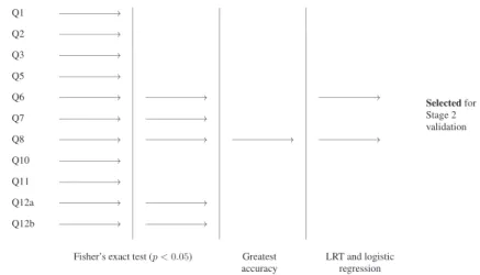
A schematic of the stage 1 selection process for breast cancer is given in Figure 1. Question 8 was the significant question with the highest balanced accuracy and was selected for further validation in stage 2. Question 6 was also selected on the basis of a likelihood ratio test.
Through its use of a two-stage design and a complex interim selection rule, the development of the brief FHQ has clear parallels to a biomarker discovery and validation study. Therefore, it inherits many of the same issues of bias and type I error inflation. In the next section, we describe how to derive efficient
Figure 1.Schematic of the stage 1 selection process for identifying sufficiently predictive questions for breast
cancer.
unbiased point estimates and confidence intervals under general selection rules, for which the FHQ study is a special case.
3. General framework for the uniformly minimum variance conditionally
unbiased estimator
3.1. Model description
Suppose there areKcandidate binary classifiers, each taking values in{0,1}. For example, this could correspond to a set ofKcandidate diagnostic biomarkers or a questionnaire withK‘yes’/‘no’ questions. The aim is to select the classifier that performs ‘best’ (as defined below), subject to passing a ‘fixed’ threshold and then to estimate its sensitivity. To do so, we perform a two-stage validation study.
In the first stage, each classifieriis tested on a population that containsn1iknown case subjects. These could be disease cases or those that have been classified as a case by some gold standard test. Ideally, the classifiers could be all tested on the same population; hence, then1i would all be equal. However, commonly, the number of case subjects will vary between the classifiers. This could be because of missing data or because the classifier is not applicable to all subjects (e.g. gender-specific questions).
LetXidenote the number of true positives for classifieri. Hence, we assume that we haveKindependent binomial variablesXi ∼Bin(n1i,si)fori =1,…,K, wheresiis the truesensitivityfor theith classifier and where sensitivity is defined as Prob(positive test∣subject diseased).
Each classifier has an associated fixed threshold that the number of true positives must pass in order to be considered further in stage 1. That is, for eachi∈ {1,…,K}there is a fixed cut-offci, and we require
Xi ⩾ ci or else classifieriis dropped for ‘futility’. For example, if there already exists a classifier with known sensitivityc̄, then we might setci =cn̄ 1i. If all the classifiers fail to pass their respective fixed thresholds, then the whole study is terminated early.
Suppose thatL>0 classifiers pass their fixed threshold. LetX∗
1,X
∗
2,…,X
∗
Ldenote the number of true
positives, where the relabelling preserves the original ordering of the labels (this is important for breaking ties). TheLclassifiers are then ranked from ‘best’ to ‘worst’ using a pre-specified functionr(X∗
i;𝝀i
) , where the𝝀iare constants associated with classifieri.
Thus, classifieri is ranked above classifierjif r(X∗
i;𝝀i ) > r ( X∗ j;𝝀j ) . If there is a tie,r(X∗ i;𝝀i ) = r ( X∗ j;𝝀j )
, we choose the classifier with the smallest index. This allows us to rank the classifiers in a prioriorder of importance. For instance, we might pre-rank the classifiers on the basis of evidence from previous studies, biological plausibility or simply the cost of measurement. A fully Bayesian approach is also possible, where classifiers are ranked using the posterior distribution of thesi, given the specification of suitable priors. Note that the method used for breaking ties is important. For example, Tappin [18] showed that if ties are broken by randomisation, then, in fact, no UMVCUE exists.
We also requirer(X∗
i;𝝀i
)
to induce the following inequalities on theX∗
i: r(Xi∗;𝝀i)⩾r ( X∗j;𝝀j ) ⇒X∗i ⩾d ( Xj∗;𝝀i,𝝀j ) fori,j∈ {1,…,L}, i≠j whered ( Xj∗;𝝀i,𝝀j )
is a function that only depends onXj∗,𝝀i,𝝀jand not onX∗i. Hence, there is equality if and only if there is a tie in the rankings. Note thatr(X∗
i;𝝀i
)
need not to be explicitly defined by the study organisers, as complex selection rules can be reverse engineered to conform to this set up, as we show for the FHQ study.
As an example of the above formulation, consider ranking the classifiers by their estimated sensitivities and, hence,𝝀i=n1iandr(X∗
i
)
=X∗
i∕n1i. This induces the following inequality: r(Xi∗;n1i)⩾r ( Xj∗;n1j ) ⇒X∗i ⩾d ( Xj∗;n1i,n1j ) =n1iXj∗∕n1j.
At the end of stage 1, the classifier with the highest ranking (that has passed its fixed threshold) is then selected for further validation in stage 2. LetMbe the index of this chosen classifier. In the second stage, the selected classifier from stage 1 is tested on a population containingn2 additional cases, wheren2is a constant that does not depend onX∗
M. LetYdenote the number of true positives in thesen2additional
observations. Note thatY∼Bin(n2,sM), independently ofX∗
M.
After the end of the study, we estimate the sensitivitysMof the selected classifier. The naïve estimator (MLE) forsMusing data from both stages is
̂
Sall∶= X ∗
M+Y n1M+n2.
This estimator is biased high, because it does not take into account the first stage selection procedures and soE[XM∗∕n1M|M]>sM.
An unbiased estimator Ŝ2 can easily be found by just using the stage 2 data, whereŜ2 ∶= Y∕n2. However, given the smaller sample size, then this estimator suffers from lower precision. Hence, we look for an unbiased estimator that utilises data from both stages.
3.2. Deriving the uniformly minimum variance conditionally unbiased estimator
In this section, we extend the arguments of Pepeet al.[5] and Tappin [18] to find the UMVCUE for the parameter of interestsM.
Let(i1,i2,…,iL)denote the vector of indices of the Lclassifiers Xi∗ after they have been ranked, with ties being decided by choosing the smaller index. Hence,M=i1is the index of the selected classifier. In what follows, we drop the * superscript for notational convenience. We drop the constants𝝀from the arguments of the functionsranddas well.
In Appendix A.1, we show that a complete and sufficient statistic for (s1,s2,…,sL) is Z = (
Z1,Z2,…,Z2L), where
Z1=Xi
1+Y,Z2=Xi2,…,ZL=XiL
ZL+1=i1,ZL+2=i2,…,Z2L=iL.
Let𝜓(i)denote the ranking of theithclassifier, andQthe event
{
𝜓(i1)=1, 𝜓(i2)=2,…, 𝜓(iL)=L;X1⩾c1,X2⩾c2,…,XL⩾cL}.
Then by the Lehmann–Scheffé theorem,Û ∶=E
(
Y n2
∣Z=z,Q
)
is the UMVCUE forsMunderQ. Now, following the idea of Pepeet al.[5], note that conditional onZ1 =Xi
1 +Y, the distribution of Yis hypergeometric:Y ∣ Z1 ∼Hyper(z1,n1M+n2−z1,n2), which can be re-expressed (for notational convenience) asY∣Z1 ∼Hyper(n2,n1M,z1). That is,
f(Y|Z1)= ( n2 y )( n1M z1−y ) ( n1M+n2 z1
) fory∈{max(0,z1−n1M),…,min(z1,n2)}.
The conditional density f(Y∣Z,Q) is essentially the same, except that the support of Y is further restricted byQ. There is the ranking condition inequalityr(Xi1)⩾r(Xi2)⇒Xi1 ⩾d(Xi2)and the fixed threshold conditionXi
1 ⩾ci1.
The precise way thatYis additionally restricted under(Z,Q)is given below. (1) y+xi
1 =z1
(a) Ifi1>i2 ⇒no tie in the ranking is possible
⇒xi1>d(xi2)⇒y<z1−d(z2) (b) Ifi1<i2 ⇒a tie is possible ⇒xi 1⩾d ( xi 2 ) ⇒y⩽z1−d(z2)
1421
(2) y+xi
1=z1andxi1 ⩾ci1 ⇒y⩽z1−ci1
The formula for the UMVCUE (assumingL>1) is then as follows.
̂ U=E ( Y n2 ∣Z=z,Q ) = ⎧ ⎪ ⎪ ⎪ ⎪ ⎪ ⎪ ⎨ ⎪ ⎪ ⎪ ⎪ ⎪ ⎪ ⎩ 1 n2 ∑ y∈A y ( n2 y )( n1M z1−y ) ∑ y∈A ( n2 y )( n1M z1−y ) ifi1 >i2andd(z2) ∈Z 1 n2 ∑ y∈B y ( n2 y )( n1M z1−y ) ∑ y∈B ( n2 y )( n1M z1−y ) otherwise (1) where
A={max(0,z1−n1M),…,min(z1−d(z2)−1,z1−⌈cM⌉,n2)} ∶conditions 1(a) and 2
B={max(0,z1−n1M),…,min(z1−⌈d(z2)⌉,z1−⌈cM⌉,n2)} ∶conditions 1(b) and 2 and⌈x⌉is the ceiling function acting onx.
Note that if the summation overygoes up ton2(so either max(A) =n2or max(B) =n2), then, in fact, ̂
U= z1
n1M+n2, which is just the usual MLEŜall. This makes it clear when the stage 1 selection exerts no
biasing effect at all.
IfL=1, then the dependence onZ2disappears, and we are left with the simpler formula below.
̂ U=E ( Y n2 ∣Z1=z1,Q ) = 1 n2 ∑ y∈A′ y ( n2 y )( n1M z1−y ) ∑ y∈A′ ( n2 y )( n1M z1−y ) whereA′={max(0,z 1−n1M ) ,…,min(z1−⌈cM⌉,n2)}.
3.3. Constructing confidence intervals
After calculating a point estimate forsMat the end of the study, it is natural to seek a confidence interval as well. In this section, we describe two schemes for generating confidence intervals.
3.3.1. Nonparametric bootstrap. Firstly, we adapt the nonparametric bootstrap procedure originally used by Pepeet al.[5]. Given trial dataZ, the procedure follows the resampling schema below.
(1) Resample the first stage data for the selected classifierM = i1 (with replacement). This gives a bootstrapped number of true positivesX(MB).
(2) IfXM(B)⩾cMandr ( XM(B) ) ⩾r(Xi 2 ) ,
(a) Resample the second stage data (with replacement), giving a bootstrapped number of true positivesY(B).
(b) Calculate the UMVCUEÛ(B)from equation (1), usingX(B)
M ,Y
(B)and the original observed valueXi
2.
These steps are then repeated for a large value ofB, so that there are enough sampled values ofÛ(B)to accurately assess its sampling distribution. The𝛼∕2 and(1−𝛼∕2)empirical quantiles are then used as the(1−𝛼)%confidence interval. Bootstrapped confidence intervals for the naïve estimatorsŜ2 andŜall
are also immediately available following this procedure.
3.3.2. Sill–Sampson approach. Alternatively, we can adapt the approach used by Sill and Sampson [16], who foundexactlikelihood-based confidence intervals forsMin the context of two-stage adaptive clinical trial. The derivation is similar to that in the work of Sill and Sampson [16], but we remove the control arm and also additionally allow for early stopping for futility and unequal first stage sample sizes. See Appendix A.2 for further details.
Defining X−1 ∶= (Xi
2,…,XiL
)
, then the conditional distribution used to find the confidence intervals is fQ(Z1|X−1)=𝜇−1[sM∕(1−sM)]Z1 ∑ XM∈D ( n1M XM )( n2 Z1−XM ) where 𝜇∶= n1M∑+n2 T=b [ sM∕(1−sM)]T ∑ XM∈D ( n1M XM )( n2 T−XM )
is the normalising constant and
D= { { max(d(Xi 2 ) +1,Z1−n2,⌈cM⌉,0),…,min(Z1,n1M)} ifi1 >i2andd(Xi 2 ) ∈Z { max(⌈d(Xi 2 )⌉ ,Z1−n2,⌈cM⌉,0),…,min(Z1,n1M)} otherwise b= { max(d(Xi 2 ) +1,⌈cM⌉,0) ifi1>i2andd(Xi 2 ) ∈Z max(⌈d(Xi 2 )⌉ ,⌈cM⌉,0) otherwise.
Suppose we observeZ1=Zobs. To construct the(1−𝛼)%confidence interval forsM, use the following functions: p1(sM)∶= Zobs ∑ Z1=b fQ(Z1|sM,X−1) and p2(sM)∶= n1M∑+n2 Z1=Zobs fQ(Z1|sM,X−1).
Bounds for a two-sided(1−𝛼)%confidence interval[Δ1,Δ2]can then be found by solving the equations
p2(Δ1)=𝛼1andp1(Δ2)=𝛼2respectively, where𝛼1+𝛼2=𝛼.
The original Sill–Sampson approach sets𝛼1=𝛼2=𝛼∕2, but this does not (in general) give the shortest confidence interval. We also experimented with choosing𝛼1and𝛼2to minimise the confidence interval length, which we refer to as ‘optimised’ Sill–Sampson confidence intervals.
3.3.3. Clopper–Pearson approach. In order to see how the Sill–Sampson approach compares with
using confidence intervals for the MLE, we use the well-known Clopper-Pearson method [20]. This uses the likelihood of the usual MLE to construct exact confidence intervals. Hence, the Sill–Sampson and Clopper–Pearson approaches are both likelihood based, but only the first takes into account the selection rules.
The Clopper–Pearson approach is as follows. Suppose we observeZ1 = Zobs. Then to construct the (1−𝛼)%confidence interval forsM, use the following functions:
p1(sM)∶= n1M∑+n2 Z1=Zobs ( n1M+n2 Z1 ) sZ1 M ( 1−sM)n1M+n2−Z1 and p2(sM)∶= Zobs ∑ Z1=0 ( n1M+n2 Z1 ) sZ1 M ( 1−sM)n1M+n2−Z1 .
1423
Bounds for a two-sided(1−𝛼)%confidence interval[Δ1,Δ2]can then be found by solving the equations
p2(Δ1)=𝛼∕2 andp1(Δ2)=𝛼∕2 respectively.
4. Simulation studies
We now perform a simulation study using a typical trial design. Consider a two-stage trial conducted onK
potential diagnostic biomarkers, where the interest is in finding the biomarker with the highest sensitivity. In stage 1, theithbiomarker is tested on a population that containsn
1iknown case subjects, where then1i
are not necessarily identical.
Suppose there already exists a biomarker with known sensitivityc̄ = 0.70. Hence, the fixed cut-off for biomarkeriis set toci =0.70n1i. The biomarkers that satisfyXi ⩾ciare then ranked by sensitivity, givingr(Xi)=Xi∕n1iandd(Xj)=n1iXj∕n1j. Finally, the selected biomarker (with labelM=i1) is taken forward to stage 2, where it is tested on an additional population withn2 =50 case subjects.
4.1. Point estimation
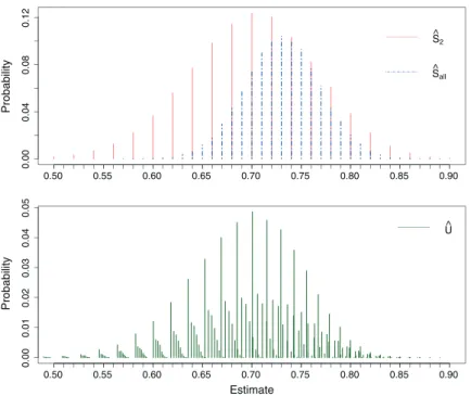
To start with, consider a simple simulation with K = 3 biomarkers with equal true sensitivities
S = (0.70,0.70,0.70). Each biomarker is tested on the same population of 50 case subjects, giving
n1 = (50,50,50) and c = 0.70n1 = (35,35,35). Figure 2 gives the probability mass functions of
100,000 realisations of the three estimatorsŜall, ̂S2 andÛ. Note the slight negative skew evident in the distribution ofÛ. The empirical biases and MSEs were (0.0308, -0.0001, -0.0001) and (0.0024, 0.0042, 0.0033) respectively.
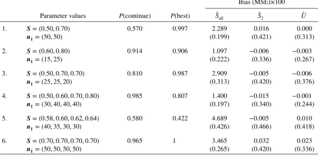
Table I shows the bias and MSE of the estimators for a range of further parameter values forSand
n1, where n2 = 50 and c = 0.70n1 as before. P(continue) gives the probability that the whole trial continues to the validation stage, whileP(best) is the probability that the biomarker with the highest (or joint-highest) sensitivity is selected for validation in stage 2, conditional on the trial actually continuing to the validation stage.
The MLEŜallis biased high, and this bias is most pronounced for larger values ofKand when the true sensitivities are similar. Note thatŜallis still biased even when the probability of continuing to stage 2 is close to 100% (e.g. scenario 6). This indicates two sources of bias: the bias due to early stopping and
0.00 0.04 0.08 0.12 Probability 0.50 0.55 0.60 0.65 0.70 0.75 0.80 0.85 0.90 0.00 0.01 0.02 0.03 0.04 0.05 Estimate Probability 0.50 0.55 0.60 0.65 0.70 0.75 0.80 0.85 0.90
Figure 2.Probability mass functions of the estimators forS= (0.70,0.70,0.70),n1= (50,50,50),c=0.70n1=
(35,35,35)andn2=50. Each mass function is based on 100,000 simulations.
Table I. Simulation results withn2=50 andc=0.70n1. The mean bias and MSE shown are 100 times the actual estimates. There were 100,000 simulations for each set of parameter values.
Bias (MSE)×100 Parameter values P(continue) P(best) Ŝall Ŝ2 Û 1. S= (0.50,0.70) 0.570 0.997 2.289 0.016 0.000 n1= (50,50) (0.199) (0.421) (0.313) 2. S= (0.60,0.80) 0.914 0.906 1.097 −0.006 −0.003 n1= (15,25) (0.222) (0.336) (0.267) 3. S= (0.50,0.70,0.70) 0.810 0.987 2.909 −0.005 −0.006 n1= (25,25,20) (0.313) (0.420) (0.376) 4. S= (0.50,0.60,0.70,0.80) 0.985 0.807 1.400 −0.015 −0.001 n1= (30,40,40,40) (0.197) (0.340) (0.244) 5. S= (0.58,0.60,0.62,0.64) 0.580 0.422 4.689 −0.005 0.010 n1= (40,35,30,30) (0.426) (0.466) (0.418) 6. S= (0.70,0.70,0.70,0.70) 0.965 1 3.465 0.032 0.023 n1= (50,50,50,50) (0.265) (0.420) (0.336)
the bias due to selecting the ‘best’ classifier from a set of candidates. The first source of bias would be expected to disappear when the probability of continuing to stage 2 is 100% but not the second.
The UMVCUEÛ is unbiased as expected, and it also has a lower MSE than the unbiased estimator ̂
S2 that only uses the stage 2 data. Indeed, there was a reduction of MSE ranging from 10% (for scenario 5) to 28% (for scenario 1). However,Û generally has a greater MSE thanŜall, by up to 57% (for scenario 1). This is not always the case – for scenario 5, the large bias ofŜall leads to a slightly greater MSE.
4.2. Interval estimation
We also consider the coverage of the confidence intervals constructed using the two procedures in Section 3.3, with𝛼=0.05. Table II shows the resulting mean coverage and confidence interval width for the scenarios in Table I.
The coverage for the MLEŜallcalculated using the nonparametric bootstrap is substantially lower than the nominal 95%, with values as low as 73% (for scenario 6). In contrast, the bootstrap coverage of the UMVCUEÛ is much closer to the nominal, hovering around 94% for all the scenarios. The bootstrapped confidence interval widths are greater forÛ than forŜall, with an increase ranging from 16% (for scenario 2) up to 51% (for scenario 7).
Using exact (likelihood-based) approaches give better coverage for both the MLE and UMVCUE, at the cost of slightly wider confidence intervals. For the MLE, the Clopper–Pearson approach gives conser-vative coverage for the majority of the scenarios, except for the last two sets of parameter values where the coverage was less than the nominal 95%. In contrast, the Sill–Sampson approach gives conservative confidence intervals for all the parameter values considered. This results in an increase in confidence interval width ranging from 11% (for scenario 2) up to 31% (for scenario 7).
Using optimised Sill–Sampson confidence intervals gives a slight reduction in width and coverage, although the latter is still above 95% in all the scenarios. However, this comes at a much greater computa-tional cost when simulating a large number of trials. Hence, we do not consider optimised Sill–Sampson confidence intervals any further in this research article.
4.3. Hypothesis testing
Consider now testing the hypothesisH0∶sM ⩽s∗versusH1 ∶sM>s∗, using exact 95% one-sided con-fidence intervals. We compare using Clopper–Pearson concon-fidence intervals forŜallwith the Sill–Sampson approach, whereH0is rejected ifs∗is less than the lower bound of the confidence interval. For a given set of true sensitivitiesS, letS0 ={s∈S∶s⩽s∗}. Then we define the conditional type I error rate as
T a ble II. Confidence interv al simulation results with 10,000 simulated trials for each set o f p arameter v alues. A s b efore, n2 =5 0a n d c = 0 . 70 n1 . T he number o f boot-strapped samples p er simulation w as set to B = 10,000. F o r comparison purposes, v alues for the optimised Sill–Sampson confidence interv als are sho wn in italics – note that only 1000 simulated trials w ere u sed h ere due to the computational cost. ̂Sall Sill–Sampson ̂U NP bootstrap C lopper – Pearson N P bootstrap P a rameter v alues Co v erage CI width C o v erage CI width C o v erage CI width C o v erage CI width 1. S =( 0 . 50 , 0 . 70 ) 0.966 0.228 0.934 0.215 0.965 0.183 0.892 0.153 n1 =( 50 , 50 ) 0.956 0.227 2. S =( 0 . 60 , 0 . 80 ) 0.969 0.214 0.945 0.196 0.966 0.193 0.938 0.169 n1 =( 15 , 25 ) 0.950 0.211 3. S =( 0 . 70 , 0 . 70 , 0 . 70 ) 0.965 0.233 0.940 0.222 0.951 0.181 0.825 0.150 n1 =( 50 , 50 , 50 ) 0.957 0.232 4. S =( 0 . 50 , 0 . 70 , 0 . 70 ) 0.968 0.249 0.941 0.236 0.949 0.219 0.885 0.188 n1 =( 25 , 25 , 20 ) 0.962 0.248 5. S =( 0 . 50 , 0 . 60 , 0 . 70 , 0 . 80 ) 0.965 0.204 0.943 0.188 0.958 0.174 0.904 0.150 n1 =( 30 , 40 , 40 , 40 ) 0.964 0.201 6. S =( 0 . 58 , 0 . 60 , 0 . 62 , 0 . 64 ) 0.961 0.262 0.943 0.256 0.913 0.212 0.731 0.180 n1 =( 40 , 35 , 30 , 30 ) 0.958 0.262 7. S =( 0 . 70 , 0 . 70 , 0 . 70 , 0 . 70 ) 0.961 0.236 0.937 0.225 0.942 0.180 0.793 0.149 n1 =( 50 , 50 , 50 , 50 ) 0.955 0.235
1426
𝛼 = P(rejectH0|sM∈S0,Q). The unconditional type I error rate is defined asP(rejectH0,sM∈S0), where there is no conditioning on continuing to stage 2.
Similarly, the conditional power of the test is defined asP(rejectH0|sM∈S∖S0,Q). The unconditional power isP(rejectH0,sM∈S∖S0), with no conditioning on continuing to stage 2.
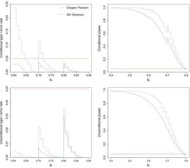
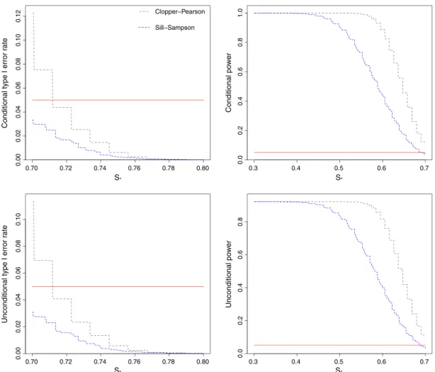
Figure 3 shows the conditional and unconditional type I error rates and powers when the sensitivities are constrained to the setS = (0.50,0.60,0.70,0.80), with stage 1 sample sizesn1 = (30,40,40,40). Using the Clopper–Pearson confidence intervals forŜallcan give highly inflated conditional type I error rates (as high as 24%), particularly for values ofs∗that are just above 0.60 or 0.70.
In contrast, using the Sill–Sampson approach guarantees that the conditional type I error rate will be less than 5% for all values ofs∗. This comes at the cost of lower power, both conditionally and uncondi-tionally. Note that while using exact confidence intervals for the MLE does not control the type I error conditionally, it does control it unconditionally sinceP(sM ∈S0)is low whens∗<0.70.
Figure 4 shows the conditional and unconditional type I error rates and powers for the scenario
S= (0.70,0.70,0.70)andn1 = (50,50,50). This time, using the confidence intervals forŜallgives inflated
type I error rates both conditionally and unconditionally. Even unconditionally, the type I error rate can be as high as 11%. In contrast, the Sill–Sampson approach again guarantees that the type I error rate will be less than the nominal 5%. However, this is at the cost of a substantial loss of power compared with using the MLE.
0.60 0.65 0.70 0.75 0.80 0.85 0.90 0.00 0.05 0.10 0.15 0.20 0.25 S* S* S* S*
Conditional type I error r
ate Clopper−Pearson Sill−Sampson 0.4 0.5 0.6 0.7 0.8 0.0 0.2 0.4 0.6 0.8 1.0 Conditional po w e r 0.60 0.65 0.70 0.75 0.80 0.85 0.90 0.00 0.01 0.02 0.03 0.04 0.05
Unconditional type I error r
a te 0.4 0.5 0.6 0.7 0.8 0.0 0.2 0.4 0.6 0.8 1.0 Unconditional po w e r
Figure 3.Conditional and unconditional type I error rates and power for testing the hypothesisH0 ∶ sM ⩽ s∗
versusH1∶sM>s∗, using exact 95% one-sided confidence intervals. The true sensitivities are constrained to the
setS= (0.50,0.60,0.70,0.80), with stage 1 sample sizesn1= (30,40,40,40). Plots show the results from 10,000 simulated sets of trial data. The horizontal line shows the nominal 5% level.
0.70 0.72 0.74 0.76 0.78 0.80 0.00 0.02 0.04 0.06 0.08 0.10 0.12 S* S* S* S*
Conditional type I error r
ate Clopper−Pearson Sill−Sampson 0.3 0.4 0.5 0.6 0.7 0.0 0.2 0.4 0.6 0.8 1.0 Conditional po w e r 0.70 0.72 0.74 0.76 0.78 0.80 0.00 0.02 0.04 0.06 0.08 0.10
Unconditional type I error r
a te 0.3 0.4 0.5 0.6 0.7 0.0 0.2 0.4 0.6 0.8 Unconditional po w e r
Figure 4.Conditional and unconditional type I error rates and power for testing the hypothesisH0 ∶ sM ⩽ s∗
versusH1 ∶ sM > s∗, using exact 95% one-sided confidence intervals. The true sensitivities are constrained to the setS = (0.70,0.70,0.70), with stage 1 sample sizesn1 = (50,50,50). Plots show the results from 10,000
simulated sets of trial data. The horizontal line shows the nominal 5% level.
5. Application to the family history questionnaire study
In this section, we return to the motivating example of the two-stage FHQ study by Walteret al.[19]. Although a𝜒2-test for concordance was carried out before pooling data from the two stages, a natural
question to ask is whether any bias was induced into the results by the stage 1 selection rules. Using the framework for bias adjusted inference outlined in Section 3, we calculate the UMVCUE and exact confidence intervals for the sensitivities of the selected questions.
5.1. Model description for the family history questionnaire
We use a slightly simplified version of the study design formulated in Section 3.1. Note that this model does not consider combinations of questions; hence, steps 3 and 4 in stage 1 are ignored. In the discussion, we comment on how the approach could potentially be extended to consider combinations of questions. In what follows, the focus is on estimating the sensitivity of the selected questions. The model for estimating the specificity, or other measures of diagnostic performance, will be very similar.
In the first stage,K questions are assessed on a case-control population, with the results for theith
question available onn1icases andm1icontrols. LetXidenote the number of true positives (TP) for the
ith question (i =1,…,K). That is, the total number of ‘yes’ responses from the case population. Then
theXi are assumed to follow independent binomial populations:Xi ∼ Bin(n1i,si), wheresi denotes the true sensitivity of questioni. In Section 5.3.2 we explore the performance of the method when this independence assumption in violated, as was the case (to a very limited extent) with the FHQ data.
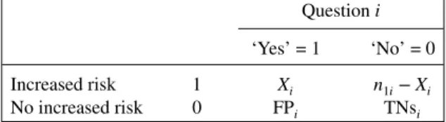
Table III. Contingency table for Fisher’s exact test. Questioni ‘Yes’ = 1 ‘No’ = 0 Increased risk 1 Xi n1i−Xi
No increased risk 0 FPi TNsi
It is worth noting that when analysing the sensitivity of the selected questions, we are explicitly condi-tioning on the specificity results (i.e. the number of false positives and true negatives) in addition to what was specified in Section 3.2. We use this fact for both of the selection procedures: Fisher’s exact test and ranking by balanced accuracy.
5.1.1. Fisher’s exact test cut-off. Firstly, Fisher’s exact test is applied to the contingency table given in Table III where FPi= number of false positives and TNi= number of true negatives for questioni. As the focus is in estimating the sensitivity and we are conditioning on the observed specificity results from the trial, then the values of FPiand TNiare considered fixed for eachi.
The aim is to find the threshold that Xi must pass in order for Fisher’s exact test to give a p-value
pi<0.05. That is, the value ofcisuch thatXi⩾ci⇒pi<0.05. Because the FPiand TNiare fixed, then we can do so by simply settingcias the smallest value in{0,1,…,n1i}such thatpi<0.05 for allXi⩾ci. Note that the conditioning on the observed number of false positives and true negatives is important. Indeed, another way of finding the Fisher’s exact test threshold for theXiwould be to only consider the row and column totals as fixed, hence, allowing FPiand TNi to vary also. However, this would induce dependence between theXiand theci, which would invalidate the derived form of the UMVCUE.
Although a two-sided Fisher’s exact test was used in a study, we did not have to consider departures towards the other extreme – i.e. values ofXi ≪ bi that gave pi < 0.05. This was because all of the significant questions in the study actually passed the upper thresholdci. In addition, we would not be interested in a question that had especially low values ofXi, because this would imply a low sensitivity. The balanced accuracy ranking (see the succeeding paragraphs) should rule out such questions being carried forward to stage 2.
In summary, for eachi∈ {1,…,K}, there is an associated fixed thresholdci. IfXi⩾cithen Fisher’s exact test will give ap-value<0.05; thus,Xiwill be considered further in the balanced accuracy ranking.
SupposeL>0 questions are identified as significant. LetX∗
i (i=1,…,L) denote the number of true
positives, where the relabelling preserves the order of the original labelling.
5.1.2. Balanced accuracy ranking. The significant question with the greatest balanced accuracy is now selected. If there is a tie (which did not occur in the study data), we assume that the question with the smallest index would be chosen.
Now, suppose questionihas a greater balanced accuracy than questionj. This implies the following inequality onX∗
i andX
∗
j:
Accuracyi⩾Accuracyj
⇒(Sensitivityi+Specificityi)⩾(Sensitivityj+Specificityj)
⇒ X ∗ i n1i +Spi⩾ X∗j n1j +Spj ⇒Xi∗⩾n1i(Spj−Spi) + n1i n1jX ∗ j (2) where Spi=Specificityi∶= TNi TNi+FPi .
Let(i1,i2,…,iL) denote the vector of indices of theXi∗ after they have been ordered by balanced accuracy, and letM=i1. Then from equation (2) the following inequality holds:
X∗M⩾nM(Spi 2−SpM ) +n1M n1,i 2 X∗i 2. (3)
1429
In the second stage, we test the selected questionMfrom stage 1 onn2additional cases andm2 addi-tional controls. LetYdenote the number of true positives recorded in stage 2. Note thatY∼Bin(n2,sM), and is independent ofXM.
5.2. The uniformly minimum variance conditionally unbiased estimator
To find the UMVCUE for the sensitivitysMof the selected question (after the end of stage 2), we use equation (1), where d(Z2)= n1MZ2 n1,i 2 +n1M(SpM−Spi 2 ) .
Equation (1) holds when the number of significant questionsLsatisfiesL>1, which is what occurred in this study for all of the diseases considered.
5.3. Results
We now apply our results to the trial data from the FHQ study, first repeating the analysis carried out in the work of Walteret al. [19]. Fisher’s exact test indicated that an increased risk of diabetes was associated with questions 1 and 3 (p = 0.004 andp < 0.001). For IHD, questions 1, 2, 3 and 8 were significant (p=0.013,p<0.001,p=0.018 andp=0.048). For breast cancer (females only), there was a significant association for questions 6, 7, 8, 12a and 12b (p<0.001,p<0.001,p<0.001,p<0.001 andp = 0.002). Finally, increased risk of colorectal cancer was associated with questions 10 and 11 (p<0.001 for both).
Table IV shows the sensitivities, Fisher’s exact test thresholds (FT) and balanced accuracies for each question. The questions that passed the Fisher threshold are shown in bold, with the ultimately selected question also boxed. If the significant question with the highest balanced accuracy is chosen, then ques-tion 3 is selected for diabetes, quesques-tion 2 for IHD, quesques-tion 8 for breast cancer and quesques-tion 10 for colorectal cancer.
5.3.1. Uniformly minimum variance conditionally unbiased estimator for the selected questions. Using
the data from stages 1 and 2, we now calculate the value of the UMVCUEÛ for the sensitivity of the selected question for each condition, and compare it with the various naïve estimators of the sensitivity (̂S1, ̂S2, ̂Sall).Ŝ2andŜallare defined as before, whileŜ1 ∶=XM∕n1Mis the estimated sensitivity just using the stage 1 data.
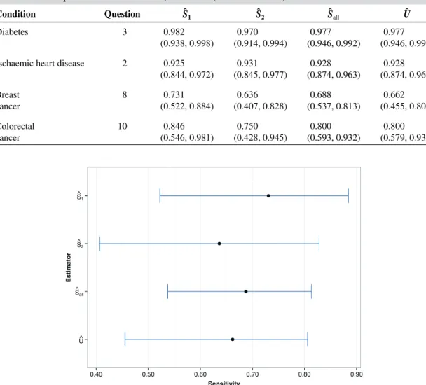
Table V gives the values of the estimators for each disease, along with exact (likelihood-based) two-sided 95% confidence intervals. For(Ŝ1, ̂S2, ̂Sall), Clopper–Pearson confidence intervals are used, while the Sill–Sampson confidence interval is shown forÛ.
For diabetes, IHD and colorectal cancer, the UMVCUE isidenticalto the MLEŜallthat uses data from both stages. This is a consequence of the formula forÛ as described earlier. In addition, the Sill–Sampson confidence intervals for diabetes and IHD are virtually identical to the Clopper–Pearson intervals forŜall. This is an attractive feature: the approach is able to identify when selection bias isnotan issue.
However, for breast cancer, the UMVCUE is smaller thanŜall. Looking at the individual estimates for the stagesŜ1andŜ2, there is an especially large relative drop from 0.731 to 0.636 between stages 1 and 2, which supports the idea that the stage 1 data was biased high by the selection criteria. Figure 5 gives a graphical representation of the breast cancer data.
If we follow Walteret al.[19] and use Pearson’s𝜒2-test to compare the sensitivity between the two stages, thep-values are 0.873, 1.000, 0.696 and 0.920 for diabetes, IHD, breast cancer and colorectal can-cer, respectively. It is interesting to note that thep-value for breast cancer is substantially lower than those for the other diseases, although it is still far above 0.05. This suggests that the𝜒2-test is too conservative
as a tool for detecting bias in the stage 1 data.
Indeed, for breast cancer, suppose we assume that the stage 1 data as well as the total number of cases in stage 2 are fixed. Then the number of true positives in stage 2 would have to be less than or equal to 8 (i.e. a sensitivity less than 0.363) in order for the𝜒2-test to reject the null hypothesis.
5.3.2. Correlation. Finally, we consider the effect of correlation on the sensitivity estimates for the FHQ data. Recall that the data were assumed to be drawn from independent populations. However, in the FHQ study, each participant answered multiple questions. It sometimes happens that the answer to
Ta b le IV . Stage 1 sensiti vities, Fisher’ s ex act test thresholds (FT) and b alanced accuracies for each condition. Questions passing the F T are sho w n in bold, with the selected question also box ed.
1431
Table V. Uniformly minimum variance conditionally unbiased estimators (UMVCUE) and naïve estimators for the selected questions for each disease, with exact (likelihood-based) 95% confidence intervals.
Condition Question Ŝ1 Ŝ2 Ŝall Û
Diabetes 3 0.982 0.970 0.977 0.977
(0.938, 0.998) (0.914, 0.994) (0.946, 0.992) (0.946, 0.992) Ischaemic heart disease 2 0.925 0.931 0.928 0.928
(0.844, 0.972) (0.845, 0.977) (0.874, 0.963) (0.874, 0.963) Breast 8 0.731 0.636 0.688 0.662 cancer (0.522, 0.884) (0.407, 0.828) (0.537, 0.813) (0.455, 0.806) Colorectal 10 0.846 0.750 0.800 0.800 cancer (0.546, 0.981) (0.428, 0.945) (0.593, 0.932) (0.579, 0.932) U^ S^all S^2 S^1 0.40 0.50 0.60 0.70 0.80 0.90 Sensitivity Estimator
Figure 5.Plot of point estimates and exact (likelihood-based) 95% confidence intervals for the breast cancer data.
Table VI. Correlation matrix for all of the stage 1 data in the family history questionnaire study, using
pairwise-complete responses. Q1 Q2 Q3 Q5 Q6 Q7 Q8 Q10 Q11 Q12a Q12b Q1 1 0.142 0.121 0.051 0.072 0.028 0.096 0.047 0.086 0.049 0.062 Q2 0.142 1 0.101 0.090 0.056 0.033 0.062 0.006 0.050 0.002 0.063 Q3 0.121 0.101 1 −0.003 0.067 0.027 0.013 0.005 0.069 0.022 0.029 Q5 0.051 0.090 −0.003 1 0.006 0.016 0.014 −0.049 −0.014 0.121 0.012 Q6 0.072 0.056 0.067 0.006 1 0.005 0.018 0.045 −0.002 0.085 0.096 Q7 0.028 0.033 0.027 0.016 0.005 1 0.282 0.004 −0.007 0.116 0.124 Q8 0.096 0.062 0.013 0.014 0.018 0.282 1 −0.023 0.056 0.240 0.112 Q10 0.047 0.006 0.005 −0.049 0.045 0.004 −0.023 1 0.193 0.084 0.112 Q11 0.086 0.050 0.069 −0.014 −0.002 −0.007 0.056 0.193 1 0.187 0.121 Q12a 0.049 0.002 0.022 0.121 0.085 0.116 0.240 0.084 0.187 1 0.395 Q12b 0.062 0.063 0.029 0.012 0.096 0.124 0.112 0.112 0.121 0.395 1
one questions should (logically at least) determine the answer to another question as well. For example, answering ‘yes’ to question 12b should mean that the answer to question 12a will also be ‘yes’. For these two reasons, we might expect there to be some correlation between the sensitivity estimates for different questions. The correlation matrix (using pairwise-complete responses) for all of the stage 1 data is displayed in Table VI.
Reassuringly, the correlations between all of the questions appears to be rather small, with a mean (absolute) pairwise correlation of just 0.07. The maximum correlation coefficient was 0.395, for the pair (Q12a, Q12b), which is explained by the aforementioned reason.
Nevertheless, we simulated FHQ-like data with the above correlation structure, using a modified version of the R packagebindata[21]. The true sensitivities were assumed equal to the estimated stage 1 sensitivities, with 50,000 simulated data sets for each condition. For breast cancer the UMVCUE had a mean bias of -0.0082, which is less than 32% of the observed correction to the MLE for the actual FHQ data. For the other diseases there was no appreciable bias.
6. Discussion
In this research article, we present a framework for conditional estimation for a general two-stage trial design with binary classifiers. By allowing for generalised selection rules and arbitrary futility thresholds, our estimation strategy can be applied to a wide range of two-stage validation study designs. In particular, complex ranking criteria can be reverse engineered to fit within our framework.
We showed that using the usual MLE can lead to substantial conditional bias, especially when there are many candidate classifiers under consideration with similar true sensitivities. In contrast, the UMVCUE is indeed unbiased but often at the expense of a larger MSE. However, there are still large savings in efficiency when compared with just using the unbiased stage 2 data.
The usual MLE also can suffer from incorrect confidence interval coverage and inflated type I error rates for hypothesis testing, both conditionally and unconditionally. These issues can be avoided by using the Sill–Sampson approach to find exact confidence intervals, although this comes at the cost of reduced power. Although this approach is somewhat conservative, when presenting the results of a trial to a reg-ulatory authority, any inflation in the type I error rate above the advertised level is likely to be deemed unacceptable [16].
The application of our inferential technique to the FHQ data demonstrated how the UMVCUE can identify whether selection bias is an issue. Point estimates for the selected questions using the UMVCUE and the MLE were identical for three of the conditions, with virtually identical confidence intervals as well. However, for breast cancer, the UMVCUE was able to identify and correct for the bias induced in the MLE. We also found that with the correlation structure present in the FHQ data, these results were not significantly affected by the minor violations of the independence assumption.
Our focus in this research article was in deriving unbiased estimators for the true sensitivity of the chosen classifier. However, by relaxing the unbiasedness condition slightly, it may be possible to achieve a lower MSE. One approach we tried was to usemedian unbiased estimates, as described by Jovic and Whitehead [22]. Briefly, using the distribution functionsp1(sM)andp2(sM)defined for the Sill–Sampson approach, the (approximate) median unbiased estimator is given by 1
2
(
Δ1+ Δ2), where
p2(Δ1)=0.5 andp1(Δ2)=0.5. However, we found that there was no gain over the UMVCUE in terms of MSE, and the estimator was indeed biased slightly low in its mean.
We only considered a design that selects and evaluates the performance of a single classifier. However, many studies (including the FHQ study)combinemultiple classifiers intorisk prediction models. Much further research is needed to explore conditional estimation for combinations of classifiers, especially given the wide variety of model selection and validation procedures present in the literature. For example, recent work by Koopmeinerset al.[23] describes the issue of testing and validating a panel of biomarkers. Accounting for correlation will clearly be essential here too.
One way to try and deal with correlated classifiers is to decorrelate the variables of interest, as described by Zuber and Strimmer [24] in the context of biomarker discovery and gene-ranking byt-scores. However, is not clear whether similar transformations can be applied to binary data without altering its distribution. A related issue would be to considerjointinference on the sensitivity and specificity. As mentioned in Section 5, by conditioning on the observed specificity results we treated the number of true negatives (and false positives) as fixed values. If we instead considered the number of true negatives as a binomial random variable (possibly correlated with the number of true positives), then further work would be needed to allow conditionally unbiased estimation. A complicating factor would be determining how the ranking criterion and ‘fixed’ thresholds change as the number of true positives and negatives are jointly varied.
Finally, another extension would be to consider inference trials with more than two stages. Bowden and Glimm [11] describe conditionally unbiased estimates for normally distributed outcomes with multiple stages of selection, and their approach could be extended to the binomial setting.
Appendix A
A.1. Proof of the completeness and sufficiency of Z
Here we prove the following theorems (originally theorems 2.1 and 3.1 in the work of Tappin [18]).
Theorem A.1
The statisticZ=(Z1,Z2,…,Z2L)is sufficient for(s1,s2,…,sL), where
Z1=XM+Y,Z2=Xi
2,…,ZL=XiL
ZL+1=i1,ZL+2=i2,…,Z2L=iL Proof
The joint distribution ofX,Yis as follows:
f(X,Y) = ( n1M XM ) sXM M ( 1−sM)n1M−XM ( n2 Y ) sYM(1−sM)n2−Y ×∏ j≠M ( n1j Xj ) sXj j ( 1−sj)n1j−Xj = [ sXM+Y M ( 1−sM)n1M+n2−(XM+Y)∏ j≠M sXj j ( 1−sj)n1j−Xj ] × [( n1M XM )( n2 Y ) ∏ j≠M ( n1j Xj )] .
Thus according to the factorisation criteria, the statisticZis sufficient for(s1,s2,…,sL).
Theorem A.2
When ties are broken by selecting the population with the smallest index, the sufficient statisticZis also complete.
Proof
Following Tappin [18] and Jung and Kim [25], we prove the result forL=2 classifiers, and note that the argument easily extends to arbitraryL>2.
For an arbitrary function g(⋅), defined on the range of Z, we will show that Es
[
g(z)] ≡ 0 for all
s =⇒ g(z)≡0. Without loss of generality, we assume thatd(z2)∈Z. Let
A1 ={Z∶z3 =1,⌈ci 2⌉⩽z2 ⩽n1i2,max ( 0,⌈cM⌉,d(z2))⩽z1⩽n1M+n2} A2 ={Z∶z3 =2,⌈ci 2⌉⩽z2 ⩽n1i2,max ( 0,⌈cM⌉,d(z2)+1)⩽z1 ⩽n1M+n2}. Note thatZ1 =XM,Z2 =Xi
2,Z3=M=i1andZ4=i2. BecauseZ1 =XM+Y, then the distribution of ( X,Z1)is given by f(X,Z1)= ( n1M XM )( n12 Z2 )( n2 Z1−XM ) sZ1 M ( 1−sM)n1M+n2−Z1 sZ2 2 ( 1−s2)n12−Z2
We can now find the distribution ofZby summing over the support ofXM:
f(Z) =𝜅(z)sZ1 M ( 1−sM)n1M+n2−Z1 sZ2 2 ( 1−s2)n12−Z2.