4-29-2008
Semiparametric Inferential Procedures for
Comparing Multivariate ROC Curves with
Interaction Terms
Liansheng Tang
Xiao-Hua Zhou
Suggested Citation
Tang, Liansheng and Zhou, Xiao-Hua, "Semiparametric Inferential Procedures for Comparing Multivariate ROC Curves with Interaction Terms" (April 2008).UW Biostatistics Working Paper Series.Working Paper 326.
Semiparametric Inferential Procedures for Comparing
Multivariate ROC Curves with Interaction Terms
Liansheng Tang1, Xiao-Hua Zhou2,3,∗
1George Mason University, 2University of Washington, 3 VA Puget Sound Health Care System
Abstract: Multivariate ROC curve models that include an interaction term be-tween biomarker type and false positive rate is important in comparative biomarker studies, because such interaction allows ROC curves of different biomarkers to cross each other. However, there has been limited work in drawing inference for comparing multivariate ROC curves, especially when the interaction terms are present. In this article we derive the asymptotic covariance of three estimators for multivariate ROC models. These covariance estimates have not been readily available in the literature, and bootstrap methods have to be used to obtain co-variance estimates. With the readily available co-variance estimates, we can easily perform hypothesis testing among ROC curves while bootstrap tests are not so easily performed. The asymptotic results are applied to compare ROC curves and their areas under ROC curves. Moreover, we derive simultaneous confidence bands for multivariate ROC curves. We evaluate and compare the finite sample performance of our asymptotic covariance estimators. We also discuss the ad-vantage of using our asymptotic results over bootstrap procedures. Finally, we illustrate our approach through a well-known pancreatic cancer study.
Key words and phrases: Diagnostic Accuracy, Simultaneous Confidence Band, Brownian Bridge Process.
1. Introduction
Research in early cancer detection involves developing diagnostic tools, such as a biomarker, to distinguish diseased patients from non-diseased patients. Biomarkers often yield continuous measurements. A popular tool to evaluate and compare the accuracy of biomarkers is a receiver operating characteristic (ROC) curve (Zhou et al., 2002), which is a plot of true positive rates vs false positive rates across all thresholds. Estimating a single binormal ROC curve of a continuous-scale biomarker has been well studied in the literature (Metz,
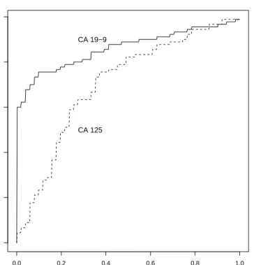
Herman and Shen, 1998; Cai and Moskowitz, 2004). However, inferential pro-cedures for comparing multivariate ROC curve models with interaction terms between biomarker type and false positive rates (FPRs) have not been well stud-ied, mainly because it is sometimes difficult to draw inferences in the presence of these interaction terms. However, such interactions are important because they allow ROC curves to cross each other. For example, Wieand et al. (1989) stud-ied pancreatic cancer biomarkers, CA 19-9 and CA 125, which were measured on 51 pancreatitis patients and 90 pancreatic cancer patients. The empirical ROC curves were generated from this data set and their plots are shown in Figure 1. It is clear that two ROC curves cross each other when FPR gets close to 1. This fact shows the existence of interaction terms between biomarker type and FPRs.
Insert Figure 1 here.
Metz, et al. (1984) proposed a maximum likelihood estimator (MLE) for estimating bivariate binormal models from ordinal data. But their method re-quires estimating correlation parameters, besides the location and scale param-eters in the marginal normal distributions. It would be more difficult to further extending their MLE method to more than two ROC curves when many more correlation parameters are to be estimated. As the number of biomarkers gets large, the MLE method becomes nonapplicable. For multiple independent ROC curves, Zhang (2004) and Zhang and Pepe (2005) proposed an intuitive least squares (LS) method, and Pepe (2000) presented an elegant generalized linear model (GLM) approach. Since it is complicated to derive the asymptotic results, the authors did not consider the large sample inference for the LS and GLM estimators with clustered data. Cai and Pepe (2002) considered an interesting semiparametric generalized estimating equation (GEE) method to allow an un-known baseline function when estimating ROC curves from correlated biomarker data. They derived asymptotic results for their estimators, but they did not con-sider how to compare multiple ROC curves from clustered data with the presence of interactions between biomarker type and FPRs.
In this article we adapt the LS method to clustered ROC curve data with the presence of interactions between biomarker type and FPRs. We derive explicit covariance structures between empirical ROC curves and use our results to derive
the asymptotic covariances of the LS estimator. We also adapt the GLM and GEE methods to this type of biomarker data and derive their asymptotic sand-wich covariance estimators. These covariances have not been readily available in the literature, and bootstrap methods have to be used to obtain covariance estimates. With the readily available variance estimates, we can easily perform hypothesis testing among ROC curves while bootstrap tests are not so easily performed. For example, if we want to test whether two ROC curves vary by a certain amount δ at a specified FPRu0, i.e., H0 :ROC1(u0)−ROC2(u0) = δ, it is not clear how to bootstrap from the null distribution, while it is straight-forward to perform such hypothesis tests using our asymptotic results and the delta method, which will be introduced in Section 4. We derive inferential proce-dures for comparing multivariate ROC curves that include the interaction terms, which have multivariate binormal ROC curves as a special case. In particular, we develop methods for comparing ROC curves and the areas under these ROC curves. We derive asymptotic simultaneous confidence bands for ROC curves. Such asymptotic results of simultaneous confidence bands of ROC curves are rarely studied. Instead, computer intensive methods are often employed to con-struct confidence bands (Cai and Pepe, 2002). Our confidence bands provide an easy-to-use tool to illustrate the sampling variability of the ROC curve estimates. In addition, we develop a method for comparing multiple ROC curves at some specified FPR.
This article is organized as follows. In Section 2 we adapt the LS methods to estimate multivariate ROC curves, and we also adapt GLM and a simplified GEE method. In Section 3 we derive the asymptotic results for the LS method when estimating multivariate ROC models. The asymptotic results are also derived for GLM and GEE methods. In Section 4 we apply the results to draw inference on comparing ROC curves and the areas under the ROC curves. In addition, asymptotic simultaneous confidence bands are derived for multivariate ROC curves. We carry out large scale simulation studies to evaluate and compare the finite sample performance of our covariance estimators of the LS, GLM and GEE methods. We also carry out simulation studies to evaluate the advantages of using asymptotic results over using bootstrap procedures. The simulation results are summarized in Section 5. A comparative pancreatic cancer diagnostic trial
serves as an illustrative example in Section 6, and some discussions are presented in Section 7.
2. Three estimators of multivariate ROC curves
In this section, we adapt the LS and GLM methods to clustered ROC data. We also give a simplified version of the GEE method for estimating multivari-ate ROC curves. Let X` = (X`,1, X`,2, ..., X`,m) denote measurements of the
`th biomarker on m diseased subjects, and Y`˜= (Y`,1˜ , Y`,2˜ , ..., Y`,n˜ ) denote mea-surements of the ˜`th biomarker on n healthy subjects, where `,`˜ = 1, ..., K. For the `th and ˜`th different biomarkers measured on the ith diseased subject,
i= 1, ..., m, the measurementsX`,iandX`,i˜ follow the bivariate survival function F`,`˜ with the marginal distributions F` and F`˜, respectively, and the measure-ments of thejth healthy subject,Y`,j andY`,j˜ withj= 1, ..., n, follow the bivari-ate survival functionG`,`˜with the marginal distributionsG`andG`˜, respectively. The ROC curve of the`th biomarker is then given byQ`(u) =F`(G−`1(u)),and its empirical form is Qe`(u) =Fb`(Gb`−1(u)), whereFb` and Gb` are empirical functions of F` and G`, respectively.
Let Zk be a dummy variable for the kth biomarker, k = 2, ..., K. The multivariate ROC curves are then given by the following expressions:
Q1(u) = g{θ10+θ11h(u)}, and Qk(u) = g[θ10+θ11h(u) + K X i=2 {θi0Zi+θi1Zih(u)}], (2.1)
for 0 < a ≤ u ≤ b < 1, where g is some specified link function and h is some specified baseline function. In the regression ROC modeling,θ10+θ11h(u) is the baseline function, usually denoted as h0(u). In this article we let this baseline function be a known function up to two unknown parameters,θ10 andθ10, as in Pepe (2000), Zhang (2004) and Zhang and Pepe (2005). The important compo-nents of the model (2.1) areθk1Zkh(u), which are the interaction terms between dummy variables indicating biomarker types and FPRs. Such interaction terms play an important role in estimating ROC curves especially when estimating the multivariate binormal ROC curves. With these terms, the model (2.1) includes the multivariate binormal ROC model as a special case, which is commonly used in the literature (Metz, et al., 1984). Specifically, let g be Φ, leth be Φ−1 and
let Zk be an indicator variable for the kth biomarker, the model (2.1) has the following expressions:
Q1(u) = Φ{θ10+θ11Φ−1(u)}
and Qk(u) = Φ{θ10+θ11Φ−1(u) +θk0+θk1Φ−1(u)}, (2.2) for k= 2, ..., K. When there is only one biomarker, the model (2.2) reduces to the commonly used binormal model (Zhou, et al., 2002).
Letu`= (u`,1,· · ·, u`,P`)T be some fixed partition points in the range of [a, b] on the `th empirical ROC curve. Here P` is arbitrarily chosen for the `th ROC curve where 0< a=u`,1 < u`,2 < ... < u`,P` =b <1. For example, if we choose
50 jump points for the 1st ROC curve, we can chooseu1 = (1/51,2/51, ...,50/51). Also, for simplicity, we denote L(u`) = (L(u`,1), L(u`,2), ..., L(u`,P`))T, where `= 1, ..., K, for any process or functionL.
Zhang (2004) and Zhang and Pepe (2005) proposed a least squares (LS) ap-proach to estimate multiple ROC curves. They letZk be the indicator variables for the kth biomarker. In the LS estimating procedure, the ROC curve corre-sponding to a reference biomarker is chosen as the reference ROC curve. For the
`th empirical ROC curve, the partition points, u` = (u`,1,· · · , u`,P`)T, are cho-sen within interval boundaries [a, b]. When we are interested in the entire ROC curve, a and b can be chosen to be close to 0 and 1, respectively. If a partial ROC curve is of interest,a andb can be chosen accordingly. By plugging in the empirical functions Fb` and Gb−`1, the `th empirical ROC curve is computed by
e
Q`(u`) =Fb`(Gb−`1(u`)). Denote Ye` =g−1(Qe`(u`)). We combine Ye1,Ye2, ...,YeK and get a linear regression equation as follows:
e
Y =M θ+², (2.3)
whereYe = (Ye1T, ...,YeKT)T is a (P`P`)×1 vector with its elementYe`=g−1(Qe`(u`)). The (P`P`)×(2K) design matrixM is given by:
M = M1 0 0 · · · 0 M2 M2∗ 0 · · · 0 M3 0 M3∗ · · · 0 .. . ... ... . .. ... MK 0 0 · · · M∗ K ,
with itsP`×2 submatrices M`= Ã 1 · · · 1 h(u`,1) · · · h(u`,P`) !T , and Mk∗= Ã Zk · · · Zk Zkh(u`,1) · · · Zkh(u`,P`) !T .
Also, the error term ² has a multivariate normal distribution given by ² ∼
N(0,Σ²). The detailed proof is given in in the on-line version of the paper at http://www.stat.sinica.edu.tw/statistica. Based on the regression equations in (2.3), the LS estimator ˆθLS ofθ is given by ˆθLS = (MTM)−1MTYe.
There are several other estimating equation methods for estimating ROC parameters. Pepe (2000) observed that the expected value of indicator variables
I{X`,i ≥Gb`−1(u`,p)} converges to the true ROC curve of the `th biomarker and proposed a GLM method to estimate the ROC curve model (2.1). If partial ROC curves on [a, b] are of interest,u`,p are chosen within this range. The GLM approach estimates parameters in the model (2.1) by the following estimating equations: K X `=1 P` X p=1 m X i=1 g0(MfT `,pθ) g(MfT `,pθ)(1−g(Mf`,pT θ)) f M`,p n I{X`,i≥Gb−`1(u`,p)} −g(Mf`,pT θ) o = 0, or K X `=1 P` X p=1 w`(u`,p)Mf`,p{Qe`(u`,p)−g(Mf`,pT θ)}= 0,
for`= 1, ..., K and p= 1, ..., P`, with θ = (θ10, θ11, θ20, θ21, ..., θK0, θK1)T and a weight functionw`(u`,p) ={g0(Mf`,pT θ)}/[g(Mf`,pT θ){1−g(Mf`,pT θ)}].Here Mf1,p is a 1×2Kvector with the first two elements being 1 andh(u1,p), respectively, and the rest elements being zeros. Mfk,p have the first two elements being 1 andh(uk,p), respectively, the (2k+ 1)th and (2k+ 2)th elements being Zk and Zkh(uk,p), respectively, and the rest elements being zeros. The asymptotic results of the parameter estimator not provided in Pepe (2000) will be given in Section 3.
The GEE method by Cai and Pepe (2002) also used the indicator variables
I{X`,i ≥ Gb−`1(u`,p)} and relied on the fact that points on ROC curves can be interpreted as conditional expectations of these indicator variables. Their method is flexible to allow an unknown baseline function h0 in the model (2.1). When the baseline function has the form of h0(u) = θ10+θ11h(u), the GEE method
is similar to the GLM method. Specifically, the GEE method is to solve the following estimating equations:
K X `=1 P` X p=1 f M`,p{Qe`(u`,p)−g(Mf`,pT θ))}= 0.
It is observed that if the baseline function has a known form, the GLM method differs from the GEE method by including the weight functionw`.
3. Large sample theory of ROC estimators
We derive the asymptotic covariance structure of multiple empirical ROC curves for clustered data. The result is then applied to derive asymptotic co-variances of the LS estimator. We also derive asymptotic sandwich coco-variances of GLM and GEE estimators. Asymptotic results of the LS and GLM estima-tors for clustered data have not been provided in the literature (Pepe, 2000; Zhang, 2004; Zhang and Pepe, 2005). Although Cai and Pepe (2002) have stud-ied the large sample theory of the GEE estimator, their covariance estimator has a complicated form. For the multivariate ROC models we considered here, the covariance estimator of ˆθGEE has a simplified covariance estimator that is easy to apply. These covariance results are essential for drawing inference on comparing ROC curves and constructing simultaneous confidence ROC bands as discussed in Section 4. We derive the covariance structure between empirical ROC curves in Appendices 1 and 2, and summarize the results in Theorem 1. Theorem 1 builds a basis for deriving asymptotic covariances of the LS estimator, which is discussed in this section.
Theorem 1. Under mild regularity conditions, i.e, 1)F¯` andG¯` have continuous densities F¯`0 and G¯`0, respectively, 2) the first derivative Q0` of Q` is bounded in (a, b), whenm/n→λasm, n→ ∞,cov[√m{Qe`(s)−Q`(s)}, √ m[Qe`˜(t)−Q`˜(t)}] converges in distribution to £ F`,`˜{G−`1(s), G`−˜1(t)} −Q`(s)Q`˜(t) ¤ +λ£Q0`(s)Q`0˜(t)©G`,`˜{G−`1(s), G`−˜1(t)} −st ª¤ , for s, t in [a, b].
3.1 Asymptotic covariance of LS estimator
the following 2K×2K square matrix: J= KD Z2D · · · ZKD Z2D Z22D · · · O .. . ... . .. ... ZKD O · · · ZK2D −1 I2 I2 · · · I2 O I2 · · · O . .. O O · · · I2 , where D= Ã b−a Rabh(u)du, Rb ah(u)du Rb a h2(u)du ! ,
for 0< a < b <1, and I2 is a 2×2 identity matrix. Let us define the following quantity: V`(s, t) = Q`(s∧t)−Q`(s)Q`(t) g0(g−1(Q`(s)))g0(g−1(Q`(t))) +λθ˜`12 h0(s)h0(t)(s∧t−st), where`= 1, ..., K, and e V`,`˜(s, t) = F`,`˜(G−`1(s), G˜`−1(t))−Q`(s)Q`˜(t) g0[g−1{Q`(s)}])g0(g−1(Q˜ `(t))) + λθ˜`1θ˜`1˜h0(s)h0(t){G`,`˜(G−`1(s), G`−˜1(t))−st},
for`,`˜= 1,2, ..., K,and`6= ˜`, whereλ= limm,n→∞m/n. The following Theorem 2 gives the results of the LS estimator. The detailed proof of Theorem 2 is given in the on-line version of the paper at http://www.stat.sinica.edu.tw/statistica. Theorem 2. Under mild regularity conditions stated in Theorem 1, when m/n→
λ as m, n → ∞, and P` → ∞, the regression parameter estimator θˆLS has the
following asymptotic multivariate normal distribution: √
m(ˆθLS −θ)−→D N(0,ΣLS =JΣyJT).
Here Σy is a 2K×2K matrix and
Σy = Σy11 Σy12 · · · Σy1K Σy21 Σy22 · · · Σy2K . .. ΣyK1 ΣyK2 · · · ΣyKK ,
with2×2 diagonal symmetric submatrices,Σy``, whose elements are σ``(1,1) = Z b a Z b a V`(s, t)dsdt, σ``(2,2)= Z b a Z b a h(s)h(t)V`(s, t)dsdt, σ``(1,2) = σ(2,1)`` = Z b a Z b a h(s)V`(s, t)dsdt,
and 2×2 off-diagonal symmetric submatrices, Σy
`,˜`, whose elements are σ(1,1) `,`˜ = Z b a Z b a e V`,˜`(s, t)dsdt, σ(2,2) `,`˜ = Z b a Z b a h(s)h(t)Ve`,`˜(s, t)dsdt, σ(1,2) `,`˜ = σ (2,1) `,`˜ = Z b a Z b a h(s)Ve`,`˜(s, t)dsdt.
In practice, F`,`˜, G`,`˜, F` and G` are unknown and are estimated by their respective empirical functions. If ROC data are unclustered, the off-diagonal submatrices, Σy
`,`˜’s, become zero matrices. If we further let h =g
−1 and Z k be indicator variables in the model (1), we get the same asymptotic result as in Zhang (2004).
3.2 Asymptotic Covariances of the GLM and GEE estimators
The GLM estimator is estimated by solving the following estimating equa-tions: U(θ) = K X `=1 P` X p=1 w`(u`,p)Mf`,p{Qe`(u`,p)−g(Mf`,pT θ)}= 0,
whereMf`,p is defined in Section 2.1. To solve these estimating equations, we will need the Newton-Raphson method to obtain the GLM estimator ˆθGLM. From the Newton-Raphson algorithm, it follows that
cov(ˆθGLM) = µ −∂U(θ) ∂θ ¶−1 var K X `=1 P X p=1 w`(u`,p)Mf`,p{Qe`(u`,p)−g(Mf`,pT θ)} µ −∂U(θ) ∂θ ¶−1 ,
where∂U(θ)/∂θ is the partial derivative ofU(θ) with regard toθ. Let
U1i= PK `=1 PP` p=1w`(u`,p)Mf`,p n I(X`i≥G−`1(u`,p))−g(Mf`,pT θ) o , and U2j = PK `=1 PP p=1w`(u`,p)Mf`,pQ0`(u`,p) © I(Y`j ≥G−`1(u`,p))−u`,pª .
Therefore, our result in Theorem 1 gives that under mild regularity conditions, when m/n → λ asm, n → ∞, the GLM estimator ˆθGLM satisfies the following asymptotic normality: √ m(ˆθGLM−θ)−→D N(0,ΣGLM), where ΣGLM = XK `=1 P` X p=1 w`(u`,p)Mf`,pg0(Mf`,pT θ) −1 lim m,n→∞ ( m X i=1 U1iU1iT +λ n X v=1 U2jU2jT ) XK `=1 P` X p=1 w`(u`,p)Mf`,pg0(Mf`,pT θ) −1 .
The asymptotic property of the modified GEE estimator can be similarly derived. We denote U∗ 1i= PK `=1 PP` p=1Mf`,p n I(Y`i≥G−`1(u`,p))−g(Mf`,pT θ) o , and U∗ 2j = PK `=1 PP` p=1Mf`,pQ0`(u`,p) © I(Y`j ≥G−`1(u`,p))−u`,pª .
When m/n → λ asm, n → ∞, the GEE estimator ˆθGEE satisfies the following asymptotic normality: √ m(ˆθGEE−θ)−→D N(0,ΣGEE), where ΣGEE = XK `=1 P` X p=1 f M`,pg0(Mf`,pT θ) −1 lim m,n→∞ ( m X r=1 U1i∗U1i∗T +λ n X v=1 U2j∗U2j∗T ) XK `=1 P` X p=1 f M`,pg0(Mf`,pT θ) −1 .
These covariance estimators are sandwich estimators. We will evaluate their finite sample performance in our simulation studies.
4. Multivariate ROC Analysis
Estimated ROC curves, denoted by Qb`, are estimated by replacing θ with the estimator ˆθ in the model (2.1). ˆθ is estimated via either of three aforemen-tioned methods. Here ˆθ is a general notation, which can also be estimated via
other available methods. But since asymptotic results are derived for the three methods, it is convenient to utilize these results. Our asymptotic results give the corresponding covariance matrix estimator ˆΣ of Σ for ˆθ. For further notational convenience, let Σ`,`˜be the 2×2 submatrices of Σ, i.e.,
Σ = Σ11 · · · Σ1K .. . ΣK1 · · · ΣKK 2K×2K .
The estimator ˆΣ`,`˜of Σ`,`˜is the corresponding submatrix of ˆΣ. In this section we derive methods for pairwise comparison of ROC curves. We also develop meth-ods for comparing more than two areas under ROC curves under multivariate binormal assumptions. In addition, we derive inferential procedures for simulta-neous confidence ROC bands and for comparing multiple ROC curves at some specified FPR.
4.1 Pairwise comparison of ROC curves
It is often of interest to compare ROC curves to investigate the accuracy of biomarkers. The reference ROC curve Q1(u) and the kth ROC curve Qk(u) in [a, b] only differ by a parameter vector θk = (θk0, θk1)T. Consequently, testing the equality of these two ROC curves is equivalent to testing H0 :θk = (0,0)T. It follows from the multivariate normality of ˆθ in Section 3 that the asymptotic distribution of the test statistic, κk = (ˆθk−θk)TΣkk−1(ˆθk−θk) is χ22. Similarly, testing the equality of two ROC curves of theωth andνth different biomarkers in [a, b],ω, ν = 2, ..., K, is also reduced to aχ2test. The null hypothesis becomes H0 : (θω0−θν0, θω1 −θν1) = 0. Denote that θω,ν = (θω0, θω1, θν0, θν1)T. The resulting chi-square statistic is given by the following expression:
κω,ν = Ã (ˆθω0−θˆν0)−(θω0−θν0) (ˆθω1−θˆν1)−(θω1−θν1) !T (AΣω,νAT)−1 Ã (ˆθω0−θˆν0)−(θω0−θν0) (ˆθω1−θˆν1)−(θω1−θν1) ! ,
where A= (I2,−I2) with a 2×2 identity matrix I2, and Σω,ν is the covariance matrix ofθω,ν. Σω,ν is a 4×4 principal submatrix of Σ, and can be subtracted by elements in ˆΣ.
Our asymptotic results in Section 3 are also applicable for comparing areas under multivariate ROC curves, especially for multivariate binormal ROC curves. LetA= (A1, ..., AK) be a vector, whereA` is the area under the`th ROC curve. It is well known that under the binormal assumption, A` is a simple function of
θ given by the following:
A1(θ10, θ11) = Φ ( θ10 p 1 +θ2 11 ) , and Ak(θ10, θ11, θk0, θk1) = Φ ( θ10+θk0 p 1 + (θ11+θk1)2 ) . (4.1) Let q be a second-order differentiable and real valued function of A. It follows that when m/n → λ as m, n → ∞, √m{q( ˆA) −q(A)} asymptotically has a normal distribution given by
√
m{q( ˆA)−q(A)}−→D N(0, σ2q),
where the variance σ2
q is given by : σ2q = lim m,n→∞m n ∂q ∂A1 ∂q ∂A1var(A1) + 2 K X k=2 ∂q ∂A1 ∂q ∂Akcov(A1, Ak) + K X k=2 K X ˜ k=2 ∂q ∂Ak ∂q ∂A˜kcov(Ak, A˜k) o .
By Taylor expansions onA` and our asymptotic results, we get that
var(A1) =B1TΣ11B1, cov(A1, Ak) =B1T(Σ11+ Σk1)Bk, and cov(Ak, Ak˜) =BkT(Σ11+ Σk˜k)B˜k, where B1 = n φ¡p θ10 1 +θ2 11 ¢ 1 p 1 +θ2 11 ,−φ¡p θ10 1 +θ2 11 ¢ θ11 (p1 +θ2 11) 3 2 oT , Bk = h φ n θ 10+θk0 p 1 + (θ11+θk1)2 o 1 p 1 + (θ11+θk1)2 , −φ n θ 10+θk0 p 1 + (θ11+θk1)2 o θ 11+θk1 {p1 + (θ11+θk1)2} 3 2 iT .
and Σ``˜, for `,`˜= 1, ..., K, is estimated from asymptotic results. Delong, et al. (1988) gave a similar formula for comparing the areas under nonparametric ROC curves. Although their approach is robust, semiparametric approaches may be more appealing to derive smooth ROC curves for continuous biomarker data. If
q is some linear function, the theoretical result is simplified to a similar formula in Delong, et al. (1988). A simple example is to letE be a vector with the `th element being 1, the ˜`th element being -1 and other elements being zero. Then we have q( ˆA) = EAˆ corresponds to ˆA` −Aˆ`˜, whose variance estimator follows from the variance result. Inference is then easily drawn for testingH0 :A` =A˜`, and for constructing a confidence interval.
4.3 Simultaneous confidence ROC bands
The variance of estimated ROC curves at each FPR can be derived from the parameter estimator ˆθ and its covariance matrix estimator ˆΣ. Denote H = (1, h(u)),He = (H, H). We get the following corollary about the variance of estimated ROC curves, Qb`(u):
Corollary 2. The variance of estimated ROC curves at u are given by:
σ12(u) = g0[g−1{Q1(u)}]2HΣ11HT, and σk2(u) = g0[g−1{Qk(u)}]2He à Σ11 Σ1k Σk1 Σkk ! e HT, respectively, for k= 2, ..., K.
Therefore, the (1−α)100% pointwise confidence interval of Q`(u) is given by
b
Q`(u)±zα/2ˆσ`(u), 0≤u≤1.
In Theorem 3 below, we give explicit expressions of simultaneous bands for mul-tivariate ROC curves. The detailed proof of Theorem 3 is given in the on-line version of the paper at http://www.stat.sinica.edu.tw/statistica.
Theorem 3. Under mild conditions, the (1−α)100% simultaneous confidence bands for multivariate ROC curves in [a, b]are constructed as follows:
g n Hθˆ1± q χ2 2,αHΣ11HT o , and g He(ˆθ T 1,θˆTk)T ± v u u tχ2 4,αHe à Σ11 Σ1k Σk1 Σkk ! e HT ,
respectively, for k= 2, ..., K.
Note that the reason why simultaneous confidence bands for ROC curves have such simplified expressions is that we assume thatg andh are known. The estimated ROC curves are fully determined by two parameters for the reference biomarker and four parameters for other biomarkers. Therefore, χ2
2 and χ24 dis-tributions arise, and the derivation of simultaneous bands is naturally simplified.
4.4 Comparing multiple ROC curves at some specified FPR
Denote Qb(u) = (Qb1(u), ...,QbK(u))T. Similarly as in Section 4.2, suppose thatq is a real-valued and second-order derivable function on the vectorQb. We have thatq(Qb(u0)) at a specified FPRu0 converges to a normal distribution with mean zero and the variance given by
˜ σq2(u0) = lim m,n→∞m h ∂q ∂Q1 ∂q ∂Q1 var{Q1(u0)}+ 2 K X k=2 ∂q ∂Q1 ∂q ∂Qk cov{Q1(u0), Qk(u0)} + K X k=2 K X ˜ k=2 ∂q ∂Qk ∂q ∂Qk˜ cov{Qk(u0), Qk˜(u0)} i . Here we have var{Q1(u0)} = C1(u0)TΣ11C1(u0), cov{Q1(u0), Qk(u0)} = C1(u0)T(Σ11+ Σk1)Ck(u0), and cov{Qk(u0), Qk˜(u0)}=Ck(u0)T(Σ11+ Σkk˜)Ck(u0), where C1(u) = ¡ g0{θ10+θ11h(u)}, θ11g0{θ10+θ11h(u)} ¢T , and Ck(u) = £ g0{θ10+θ11h(u)+θk0+θk1h(u)},(θ11+θk1)g0{θ10+θ11h(u)+θk0+θk1h(u)} ¤T .
Again, ifq is a linear function, the result can be greatly simplified.
5. Simulation studies
5.1 Finite sample performance of hypothesis testing
We ran a large set of simulation studies to evaluate and compare the finite sample performance of our asymptotic covariance estimators for the LS, GLM
and GEE methods. The bivariate normal data were simulated fromN((1,1),Σ0) for the diseased andN((0,0),Σ0) for the healthy, where Σ0 has the variances 1 and 2 with a correlation parameterρ. True ROC curves of tests 1 and 2 have the same form given byQ1(u) =Q2(u) = Φ{1/
√
2 + 1/√2Φ−1(u)g}, for 0≤u≤1. Thus, the true value of the parameter vector isθ= (1/√2,1/√2,0,0). We fitted a bivariate binormal model to the data; that is, we let K = 2 in the model (2.2). The null hypothesis of equal ROC curves, H0 : (θ20, θ21) = (0,0), can be tested by the χ2 test statistic κ = (ˆθ20,θˆ21) ˆΣ22(ˆθ20,θˆ21)T with 2 degrees of freedom, where (ˆθ20,θˆ21)’s covariance matrix estimate, ˆΣ22, is calculated using asymptotic results in Theorem 2. We simulated 1000 data sets under the null hypothesis with various combinations ofm= (50,100,200) andn= (50,100,200) under ρ = (0,0.25,0.5,0.75). The nominal rejection rate was set to be 5%. In the simulation, the variances of LS estimators were estimated using asymptotic results developed in Theorem 2. The variances of GLM and GEE’s estimators were obtained using asymptotic results in Section 3. For a small sample size such as 50, GEE method sometimes did not converge and we had to run more than 1000 simulations in order to obtain 1000 valid estimates. Since the LS method does not require iterations, the computation time is greatly reduced compared to that of GLM or GEE. Under the same circumstances, the computing time of LS is less than half of that of GLM or GEE. In particular, we conducted our simulation study on the same Unix machine. It took 53 seconds for the LS procedure to estimate the parameters from 1000 simulated data sets whenm=n= 200, while the computational times of GLM and GEE were 870 seconds and 348 seconds, respectively. Whenm =n= 50, the computation time of LS was reduced to 24 seconds, while the times of GLM and GEE were reduced to 210 seconds and 98 seconds, respectively.
Table 1 presents the rejection rates from these three approaches. As shown in Table 1, asymptotic results of LS work well for all combinations of sample sizes as the rejection rates are close to the nominal level, 5%. Even for a sample size as small as 50 for both diseased and healthy groups, the rejection rates do not have much departure from the nominal level. Moreover, the rejection rates of LS are not affected by values of the correlation parameter, ρ. From Table 1, the GEE and GLM approaches behave similarly to each other. Both approaches
have over-rejection rates when sample sizes are as small as 50. This is mainly due to the much variability of sandwich variance estimators for the GEE and GLM method. Readers are referred to Kauermann and Carroll (2001) for more details. It is also noticeable in Table 1 that as sample sizes for the healthy get larger, rejection rates of GEE and GLM get closer to the nominal level even when sample sizes for the diseased are small. However, rejection rates for the diseased and small sample sizes for the healthy are not improved with large sample sizes. We tried bootstrap methods in these situations. The bootstrap method performed similarly as the LS method on the rejection rates regardless of sample sizes. The bootstrap performed better than GLM and GEE when sample sizes were small, and similarly as GLM and GEE when sample sizes were large.
Insert Table 2 here.
5.2 Finite sample performance of point and interval estimates
We used the same setting as in the previous section to evaluate and compare estimation precision of three methods in this simulation study. We again simu-lated 1000 data sets under sample sizesm=n= (50,200,400) withρ= 0.5. The nominal coverage probability of confidence intervals was 95%. We applied LS, GEE and GLM to simulated data sets to get estimates of the ROC parameter vector (θ10, θ11, θ20, θ21). Confidence intervals for the parameters were calculated based on asymptotic results. We then compared these methods based on bias, square root of MSE (RMSE) and the coverage probabilities of confidence inter-vals. The results are shown in Table 2. All three methods have good accuracy for estimating the parameters. The coverage probabilities differ among these approaches. Our simulation results show that the LS approach has nice finite sample property as the coverage probabilities of all parameters are close to the nominal level for small sample sizes. When sample sizes are small, confidence intervals computed from sandwich covariance estimators for GLM and GEE ap-proaches cover the intercept parameters properly, but these confidence intervals over-cover slope parameters. As sample sizes approach 400, the coverages of GLM and GEE estimators get closer to the nominal level for slope parameters.
Insert Table 2 here.
Many authors applied bootstrap methods to estimate covariance matrices for the LS and GLM estimators when the asymptotic results were not derivable (Pepe, 2000; Zhang and Pepe, 2005). However, it can sometimes take much more computation time to bootstrapping than using asymptotic results. In this simulation study, we compared coverage percentages of bootstrap covariance es-timates with those of asymptotic covariance eses-timates for the LS approach. We used the same setting in Section 5.1 with m = n = (50,200,400). Under each combination of sample sizes, we simulated 1000 data sets with ρ= 0.5. For each data set we applied bootstrap procedures to get covariance estimates of the LS approach. The number of bootstrap was set to be 1000. We then used covariance estimates to get confidence intervals and their coverage percentages. We showed coverage percentages of bootstrap methods in Table 2. As can be seen from Table 2, our asymptotic results were as good as bootstrap results because their coverage percentages were very close. More importantly, asymptotic covariance estimates were computed much faster than bootstrapped covariance estimates. For example, when using the LS method as m=n= 400 it took 30 seconds to obtain a bootstrap covariance estimate for one data set on a PC, while it took only 5 seconds to obtain an asymptotic covariance estimate for the same data set on the same PC.
6. Application to Pancreatic cancer biomarkers
Main interest in the aforementioned biomarker example is to determine whether ROC curves generated by two biomarkers are equal. If not, it would be interesting to tell which biomarker can better distinguish the diseased from the healthy. We applied the LS estimation procedure to this data set. With the probit link, g = Φ, andh = Φ−1, ROC curves of these biomarkers have the same structure as those in (2.2) when K = 2. We got the estimate of the pa-rameter vector as (ˆθLS10,θˆ11LS,θˆ20LS,θˆ21LS) = (1.18,0.47,−0.49,0.55). Its covariance matrix estimate was calculated based on the asymptotic result in Theorem 2. The GLM and GEE parameter estimates were very close to the LS estimate, and thus were not listed. The χ2 was then calculated to be 18.16 with the p-value 0.0001, which indicates significant difference in diagnostic accuracy between two biomarkers. We also calculated the difference between two areas under estimated ROC curves using the procedure in Section 4.2 and found significant difference
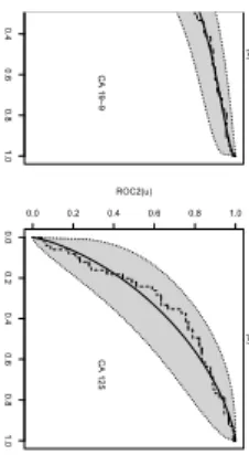
between two areas with the p-value 0.02. To visualize the sampling variability of estimated ROC curves, simultaneous ROC bands were constructed using the result in Theorem 3. Figure 2 shows the estimated ROC curves and their simulta-neous bands. These ROC curves fit very close to the empirical curves. Although our results on ROC curves and their areas show that two biomarkers are different, it is clear in Figure 3 that two ROC curves intercept. The simultaneous bands can help us determine the region of FPRs where two ROC curves are different. Figure 3 shows overlapped confidence bands. It is obvious that the ROC curve for CA 19-9 is significantly better than that for CA 125 when the false positive rate is less than around 0.17, and two ROC curves do not have much difference elsewhere.
Insert Figures 2-3 here.
7. Discussion
The interaction terms in our multivariate ROC model are completely differ-ent from the interactions of the K diagnostic tests on the measurement level. In fact, the interactions we refer to are between test types and FPRs. Multi-variate ROC models such as multiMulti-variate binormal models play an important role in ROC analysis of clustered biomarkers. This article derived asymptotic covariances of the LS, GLM and GEE estimators for multivariate ROC models with the presence of interaction terms between biomarker type and FPRs. We developed three theorems in this paper. Theorems 1-2 were developed mainly for the LS procedure. We applied some results in empirical process theory to show the asymptotic properties in Theorems 1 and 2. We then derived the asymptotic properties of correlated ROC curves with interaction terms in the model. To our knowledge, such asymptotic properties with correlated data have not been ad-dressed in empirical process theory. Theorem 3 for confidence bands can be used with all three aforementioned estimators with their respective variance estimates. The confidence band method gave an intuitive way to visualize the variability of ROC curves and the difference between ROC curves.
Due to the nature of these aforementioned ROC methods, no matter which baseline biomarker is selected, the estimated ROC curves remain the same for each of the methods. That is, all these methods respect exchangeability of base-line markers. For example, in the setting of two ROC curves, ˆθ= (ˆθ10,θˆ11,θˆ20,θˆ21)
is obtained using one of the methods when biomarker 1 is chosen as the baseline marker. The resulting estimated ROC curves are then ˜Q1(u) =g{θˆ10+ ˆθ11h(u)} for biomarker 1, and ˜Q2(u) = g[ˆθ10+ ˆθ20 +{θˆ11+ ˆθ21}h(u)] for biomarker 2. Suppose now we instead choose biomarker 2 as the baseline and obtain param-eter estimate ˆθ∗ = (ˆθ∗
10,θˆ11∗ ,θˆ∗20,θˆ21∗ ). The resulting estimated ROC curves are ˜
Q∗
1(u) =g{θˆ10∗ +ˆθ11∗ h(u)}for biomarker 2 and ˜Q∗2(u) =g[ˆθ10∗ +ˆθ20∗ +{θˆ11∗ +ˆθ21∗ }h(u)] for biomarker 1. All the three parametric methods give ˆθ10 = ˆθ10∗ + ˆθ∗20, ˆθ11 = ˆ
θ∗11+ ˆθ21∗ , ˆθ10∗ = ˆθ10+ ˆθ20 and ˆθ∗10= ˆθ10+ ˆθ20. Thus the estimated ROC curves remain unchanged.
Our new contributions also include procedures to compare AUCs and ROC curves, especially when the interaction terms between FPR’s and biomarker type are present. We drew inference for pairwise comparison between ROC curves, multiple comparisons of areas under ROC curves under binormal assumptions. Our inferential procedures in Section 4 for comparing ROC curves are very gen-eral for multivariate ROC models. Besides the three estimators we discussed, if other estimators and their covariances were available, they can also be used in these procedures.
Acknowledgment
The authors would like to thank an associate editor and two referees for their constructive comments and suggestions. This work is supported in part by NIH grant R01EB005829. This report presents the findings and conclusions of the authors. It does not necessarily represent those of VA HSR&D Service.
References
Cai, T. and Moskowitz, C. (2004). Semiparametric estimation of the binormal ROC curve. Biostatistics 5, 573586.
Cai, T. and Pepe, M.S. (2002). Semi-parametric ROC analysis to evaluate biomarkers for disease. Journal of the American Statistical Association 97, 1099-1107.
DeLong, E.R., DeLong, D.M., Clarke-Pearson, D.L. (1988).Comparing the ar-eas under two or more correlated receiver operating characteristic curves: a nonparametric approach. Biometrics 44, 837-845.
Kauermann, G. and Carroll, R. J. (2001). A Note on the Efficiency of Sandwich Covariance Matrix Estimation. Journal of the American Statistical
Associa-tion 96, 1387-1396.
Metz, C.E., Wang, P., and Kronman, H. B. (1984). A new approach for testing the significance of differences between ROC curves measured from correlated data. InInformation Processing in Medical Imaging, edited by F. Deconinck, 432-445.
Metz, C.E., Herman B.A. and Shen J-H. (1998). Maximum-likelihood estimation of ROC curves from continuously-distributed data. Statistics in Medicine 17, 1033-1053.
Pepe, M.S. (2000). An interpretation for the ROC curve and inference using GLM procedures. Biometrics 56, 352-359.
Wieand, S., Gail, M.H., James, B.R. and James, K.L. (1989). A family of non-parametric statistics for comparing diagnostic markers with paired or un-paired data. Biometrika 76, 585-592.
Zhang, Z. and Pepe, M.S. (2005). A linear regression framework for receiver op-erating characteristic(ROC) curve analysis. UW Biostatistics Working Paper
Series. Working Paper 253. http://www.bepress.com/uwbiostat/paper253.
Zhang, Z. (2004). Semiparametric least squares analysis of the receiver operating characteristic curve. University of Washington Doctoral Dissertation. Zhou, X.H., McClish, D.K. and Obuchowski, N.A. (2002). Statistical Methods in
Table 1: Rejection rates (in %) with the nominal level α = 0.05 from asymptotic results LS GEE GLM m n ρ=0 0.25 0.5 0.75 ρ=0 0.25 0.5 0.75 ρ=0 0.25 0.5 0.75 50 50 3.7 6.0 3.6 6.9 13.1 11.8 14.2 11.8 15.2 16.2 14.9 10.3 50 100 4.8 4.5 3.6 7.2 6.9 7.8 7.7 6.9 9.3 8.8 10.0 8.3 50 200 4.1 6.5 4.9 5.8 5.6 5.1 5.6 4.5 5.4 5.9 4.5 5.8 100 50 5.3 5.3 5.0 6.7 16.0 14.7 12.9 13.6 15.3 14.1 11.9 11.3 100 100 5.7 5.2 6.4 6.8 8.2 8.3 9.1 8.8 11.2 9.8 10.1 9.5 100 200 4.9 5.5 4.6 5.2 4.4 4.3 4.2 5.0 4.7 5.0 5.6 5.6 200 50 5.1 6.2 4.7 4.7 16.8 14.5 16.3 13.6 18.6 15.7 14.4 13.2 200 100 4.7 5.2 4.9 5.4 9.2 9.4 8.1 10.5 11.0 11.9 9.8 11.4 200 200 4.7 4.7 5.3 5.6 5.5 4.9 4.5 4.6 5.5 4.8 5.1 6.0
The rejection rate with 1000 realizations of normal model. The 95% pre-diction interval of the rejection rate is (5.0%± 1.4%).
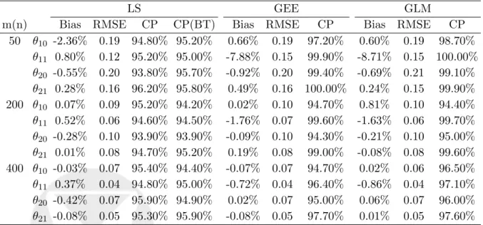
Table 2: Bias, RMSE, coverage probability (CP) of parameter estimators
LS GEE GLM
m(n) Bias RMSE CP CP(BT) Bias RMSE CP Bias RMSE CP
50 θ10 -2.36% 0.19 94.80% 95.20% 0.66% 0.19 97.20% 0.60% 0.19 98.70% θ11 0.80% 0.12 95.20% 95.00% -7.88% 0.15 99.90% -8.71% 0.15 100.00% θ20 -0.55% 0.20 93.80% 95.70% -0.92% 0.20 99.40% -0.69% 0.21 99.10% θ21 0.28% 0.16 96.20% 95.80% 0.49% 0.16 100.00% 0.24% 0.15 99.90% 200 θ10 0.07% 0.09 95.20% 94.20% 0.02% 0.10 94.70% 0.81% 0.10 94.40% θ11 0.52% 0.06 94.60% 94.50% -1.76% 0.07 99.60% -1.63% 0.06 99.70% θ20 -0.28% 0.10 93.90% 93.90% -0.09% 0.10 94.30% -0.21% 0.10 95.00% θ21 0.01% 0.08 94.70% 95.20% 0.19% 0.08 99.00% -0.08% 0.08 99.60% 400 θ10 -0.03% 0.07 95.40% 94.40% -0.07% 0.07 94.70% 0.02% 0.06 96.50% θ11 0.37% 0.04 94.80% 95.00% -0.72% 0.04 96.40% -0.86% 0.04 97.10% θ20 -0.42% 0.07 95.90% 94.90% 0.02% 0.07 95.00% 0.06% 0.07 96.00% θ21 -0.08% 0.05 95.30% 95.90% -0.08% 0.05 97.70% 0.01% 0.05 97.60% CP is the coverage percentage for 95% confidence intervals using asymptotical
standard errors with a normal quantile. CP(BT) is the coverage percentage for 95% confidence intervals using bootstrap. Results are based on 1000 realizations of bivariate normal model.
0.0 0.2 0.4 0.6 0.8 1.0 0.0 0.2 0.4 0.6 0.8 1.0 CA 125 ROC(u) u CA 19−9
Figure 1: Empirical ROC curves for CA 19-9 and CA 125: solid line, CA 19-9; dashed line, CA 125.
0.0 0.2 0.4 0.6 0.8 1.0 CA 19−9 (a) 0.0 0.2 0.4 0.6 0.8 1.0 0.0 0.2 0.4 0.6 0.8 1.0 ROC2(u) CA 125 (b)
Figure 2: Estimated ROC curves and their 95% confidence bands for CA 19-9 and CA 125: dashed lines, empirical ROC; solid lines, estimated ROC; shaded regions, 95% confidence band; dotted lines, confidence band bound-ries. 0.0 0.2 0.4 0.6 0.8 1.0 u CA 19−9 CA 125
Figure 3: Overlapped 95% confidence bands for CA 19-9 and CA 125: solid lines, estimated ROC; shaded regions, 95% confidence band; dotted lines, confidence band boundries.