logic controller for a micro robot. PhD thesis, University
of Nottingham.
Access from the University of Nottingham repository:
http://eprints.nottingham.ac.uk/12544/1/DualSurfaceType-2FLC.pdf Copyright and reuse:
The Nottingham ePrints service makes this work by researchers of the University of Nottingham available open access under the following conditions.
· Copyright and all moral rights to the version of the paper presented here belong to
the individual author(s) and/or other copyright owners.
· To the extent reasonable and practicable the material made available in Nottingham
ePrints has been checked for eligibility before being made available.
· Copies of full items can be used for personal research or study, educational, or
not-for-profit purposes without prior permission or charge provided that the authors, title and full bibliographic details are credited, a hyperlink and/or URL is given for the original metadata page and the content is not changed in any way.
· Quotations or similar reproductions must be sufficiently acknowledged.
Please see our full end user licence at:
http://eprints.nottingham.ac.uk/end_user_agreement.pdf A note on versions:
The version presented here may differ from the published version or from the version of record. If you wish to cite this item you are advised to consult the publisher’s version. Please see the repository url above for details on accessing the published version and note that access may require a subscription.
A Novel Dual Surface Type-2 Fuzzy Logic
Controller for a Micro Robot
By
Philip Birkin, BA, BSc
Thesis submitted to The University of Nottingham
for the Degree of Doctor of Philosophy
Intelligent Modelling & Analysis Research Group
School of Computer Science
The University of Nottingham
Nottingham, United Kingdom
a Micro Robot
Philip Birkin
Submitted for the Degree of Doctor of Philosophy
July 2010
Abstract
Over the last few years there has been an increasing interest in the area of type-2 fuzzy logic sets and systems in academic and industrial circles. Within robotic research the ma-jority of type-2 fuzzy logic investigations has been centred on large autonomous mobile robots, where resource availability (memory and computing power) is not an issue. These large robots usually have a variation of a Unix operating system on board. This allows the implementation of complex fuzzy logic systems to control the motors. Specifically the implementation of interval and geometric type-2 fuzzy logic controllers is of interest as they are shown to outperform type-1 fuzzy logic controllers in uncertain environments. However when it comes to using micro robots it is not practical to use type-1 and type-2 fuzzy logic controllers, due to the lack of memory and the processor time needed to cal-culate a control output value. The choice of motor controller is usually either fixed pre-set values, a variable scaled value or a PID controller to generate wheel velocities.
In this research novel ways of implementing type-1 and interval type-2 fuzzy logic controllers on micro robots with limited resources are investigated. The solution that we are proposing is the use of pre-calculated 3D surfaces generated by an off-line Fuzzy Logic System covering the expected ranges of the input and output variables. The surfaces are then loaded into the memory of the micro robots and can be accessed by the motor controller. The aim of the research is to test if there is an advantage of using type-2 fuzzy logic controllers implemented as surfaces over type-1 and PID controllers on a micro robot with limited resources.
iii
logic controllers. Each control surface was then accessed using bilinear interpolation to provide the crisp output value that was used to control the motor. Previously when this method has been used a single surface was employed to hold the information. This thesis presents the novel approach of the dual surface type-2 fuzzy logic controller on micro robots. The lower and upper values that are averaged for the classic interval type-2 controller are generated as surfaces and installed on the micro robots. The advantage is that nuances and features of both the lower and upper surfaces are available to be exploited, rather than being lost due to the averaging process.
Having conducted the experiments it is concluded that the best approach to controlling micro robots is to use fuzzy logic controllers over the classical PID controllers where ever possible. When fuzzy controllers are used then type-2 fuzzy controllers (dual or single surface) should be used over type-1 fuzzy controllers when applied as surfaces on micro robots. When a type-2 fuzzy controller is used then the novel dual surface type-2 fuzzy logic controller should be used over the classic average surface. The novel dual surface controller offers a dynamic, weighted, adaptive and superior response over all the other fuzzy controllers examined.
The work in this thesis is based on research carried out at theIntelligent Modelling and Analysis (and, originally, the Automated Scheduling, Optimisation and Planning) Re-search Group, The School of Computer Science, The University of Nottingham, England. No part of this thesis has been submitted elsewhere for any other degree or qualification and it all my own work unless referenced to the contrary in the text.
Copyright © 2010 by Philip Birkin.
“The copyright of this thesis rests with the author. No quotations from it should be pub-lished without the author’s prior written consent and information derived from it should be acknowledged”.
Acknowledgements
Firstly, I would like to express my gratitude to my supervisor, Dr. Jon Garibaldi, for providing support, guidance and opportunities throughout my PhD and who has made it possible to complete this work. I am extremely grateful for his valuable comments and the help he has afforded throughout my research.
In particular, I would like to thank Dr. Peer-Olaf Siebers for the help, encouragement and advice that he provided during my research. I would also especially like to thank Dr. Amanda Whitbrook for her help and advice, together with Dr. Joe Baxter, Dr. William O. Wilson, Dr. Robert Foster Oates (boB) and Dr. Julie Greensmith.
I would also like to thank the staff and all students of the IMA/ASAP Groups at the University of Nottingham. Thank you for creating a warm and friendly environment for academic research.
Finally, I would like to express my sincerest thanks and deepest gratitude to my wife, Margaret Mary Kenney, and to my parents Stanley and Teresa Birkin and families, who have provided their deep love and unfailing encouragement throughout my studies. They had a lot to put up with.
Abstract ii
Declaration iv
Acknowledgements v
1 Introduction 1
1.1 Fuzzy Logic Systems . . . 1
1.1.1 Applications of Fuzzy Logic . . . 5
1.1.2 Fuzzy Logic Controller Development . . . 5
1.1.3 Other Robot Controllers . . . 5
1.1.4 Robot Football . . . 6
1.2 Motivation . . . 6
1.3 Research Aims and Objectives . . . 7
1.4 Organisation of the Thesis . . . 9
2 Literature Review 11 2.1 Theory of Fuzzy Sets and Systems . . . 11
2.1.1 Classical Set Theory . . . 12
2.1.2 Boolean Logic . . . 15 2.1.3 Boolean Tautologies . . . 16 2.1.4 Fuzzy Sets . . . 18 2.1.5 Fuzzy Operators . . . 20 2.1.6 Fuzzy Logic . . . 24 2.1.7 Defuzzification . . . 27 vi
Contents vii
2.1.8 Fuzzy Inference and Reasoning . . . 28
2.1.9 Fuzzy Inferencing Systems (FIS) . . . 29
2.2 Type-2 Fuzzy Logic Systems . . . 30
2.2.1 General Type-2 Fuzzy Sets . . . 33
2.2.2 Operations on General Type-2 Fuzzy Sets . . . 36
2.2.3 General Type-2 Fuzzy Logic Systems . . . 37
2.2.4 Consequent Sets Combination . . . 40
2.2.5 The Generalised Centroid Calculation . . . 44
2.2.6 General Type-2 Centroid Type-Reduction . . . 45
2.3 Interval Type-2 Fuzzy Logic . . . 46
2.3.1 The Footprint of Uncertainty . . . 47
2.3.2 Interval Type-2 Lower and Upper Membership Functions . . . 48
2.3.3 Meet and Join of Interval Type-2 Fuzzy Sets . . . 50
2.3.4 The Interval Type-2 Inference Process . . . 51
2.3.5 Interval Type-2 Type Reduction and Defuzzification . . . 52
2.4 Architectures of Robotic Systems . . . 53
2.4.1 Subsumption Architecture . . . 53
2.4.2 Motor Schema Based Systems . . . 57
2.4.3 Other Architectures . . . 61
2.5 Robotic Strategy Methods . . . 62
2.5.1 Potential Fields (PF) . . . 63 2.5.2 Neural Networks (NN) . . . 63 2.5.3 Fuzzy Systems (FS) . . . 64 2.5.4 Rule-Based Systems (RB) . . . 64 2.5.5 Reactive Systems (RS) . . . 64 2.5.6 Other Methods . . . 65 2.6 PID Control . . . 68 2.7 Robot Football . . . 69
2.8 Potential Areas of Research Interest . . . 70
2.9 Recent Work on Type-2 Fuzzy Sets and Systems . . . 73
2.10 Summary . . . 78
3 Experimental Setup 79 3.1 Laboratory Environment . . . 79
3.2 Miabot Robots . . . 80
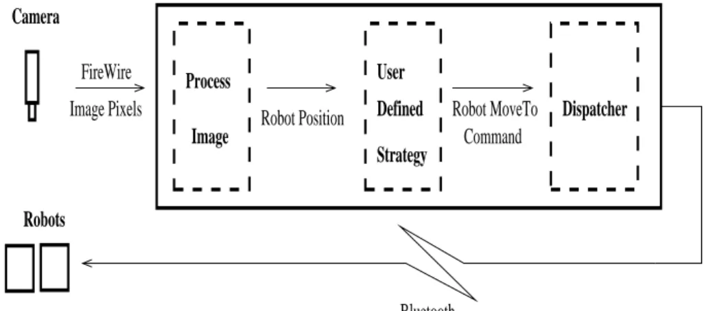
3.3 Robot Soccer Engine . . . 81
3.4 Fuzzy Inference System . . . 86
3.4.1 DC Motor Model Setup . . . 88
3.5 Independent PID Controller . . . 89
3.6 The Strategies . . . 89
3.6.1 Case Based Strategy . . . 90
3.7 Problems Discovered During Experimentation . . . 90
3.7.1 Lighting . . . 90
3.7.2 Camera Frame Speeds . . . 90
3.7.3 Physical Damage . . . 91
3.7.4 Robot Control Parameters . . . 91
3.7.5 Impact . . . 91
3.8 Robot Framework and PID Controller . . . 92
3.8.1 Initialization . . . 92 3.8.2 Command Support . . . 93 3.8.3 Communication . . . 93 3.8.4 Motor Control . . . 95 3.8.5 Control Algorithm . . . 95 3.9 Summary . . . 97
4 Development of Baseline PID Controller 98 4.1 Introduction . . . 98
4.2 No Load Encoder Clix to Power Curve Experiment . . . 98
4.2.1 Setup . . . 99
4.2.2 Discussion . . . 100
4.2.3 Conclusion . . . 102
Contents ix
4.3.1 Setup . . . 103
4.3.2 Discussion . . . 103
4.3.3 Conclusion . . . 106
4.4 Robot PID Tuning Experiment . . . 107
4.4.1 Setup . . . 108
4.4.2 Discussion . . . 108
4.4.3 Conclusion . . . 111
4.5 Summary . . . 111
5 Evaluation of Membership Functions for Type-1 and Type-2 Fuzzy Logic Controllers 113 5.1 Introduction . . . 113
5.2 Evaluation of Alternatives for Fuzzy Logic Controllers . . . 114
5.2.1 Running the Simulator for Seven Term Controllers . . . 117
5.3 Selection of Type-1 and Type-2 controllers . . . 119
5.3.1 Five and Three Term Type-2 Membership Functions . . . 121
5.4 Running the Simulator for Seven, Five and Three Term Controllers . . . . 122
5.4.1 FLC Step Change RMSE Results . . . 122
5.4.2 FLC Inertia Change RMSE Results . . . 124
5.4.3 FLC Statistical Analysis . . . 124
5.4.4 PID Controller Step and Inertia Results . . . 125
5.4.5 Comparison of Type-2 Controllers with Type-1 and PID . . . 126
5.5 Discussion . . . 128
5.6 Summary . . . 129
6 The Investigation of Single/Dual Surfaces for Type-2 Fuzzy Logic Controllers131 6.1 Setup . . . 132
6.1.1 Seven Term and Three Term Fuzzy Logic Rules . . . 132
6.1.2 Seven Term Membership Function Parameters and Shapes . . . . 133
6.1.3 Three Term Membership Function Parameters and Shapes . . . . 133
6.2 Controller Surfaces . . . 134
6.2.2 Three Term Membership Function Surfaces . . . 135
6.3 Simulator Experiments . . . 135
6.3.1 Simulation Inputs . . . 135
6.4 Type-1 and Type-2 Seven and Three Term FLC Simulation Experiments . 136 6.4.1 Experiment Comparing Type-2 and Type-1 FLCs without Noise . 136 6.4.2 Simulation Results . . . 136
6.4.3 Experiment Comparing Type-2 and Type-1 FLCs with Noise . . . 138
6.4.4 Simulation Results . . . 139
6.4.5 Experiment Comparing Type-2 FLCs with Varying Membership Thresholds and Noise Levels . . . 142
6.4.6 Simulation Results . . . 143
6.5 Discussion . . . 145
6.6 Dual Surface Seven Term and Three Term FLC Simulation Experiments . 145 6.6.1 Introducing the Dual Surface Type-2 Fuzzy Logic Controller . . . 145
6.6.2 The Dual Surface Average Threshold Mechanism . . . 146
6.6.3 The Dual Surface Weighted Average Mechanism . . . 146
6.6.4 Experimental Setup . . . 147
6.6.5 Seven Term Dual Surface Fuzzy Logic Controller . . . 147
6.6.6 Simulation Results for Seven Term Dual Surface FLC . . . 148
6.6.7 Three Term Trapezoidal Dual Surface Fuzzy Logic Controller . . 150
6.6.8 Three Term Trapezoidal Triangular Dual Surface FLC with Min-imum Implication . . . 151
6.6.9 Three Term Trapezoidal Triangular Dual Surface FLC with Prod-uct Implication . . . 152
6.7 Discussion . . . 155
6.8 Summary . . . 157
7 Evaluation of Single and Dual Surfaces in the Real World 159 7.1 Introduction . . . 159
7.2 How surfaces are generated and how they hold information . . . 161
7.3 Bilinear Access of Surface Arrays in the Micro Robot . . . 164
Contents xi
7.4.1 Background . . . 167
7.4.2 Method . . . 167
7.4.3 Results of the LED Detection Test . . . 168
7.4.4 Conclusion . . . 168
7.5 Method for Comparing the Controllers . . . 168
7.5.1 Results for Comparing the Controllers . . . 171
7.6 Introduction to Dual Surface Type-2 Controller . . . 173
7.6.1 Method for The Threshold Dual Surface Controller . . . 173
7.6.2 Results for the Threshold Dual Surface Controller . . . 174
7.6.3 Method for the Minimum and Maximum Dual Surface Controllers 175 7.6.4 Results for the Minimum and Maximum Dual Surface Controllers 176 7.7 Comparison of Three Controllers . . . 176
7.8 Method . . . 176
7.8.1 Observations . . . 177
7.9 Results . . . 177
7.10 Statistical Analysis of the Real World Robot Controllers . . . 178
7.10.1 First Group Analysis - PID Controllers . . . 178
7.10.2 Second Group Analysis - All Controllers . . . 181
7.10.3 Second Group Analysis - All robots and controllers . . . 184
7.10.4 Third Group Analysis - Type-2 Fuzzy Logic Controllers . . . 185
7.11 Discussion . . . 190 7.12 Summary . . . 190 8 Conclusions 192 8.1 Contributions . . . 192 8.2 Limitations . . . 195 8.3 Future Work . . . 196 8.3.1 Expectation . . . 197 8.4 Dissemination . . . 197
8.4.1 Refereed Conference Papers . . . 197
Appendix 213
A Chapter 3 Tables 213
A.1 Maibot Hardware Specification . . . 213
B Chapter 4 Tables 215
C Chapter 5 Membership Function Shapes, Surfaces and Tables 226 D Chapter 6 Membership Functions, Surfaces and Tables 257 E Chapter 7 Tables and Results 307
List of Figures
1.1 a) the Crisp Set Tall. b)The Type-1 Fuzzy Set Tall. . . 3
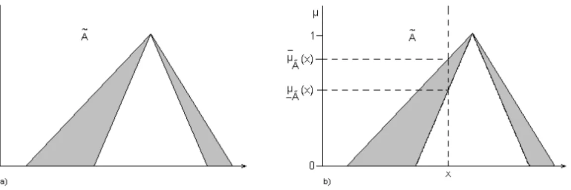
2.1 a) The Type-2 Interval Fuzzy Set ˜A. b) The Membership Grade of a Point x in ˜A. . . 47
2.2 Footprint of Uncertainty for Gaussian primary membership function with uncertain standard deviation. . . 48
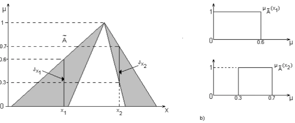
2.3 a) The FOU for a Type-2 Fuzzy Set ˜A. b) Secondary Membership Func-tions for the pointsx1andx2in ˜A. . . 50
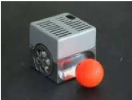
3.1 Maibot Pro BT’ Robot . . . 80
3.2 Robot Soccer Engine Overview . . . 82
3.3 Robot Player Caps . . . 84
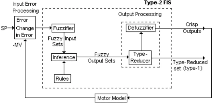
3.4 Type-2 FLC Schema . . . 87
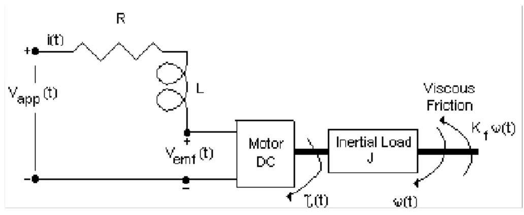
3.5 DC-Motor Model . . . 89
4.1 Histograms of No Load PWM Motor Average Clixs . . . 101
4.2 Comparisons of Load and No Load Motor Responses . . . 104
4.3 Histograms of Loaded PWM Motor Average Clixs . . . 105
4.4 Pwm Overview for PID Parameters . . . 110
7.1 Lower and Upper Dual Surfaces . . . 162
7.2 Average Type-2 and Type-1 Surfaces . . . 163
7.3 Difference Between Upper Surface and Lower Surface . . . 163
7.4 Difference between Average Type-2 Surface and Type-1 Surface . . . 164
7.5 Bilinear Interpolation Sample Space . . . 165
7.6 Box Plots of PID Controller Response without Ramp . . . 179 xiii
7.7 Box Plots of PID Controller Response with Ramp . . . 180
7.8 Robot 1 Controller Response without Ramp . . . 182
7.9 Robot 1 Controller Response with Ramp . . . 183
7.10 All Controllers Response at Speeds 10,20,40 and 80 without Ramp . . . . 186
7.11 Dual Surface and Average Response for Robot 1 only with Ramp . . . 187
7.12 Dual Surface and Average Response for 3 Robots with Ramp . . . 188
C.1 Type-1 Seven Term Gaussian Membership Shapes and Surface . . . 227
C.2 Type-1 Seven Term Trapezoidal Membership Shapes and Surface . . . 228
C.3 Type-1 Seven Term Triangular Membership Shapes and Surface . . . 229
C.4 Type-1 Seven Term Trapezoidal Triangular Membership Shapes and Surface230 C.5 Type-2 Seven Term Gaussian Membership Shapes and Surface . . . 233
C.6 Type-2 Seven Term Trapezoidal Membership Shapes and Surface . . . 234
C.7 Type-2 Seven Term Triangular Membership Shapes and Surface . . . 235
C.8 Type-2 Seven Term Trapezoidal Triangular Membership Shapes and Surface236 C.9 Type-1 Five Term Trapezoidal Triangular Membership Shapes and Surface 238 C.10 Type-1 Three Term Trapezoidal Triangular Membership Shapes and Surface242 C.11 Type-1 Three Term Trapezoidal Membership Shapes and Surface . . . 243
C.12 Type-2 Five Term Trapezoidal Triangular Membership Shapes and Surface 244 C.13 Type-2 Three Term Trapezoidal Triangular Membership Shapes and Surface246 C.14 Type-2 Three Term Trapezoidal Membership Shapes and Surface . . . 248
C.15 Type-1 and Type-2 Overview Responses with PID . . . 249
C.16 Type-1 Response Overview . . . 250
C.17 Type-2 Response Overview . . . 250
C.18 Fuzzy Logic Controllers Step Response Overview . . . 251
C.19 Fuzzy Logic Controllers Inertia Response Overview . . . 251
C.20 Type-1 Step Response Overview . . . 252
C.21 Type-1 Inertia Response Overview . . . 252
C.22 Type-2 Step Response Overview . . . 253
C.23 Type-2 Inertia Response Overview . . . 254
C.24 PID and Type-2 with PID Overview Responses with Noise . . . 254
List of Figures xv
C.26 Type-1 and Type-2 Overview Inertia Responses with PID and Noise . . . 255
D.1 Type-2 Seven Term Trapezoidal with Threshold - 1 . . . 259
D.2 Type-2 Seven Term Trapezoidal with Threshold - 0.9 . . . 260
D.3 Type-2 Seven Term Trapezoidal with Threshold - 0.8 . . . 261
D.4 Type-2 Three Term Trapezoidal with Threshold - 1 . . . 263
D.5 Type-2 Three Term Trapezoidal with Threshold - 0.9 . . . 264
D.6 Type-2 Three Term Trapezoidal with Threshold - 0.8 . . . 265
D.7 Type-2 Three Term Trapezoidal Triangular 300 with Threshold - 1 . . . . 267
D.8 Type-2 Three Term Trapezoidal Triangular 300 with Threshold - 0.9 . . . 268
D.9 Type-2 Three Term Trapezoidal Triangular 300 with Threshold - 0.8 . . . 269
D.10 Type-2 Three Term Trapezoidal Triangular 305 with Threshold - 1 . . . . 271
D.11 Type-2 Three Term Trapezoidal Triangular 305 with Threshold - 0.9 . . . 272
D.12 Type-2 Three Term Trapezoidal Triangular 305 with Threshold - 0.8 . . . 273
D.13 Type-2 Seven Term Trapezoidal Min Surfaces . . . 274
D.14 Type-2 Seven Term Trapezoidal Product Surfaces . . . 275
D.15 Type-2 Three Term Trapezoidal Min Surfaces . . . 276
D.16 Type-2 Three Term Trapezoidal Product Surfaces . . . 277
D.17 Type-2 Three Term Trapezoidal Triangular 300 Min Surfaces . . . 278
D.18 Type-2 Three Term Trapezoidal Triangular 300 Product Surfaces . . . 279
D.19 Type-2 Three Term Trapezoidal Triangular 305 Min Surfaces . . . 280
D.20 Type-2 Three Term Trapezoidal Triangular 305 Product Surfaces . . . 281
2.1 Summary of classical set theory operator properties . . . 15
2.2 An example Boolean logic truth table. . . 16
2.3 Number of Hits in Google for Robot Soccer Strategies . . . 67
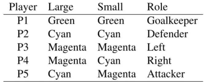
3.1 Player Identification and Role . . . 83
3.2 Colour Definition at Intensity of 120 . . . 83
4.1 No Load Mean Clix for Selected Motor PWM Demands . . . 99
4.2 Loaded Mean Clix for Selected Motor PWM Demands . . . 100
5.1 Seven Term Fuzzy Logic Controller . . . 114
5.2 Results for Seven Term Controllers . . . 118
5.3 Five Term Fuzzy Logic Controller . . . 119
5.4 Three Term Fuzzy Logic Controller . . . 120
5.5 Step RMSE for 7, 5 and 3 Term Controllers . . . 123
5.6 Step Change RMSE Means and SDs . . . 123
5.7 Inertia RMSE for 7, 5 and 3 Term Controllers . . . 125
5.8 Inertia RMSE 7, 5 and 3 Terms Means and SDs . . . 125
5.9 Mean and SD of All FLCs . . . 126
6.1 Seven Term Fuzzy Logic Controller . . . 132
6.2 Three Term Fuzzy Logic Controller . . . 132
6.3 MF Run Numbers for Type-1 and Type-2 FLCs . . . 136
6.4 Type-1 FLCs against Type-2 . . . 137
6.5 Type1 against Type-2 within Inertia . . . 138
6.6 RMSE for Type-1 and Type-2 FLCs with Noise . . . 140 xvi
List of Tables xvii
6.7 RMSE for Type-1 and Type-2 FLCs with Noise . . . 141
6.8 T2Trap7 RMSE for Dual Surface Average Thresholds within Membership Thresholds . . . 149
6.9 T2Trap3 RMSE for Dual Surface Average Thresholds within Membership Thresholds . . . 150
6.10 Minimum T2Tri300 for Dual Surface Average Thresholds within Mem-bership Thresholds . . . 152
6.11 Type1 and Average Interval Type2 RMSE Comparison . . . 152
6.12 RMSE for the Dual Surface Controller without Noise . . . 153
6.13 RMSEs for the Dual Surface Controller with Noise . . . 154
7.1 Simulation Results for Dual Surface Selection . . . 161
7.2 Hypothesis Tests for PID Controllers . . . 178
7.3 Hypothesis Tests for PID,AveT2,T1 and DST2 Controllers on Robot 1 . . 184
7.4 Hypothesis Tests for PID,AveT2,T1 and DST2 Controllers across Robots 185 7.5 Hypothesis Tests for Dual Surface and Average Response for Robot 1 only with Ramp . . . 189
7.6 Hypothesis Tests Dual Surface and Average Response for 3 Robots with Ramp . . . 189
A.1 Robot Specification . . . 214
B.1 No Load Mean and SD Clix for Left and Right Motor PWM Demands . . 216
B.2 Loaded Mean and SD Clix for Left and Right Motor PWM Demands . . . 216
B.3 Robot Response to Proportional Action . . . 217
B.4 Robot Response to Proportional and Integral Action . . . 218
B.5 Robot Response to Proportional(40),Integral and Differential Action . . . 219
B.6 Robot Response to Proportional(50),Integral and Differential Action . . . 220
B.7 Robot Response to Proportional(60),Integral and Differential Action . . . 221
B.8 Robot Response to Proportional(70),Integral and Differential Action . . . 222
B.9 Robot Response to Proportional(80),Integral and Differential Action . . . 223
B.10 Robot Response to Proportional(100),Integral and Differential Action . . 224
C.1 Seven Term Type-1 and Type-2 Gauss Parameters . . . 231
C.2 Type-1 Seven Term Trapezoidal MF Parameters . . . 231
C.3 Type-1 Seven Term Triangular MF Parameters . . . 232
C.4 Type-1 Seven Term Trapezoidal Triangular1 MF Parameters . . . 232
C.5 Type-2 Seven Term Trapezoidal MF Parameters . . . 237
C.6 Type-2 Seven Term Triangular MF Parameters . . . 239
C.7 Type-2 Seven Term Trapezoidal Triangular1 MF Parameters . . . 240
C.8 Type-1 Five Term Trapezoidal Triangular1 MF Parameters . . . 240
C.9 Type-1 Three Term Trapezoidal Triangular1 MF Parameters . . . 241
C.10 Type-1 Three Term Trapezoidal MF Parameters . . . 241
C.11 Type-2 Five Term Trapezoidal Triangular1 MF Parameters . . . 245
C.12 Type-2 Three Term Trapezoidal Triangular1 MF Parameters . . . 247
C.13 Type-2 Three Term Trapezoidal MF Parameters . . . 249
C.14 Key to Type-1 and Type-2 FLC Response Graphs . . . 253
C.15 Step Change Response Results . . . 255
C.16 Inertia Change Response Results . . . 256
C.17 PID Response Results . . . 256
D.1 Type-2 Seven Term Trapezoidal MF Parameters . . . 258
D.2 Type-2 Three Term Trapezoidal MF Parameters . . . 262
D.3 Type-2 Three Term Trapezoidal Triangular 300 MF Parameters . . . 266
D.4 Type-2 Three Term Trapezoidal Triangular 305 MF Parameters . . . 270
D.5 Simulator Input . . . 276
D.6 MF Run Numbers for Type-1 and Type-2 FLCs with Noise . . . 282
D.7 MF Run Numbers for Type-2 Thresholds . . . 282
D.8 Varying Thresholds with Inertia and No Noise for Type-2 Membership Functions . . . 283
D.9 Noise within Threshold within MF . . . 284
D.10 MF within Threshold within Noise . . . 285
D.11 Noise within MF within Threshold . . . 286
D.12 Threshold within MF within Noise . . . 287
List of Tables xix
D.14 Type1 against Type-2 within Inertia (Full) . . . 289
D.15 Type-1 against Type-2 with Noise (Full) . . . 290
D.16 Varying Thresholds with Inertia for Type-2 Membership Functions (Full) 291 D.17 Noise within Threshold within MF (Full) . . . 292
D.18 Noise within MF within Threshold (Full) . . . 293
D.19 Threshold within MF within Noise (Full) . . . 294
D.20 MF within Threshold within Noise (Full) . . . 295
D.21 Results Tri3 Test6 Product Rule, MF thresholds . . . 296
D.22 Results Tri3 Test 6 Min rule MF Th=1, DS Th Varied . . . 296
D.23 Results Tri3 Test 6 Min rule MF Th=0.9, DS Th Varied . . . 297
D.24 Results Trap3 Test 6 Min rule MF Th=1,0.9,0.8, DS Th Varied . . . 298
D.25 Results Trap7 Test 6 Min rule MF Th=1,0.9,0.8, DS Th Varied . . . 299
D.26 Results Tri3 Test 6 Min rule MF Th=1,0.8, DS Th Varied . . . 300
D.27 Type-1 Trap Ramp and Step . . . 301
D.28 Type-1 Tri Ramp and Step . . . 301
D.29 Type-2 Trap Ramp,Step and Threshold . . . 302
D.30 Type-2 Tri Ramp,Step and Threshold . . . 303
D.31 Type-1 Seven MF Trap Ramp and Step . . . 304
D.32 Type-2 Seven MF Trap Ramp and Step . . . 305
D.33 Type-2 Seven MF Trapezoidal Threshold . . . 306
E.1 Simulation Results for Dual Surface Selection . . . 308
E.2 Lower Surface for Dual Type-2 Controller . . . 309
E.3 Upper Surface for Dual Type-2 Controller . . . 310
E.4 Average Type-2 Surface for Miabot Controller . . . 311
E.5 Type-1 Surface for Miabot Controller . . . 312
E.6 Difference Between Upper Surface and Lower Surface . . . 313
E.7 Difference between Average Type-2 Surface and Type-1 Surface . . . 314
E.8 Key to Tests for Three Controller Comparison . . . 315
E.9 Results for Three Controller Comparison Tests . . . 316
E.10 Means and SDs by Controller . . . 317
E.12 Results for Threshold = 70, No Ramp . . . 318
E.13 Results for Threshold = 70, Ramp Applied . . . 319
E.14 Mean and SD for the Dual Surface Type-2 Controller - Threshold=70 . . 320
E.15 Mean and SD for the Average Type-2 Controller . . . 320
E.16 Results for Minimum Dual Controller with Ramp . . . 320
E.17 Results for Maximum Dual Controller with Ramp . . . 321
E.18 Threshold Results - for Experiment 109 . . . 321
E.19 Robot mean speed and standard deviation for each controller type . . . . 322
Chapter 1
Introduction
This thesis reports on the research carried out and the results obtained by applying type-2 fuzzy logic systems to micro robots with limited on-board memory and CPU power. In particular it is concerned with developing a type-2 fuzzy logic controller which can successfully control a micro robot with limited on-board memory and CPU power in the real world. This research proposes a novel dual surface controller type 2 fuzzy logic controller which outperforms the standard interval type-2 fuzzy logic controller, and as such, is a significant contribution to the sphere of fuzzy logic controllers.
In this chapter the main issues that the research addresses are set out. The reasons why generally type-2 fuzzy logic systems produce better models than type-1 fuzzy logic systems is discussed. The application of fuzzy logic and fuzzy logic controller develop-ment, together with other robot controllers are identified. The motivation for this research is given together with its aims and objectives. The final part of the chapter is the organi-sation of the rest of the thesis.
1.1
Fuzzy Logic Systems
Since the publishing of the seminal work “Fuzzy Sets” by Lotfi Zadeh in 1965 [1], there has been considerable progress in the development of fuzzy logic systems over the past 45 years [2]. However the ability of type-1 fuzzy logic sets to model uncertain concepts has increasingly been questioned. Researchers are frequently proposing the use of type-2 fuzzy sets as a richer model of uncertainty.
Type-1 Fuzzy Logic Systems
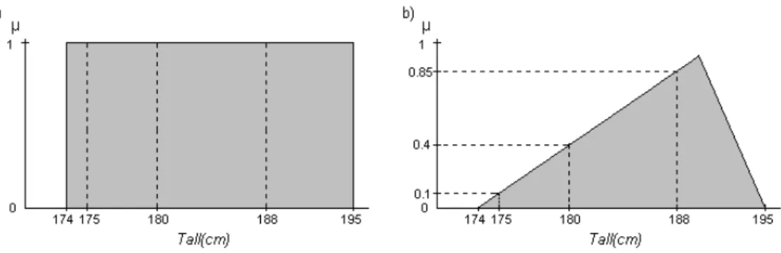
A crisp set reports assertions to be binary true or false. Either you are a member of the set or not. The crisp set Tall is depicted in Figure 1.1a) by a function, called the membership function that describes the crisp set Tall. The set Tall is defined by its membership func-tion to be a height measurement≥ 174cm and≤ 195cm. So heights of 175cm, 180cm and 188cm are all members of Tall. However the set does not report the fact that some members are taller than others, so this information cannot be modelled by a crisp set. There are many examples where degrees of category are modelled as crisp sets, such as warm, long and fast. Fuzzy sets have the property that their members can have continuous membership values [0,...,1]. The boundaries are graduated and membership of the sets can be partial. In our crisp set Tall, a height of 175cm would be classified as Tall. A casual observer might be uncertain if the person as tall, but be tempted to put them into the set Tall. Fuzzy assertions however are not binary true or false, but have a degree of truth. Due to the property that fuzzy sets have a graduated boundary, Aristotle’s Law of the excluded middle,A∪ ¬A=X, is broken. This allows all heights to be members or non-members of the fuzzy set Tall. Figure 1.1b) describes the fuzzy set Tall, by its membership function. Now there is a way to capture and model this type of data representation. In our exam-ple a person of 180cm could be a member of Tall with a membership grade of 0.4. The person of height 188cm could have a membership grade of 0.85 and the 175cm person could be a member with membership grade of 0.1. If we have another type of height called Medium then the height of 175 could have a membership grade of 0.8, 180cm a membership grade of 0.3 and 188cm a membership grade of 0. The height information that could not be modelled by a crisp set can now be modelled by a fuzzy set. This can be applied to any vague concept. This leads to an understanding of the concept of vagueness to be something that cannot be adequately modelled by a crisp set. Fuzzy logic systems are based upon knowledge that is captured in fuzzy sets and rules. Using actual facts and observations, the process of reasoning and making decisions is provided. Due to being able to model the vagueness of a concept with a fuzzy set, an improvement in the decision making process occurs.
In order to use fuzzy sets type-1 fuzzy logic systems have extended the crisp logi-cal operators ‘and’, ‘or’ and ‘implies’. This allows the processing of fuzzy production
1.1. Fuzzy Logic Systems 3
Figure 1.1: a) the Crisp Set Tall. b)The Type-1 Fuzzy Set Tall.
rules to occur. During the inference processing, when a rule is fired then it is fired to a degree. This means that the vagueness of the variables is passed on, in keeping with the original meaning. In ‘Computing with Words’ [3] Zadeh expected that fuzzy systems and computing in general would be able to use natural language to describe and execute requirements. However the reality is that fuzzy logic systems are dominated by control system applications.
One of the drawbacks of type-1 fuzzy logic, is concerned with the concept of uncer-tainty. Uncertainty is understood to be when the boundaries of a concept are vague. A type-1 fuzzy logic cannot capture uncertainty only vagueness. In our example a height of 188cm is 0.85 in Tall requires that everything about the concept Tall is known and an accurate model exists. In the Baltic states the average height is higher than the UK, so the environment where the measurement takes place introduces uncertainty. Also a group of experts might disagree as to the value of 0.85 membership grade for 188cm, and also their opinions can alter over time.
Type-2 Fuzzy Logic Systems
In order to capture uncertainty the type-1 fuzzy logic system has to be extended. In our example - 188cm is 0.85 membership grade in the set Tall, becomes hedged with the word ’about’. This gives the statement - 188cm is about 0.85 membership grade in the set Tall. This means that the membership function of the fuzzy set has to capture the vagueness of the membership grade. This is achieved by modelling the secondary membership func-tions as type-1 fuzzy sets. So in a type-2 fuzzy set the boundaries are graduated allowing
the modelling of vagueness. The boundaries themselves are also vague about the knowl-edge of the concept, that is they are uncertain. The class of type-2 fuzzy set described here is a Generalised type-2 fuzzy set and is usually referred to as a type-2 fuzzy set.
The price of having uncertainty in the type-2 Fuzzy Logic System model is increased computation complexity. The type-1 model is based on a 2-D representation which maps the domain elements of the set to values [0,..,1]. By having the secondary membership grades as type-1 fuzzy sets, the model becomes 3-D. Now the process is to map the domain elements of the boundary graduated sets to a function which than maps onto the membership grade sets. The Cartesian product of this is potentially massive and seriously impacts and increases the complexity of type-2 systems.
In order to reduce the complexity, another method is to represent type-2 fuzzy logic systems using interval type-2 fuzzy sets. All points in each of the secondary membership functions are set at unity, so each secondary membership can be represented as an interval set. An interval set ˜A contains two elements, a lower bound which is denoted ˜Aand an upper bound denoted ˜A, such that ˜A= [A˜,A˜]. All points between these bounds are implicit elements of the interval set. By using interval type-2 fuzzy sets the processing is reduced, due to the third dimension in the interval type-2 fuzzy sets being unity and thus ignored in the computation. However this causes a loss of accuracy in the final result.
Fuzzy Logic Rule Base
Whether a type-1 or a type-2 fuzzy logic system is used the fuzzy logic rule base is the same. Fuzzy rules are of the form ‘IF antecedents THEN consequents’. The antecedents are combinations of one or more input variables, connected by the fuzzy operators ‘AND’ or ‘OR’. The consequents are types of the output variable. For example using the Mam-dani rules base:
IF Room is Hot AND Weather is Warm THEN Heating is Off IF Room is Warm AND Weather is Cold THEN Heating is Medium
The values for the types are described by membership functions which are usually defined by expert opinion. Usually this is sufficient to set up a fuzzy logic system.
1.1. Fuzzy Logic Systems 5
1.1.1
Applications of Fuzzy Logic
With the boom in consumer goods and the investments made by Japanese manufactures fuzzy logic controllers can be found in such diverse equipment as washing machines and auto focus cameras, refrigerators, photocopiers and televisions. With the development of fuzzy programmable logic controllers by companies like Moeller, the industrial applica-tion of fuzzy logic is ever growing. In fact wherever decisions have to be made such as data analysis or signal processing, fuzzy logic can be used to make them. In the industrial world fuzzy logic has been used to solve many problems, these include Power Genera-tion, Turbine Engine Control, Heating, Pumping, Air Conditioning, Electric Motor and Voltage Regulation and Motion Control.
1.1.2
Fuzzy Logic Controller Development
The first practical use of fuzzy logic was by Mamdani and Assilian in 1974/5 [4]. They successfully used fuzzy logic to control a steam engine. In 1977 Siemens used a fuzzy set concept to control traffic lights [5]. The first industrial application was in Denmark. The purpose was to control a cement kiln. The project was started in 1976 and was completed in 1982 [6]. Yasunobu working for Hitachi in Japan started work in 1979 on a project to control the subway trains of Sendai [7]. The system was successfully commissioned in 1987. Following a development program, Fuji Electric offered the first commercial fuzzy logic controller in 1985.
1.1.3
Other Robot Controllers
In non-reactive architectures robot controllers provide the reasoning on what to do. Too close then move away, or nothing near then go faster. Many different controllers have been proposed over the years, including Neural Networks [8], Potential Field [9], Fuzzy Logic [10], Sensor Fusion [11], and more recently Artificial Immune Systems [12, 13] and Idiotypic Networks [14,15] carried out at the University of Nottingham. However the reason for selecting fuzzy logic systems as the controllers of choice for the research was the wealth of departmental expertise in the field of fuzzy logic systems.
1.1.4
Robot Football
There are two organisations that are concerned with robot football, The RoboCup Fed-eration1 and FIRA (Federation of International Robot-soccer Association)2. The aim of the RoboCup project is ‘By 2050, develop a team of fully autonomous humanoid robots that can win against the human world champion team in soccer’. Robot football is played in many different configurations including humanoid robots. Each league is governed by a comprehensive set of rules that ensure the physical robots are matched. However the implementation of architectures and strategies are left entirely to the team designers. As demonstrated in the Dapra challenges, competition is a massive driver of progress [16]. Robot football games are fast and dynamic, especially in the FIRA mirosot leagues. The games are unpredictable and random which mirrors the real world. Due to the robots moving so quickly and colliding there are lots of failures, which the teams have to handle.
1.2
Motivation
The theme that runs through the previous discussion is that the robots are medium sized and the motors used are large. Indeed, the engine used by Hagras [17] is a marine diesel engine capable of getting a boat across the Atlantic.
In contrast, the motivation of this research is to facilitate and enable micro robots to successfully operate in a robot football team environment. In order to play robot football, the robots have to be able to move accurately at speeds of over 1msec−1 and intercept the golf ball football. They must be able to control the ball and change direction quickly. They are subject to rapid accelerations and decelerations. The environment is very harsh and very noisy, with many high speed collisions occurring with other team members and opposition robots. This real world problem is the driving force behind this research.
A major issue of the micro robots is the limited on-board memory and CPU power and the space available to hold boards and batteries within the allowed shape and size of the robots. This was solved by the manufacturers by supplying a PID controller to control the robot motors, which required very little code and a very small amount of data storage.
1www.robocup.org 2www.fira.net
1.3. Research Aims and Objectives 7
The Robot Soccer Engine (RSE) supplied to control the robots during a football match configures all the robots with the same PID parameters. However the characteristics of each robot player in the football team are different. The goalkeeper has to be able to accurately intercept or block the ball usually from a standing start, and so requires very fast reaction times. Where as a striker has to be able to control the ball and direct it towards the opponents goal, avoiding any defenders trying to block its path. The control requirements for this demand accuracy of speed and position.
The need to have different PID controllers for each player in the robot football team led to the use of PID controllers being questioned. Would a fuzzy logic controller provide an alternative solution to the problem? Having posed this question, the next question is what type of fuzzy controller to use. The possibilities were either a type-1 or a type-2 controller. This leads to the question and challenge of how to implement a fuzzy logic controller on the micro robot given the major issue of limited on-board memory and CPU power. Indeed this issue channelled the direction of the research aims and objectives and the solution that was consequently arrived at.
Generally throughout the research the motivation and aim is to produce a fuzzy logic controller that operates successfully in the real world. The major issue of having limited on-board memory and CPU power on the micro robot has a large impact by constraining the scope of the research to a solution that can be implemented under these conditions. Having shown that it is possible to develop a fuzzy logic controller for a micro robot, then it expected that the controller can be scaled up and implemented on medium and large robots successfully. The aim is ultimately to be able to implement and abstract the fuzzy logic controller onto any fuzzy logic system.
1.3
Research Aims and Objectives
The central aim for this research is to discover whether alternatives to PID control, par-ticularly fuzzy controllers of either type-1 and type-2, can make substantial, observable difference to the micro robots within a robot football environment. More specifically, could alternative controllers actually result in a better game being played by the robots. This central aim led to three specific research objectives:
1. Compare PID, type-1 and type-2 controllers on a micro robot with limited on-board memory and CPU power. Various alternative controllers were designed and then implemented in software in a form suitable to be deployed on the robot football micro robots. This meant that the computational resources of the robots were a hard constraint on the implementation process. As a result, the fuzzy controllers were implemented as static look-up tables of the control surface which was produced by the various fuzzy controllers. This led to the observation that there was no essential difference between a control surface look-up table produced from a type-1 fuzzy controller and that produced by a type-2 controller.
2. Investigate a novel dual surface type-2 controller. Following the above observation, a novel form of type-2 controller was investigated, in which the upper control sur-face and lower control sursur-face (see Chapter 6 for full explanation of these terms) were both stored within the micro robot. This allowed more of the information produced by the type-2 controller to be represented within the robot, potentially providing more sophisticated type-2 control. The results showed that in simula-tion, generally the type-2 fuzzy logic controller outperformed the equivalent type-1 controller both with and without Gaussian noise being applied to the system. Both fuzzy controllers out-performed the PID reference controller. This is consistent with the theoretical and practical observations made for simulated experiments. 3. Measure the effects of these alternative controllers on real world performance.
While much literature has examined the differences between type-1 fuzzy control and PID control, and more recently (but to a lesser extent) the additional benefits of type-2 control, often these experiments have been in terms of easily measurable parameters such as the RMSE (root-mean-squared-error) between the controller output and the required set-point. Studies of the effect of these controller differ-ences on the observable real world behaviour have been less common — does, for example, a 1% reduction in controller RMSE lead to any observable difference in behaviour? The last objective of this work was to examine the controller differ-ences in terms of whether they lead to any substantial, observable differdiffer-ences in high-level behaviour of the micro robots — essentially, are any differences in the
1.4. Organisation of the Thesis 9
controllers enough to lead to observable improvements in the ability of the robots to play football?
1.4
Organisation of the Thesis
The remainder of the thesis is organised as follows.
• Chapter 2 reviews the relevant literature covering the research domain of this thesis. The first part is concerned with common problems associated with robots. There is a detailed literature review of the architectures and systems used in multi-robot teams. Significant approaches to the solution of these problems are discussed and critically analysed. The taxonomies that are available to describe the teams are analysed. The control methodologies used in micro-robot football are explained and critically analysed. The second part of the literature review is a discussion about fuzzy logic. It origins and development as a type-1 logic and the development and advancement of type-2 fuzzy logic.
• Chapter 3 describes the environment within which the robots operate. This includes a detailed description of the robot hardware, the firmware of the robot and the soft-ware that is used to control the robots. The system specifications and configurations are detailed. The performance attributes of the robots are discussed along with prob-lems that were encountered whilst running the robots. There is a discussion about the difficulty of getting meaningful data from the robot whilst it was running. • Chapter 4 investigates the performance of the micro robots using an independent
PID controller.
• Chapter 5 describes the investigations into various alternative type-1 and type-2 fuzzy controllers, with particular emphasis on the design of membership functions. • Chapter 6 is concerned with the design of the novel dual-surface type-2 fuzzy con-troller, its associated membership functions and the simulation experiments that were carried out to evaluate its performance.
• Chapter 7 describes the real world experiments that were performed to test the re-sults obtained from the simulation. These include the real world PID experiments that were carried out to ascertain the best tuning parameter set for the robot when in PID mode. The effect of using a ramp to control the power input to the robot when in PID mode. A smoothing algorithm was trialled. A series of experiments comparing all different controllers at different power values. Also tested a voting system that picked from the upper, lower or averaged surface value, depending on the state of an error metric. A statistical breakdown of each test is given. This demonstrated that in the real world that there was no significant difference between the robot controllers.
• Chapter 8 concludes the thesis with a discussion on the contribution made and the limitations of what was done. The future work that is available and dissemination of the research.
Chapter 2
Literature Review
The previous chapter defined the goals and scope of this thesis. This chapter presents the fields of classical set theory and the theory of fuzzy sets and systems. In addition, the chapter introduces the notion of type-1 and type-2 fuzzy sets and explains their differ-ences together with the theory underpinning type-2 fuzzy sets. Architectures of robotic systems are introduced together with strategies that are available to control the robots. The PID controller is briefly reviewed as this the most common form of motor control in micro robots. Robot football, the motivation for this research is touched upon, and is then followed by an examination of potential areas of research interest. Finally recent work on type-2 fuzzy sets and systems including new methods of defuzzification are reported.
2.1
Theory of Fuzzy Sets and Systems
A fuzzy set is a generalization of a classical set, but differs in that it allows objects to take partial membership of its sets, with the real-valued degree of membership ranging from 0 to 1. Since much of the theory of fuzzy sets is rooted in classical set theory, this chapter begins with a introduction to the fundamental concepts of classical set theory and Boolean logic. It goes on to define fuzzy sets and show how they differ from classical sets. The ap-plication of Boolean logic to fuzzy sets and systems, which is known as fuzzy reasoning, is also discussed along with a description of fuzzy membership functions, fuzzy operators and defuzzification.
2.1.1
Classical Set Theory
A set is defined as a collection of unique objects termedelementsormembersof the set. In set theory, as Cantor [18] defined and Zermelo [19] and Fraenkel [20] axiomatised, an object is either a member of a particular set or not. For example, a pedigree Bengal cat is in the set of all pedigree cats, but a pedigree Pekingese dog is not. In dealing with sets it is also necessary to define auniverse of discourse, which provides the set of allowable values for objects, i.e. the relevant set of entities that are being dealt with. For example, the universe of discourse could be the set of all animals, the set of real numbers or the set of natural numbers.
In representing sets mathematically, the convention is to use capital letters for sets, and lower case letters for objects and set members. In addition, the universal set, defined as the set of all sets, is represented asU, and a set with no elements, called anull, orempty
set and is denoted as /0. A set may be defined by listing all its members (the list method), for example:
A={a1, a2, ..., an},
(wherenis the number of members of the set), or by defining the criteria that each member must meet in order to be considered a member of the set (the rule method):
A={a|ameets some condition(s)},
for example,
A={a|0≤a≤10}.
The relationship between a set Ain a universe of discourseX and an objectxis ex-pressed mathematically as:
x∈A,
ifxis a member ofAand by:
x∈/A,
if x is not a member of A. Alternatively, a zero-one membership function for A (also known as a characteristic function, discrimination function or indicator function) may be
2.1. Theory of Fuzzy Sets and Systems 13
introduced, which encapsulates the notion that an objectx∈Uis either a full member of
Aor not a member ofAat all. The membership function is denoted byµA(x)and is such that: µA(x) = 1 if and only if x∈A, 0 if and only if x∈/A.
Therefore, µA maps all elements of the universal set into the set A with values 0 and 1, which can be written in functional notation as:
µA:U→ {0,1}.
When every element in the setAis also a member of setB, thenAis said to be asubset
ofB, and this is written as:
A⊆B.
For example,{1, 2}is a subset of{1, 2, 3}, but{1, 4}is not. It thus follows that if every element inAis also inBand every element inBis also inA, i.e. A⊆BandB⊆A, then the setsAandBare equal:
A=B.
Alternatively, if at least one element in setAis not in setB, or at least one element inBis not inA, thenAandBare not equal:
A6=B.
SetAis aproper subsetofBifAis a subset ofBbutAandBare not equal, i.e.A⊆Band
A6=B. This is represented as:
A⊂B.
In this case, every element ofAis inB, butBhas additional elements not found inA. Just as arithmetic is concerned with operations on numbers, set theory is concerned with operations on sets. Some of the more common operators are summarized below:
• The unionof sets A andB, denoted byA∪B, is the set of all distinct elements in both sets. For example, the union of {1, 2, 3}and{2, 3, 4}is the set{1, 2, 3, 4}.
This is similar to the logical “OR” operator, see Section 2.1.2.
• The intersection of the setsA andB, denoted byA∩B, is the set that contains all elements of A that also belong to B (or equivalently, all elements of B that also belong to A), but no other elements. The intersection of{1, 2, 3}and {2, 3, 4}is the set{2, 3}. This is similar to the logical “AND” operator.
• The complement of setArelative to setX, denotedAc, ¯AorA′is the set of all mem-bers ofXthat are not members ofA. This terminology is most commonly employed whenX is the universal setU, as in the study of Venn diagrams. The complement
of {1, 2, 3}relative to {2, 3, 4}is{4}, while, conversely, the complement of {2, 3, 4}relative to{1, 2, 3}is{1}. This is similar to the logical “NOT” operator and can also be written as “not A” or ¬A. In classical set theory, the complement is reflexive, i. e.,¬(¬A)≡A.
• The symmetric difference between setsAand Bis the set with members that only belong to AorB. For instance, for the sets{1, 2, 3}and{2, 3, 4}, the symmetric difference is the set{1, 4}.
• The set difference between setsAandB, expressed asA−B, is the set of elements that are inA, with those that are inBsubtracted out. Therefore,A−Bis the set of elements that are inAand not inB, i. e. A−B≡A∩ ¬B. For instance, for the sets
{1, 2, 3}and{2, 3, 4}, the set difference is the set{1}.
• The Cartesian product of A and B, denoted A×B, is the set with members that represent all possible ordered pairs (a, b) where a is a member of A and b is a member ofB. For the sets {1, 2, 3}and{2, 3, 4}, the Cartesian product produces the set{(1, 2), (1, 3), (1, 4), (2, 2), (2, 3), (2, 4), (3, 2), (3, 3), (3, 4)}. The operation can be expressed mathematically as:
A×B={(a,b)|a∈A,b∈B}. (2.1)
The examples quoted above use only two sets, but it is important to note that these operators can be used on any number of sets and that they may be combined to produce
2.1. Theory of Fuzzy Sets and Systems 15
more complex operators. The mathematical properties of the union, intersection and com-plement operators are summarized in Table 2.1.
Table 2.1: Summary of classical set theory operator properties
Property Example Involution ¬¬A≡A Commutativity A∪B≡B∪A A∩B≡B∩A Associativity (A∪B)∪C≡A∪(B∪C) (A∩B)∩C≡A∩(B∩C) Idempotence A∪A≡A A∩A≡A Distributivity A∩(B∪C)≡(A∩B)∪(A∩C) A∪(B∩C)≡(A∪B)∩(A∪C) Absorption A∪(A∩B)≡A A∩(A∪B)≡A
Classical sets are often referred to as crispsets to distinguish them from fuzzy sets, see Section 2.1.4.
2.1.2
Boolean Logic
Boolean logic is named after George Boole, who first defined an algebraic system of logic in the mid 19th century. His system defines a number of logical operators, but includes only two possible truth values, true (1) and false (0). These values can be combined using the defined logical operators to produce a vocabulary of Boolean logic, which can be expressed as atruth table. An example table, which demonstrates the results of applying the logical operators AND, OR, NOT, EQUIVALENCE and IMPLICATION to variables
AandBis shown in Table 2.2 below. The operators are symbolized by standard notation, i.e.∧,∨,¬,⇔and⇒respectively.
The most simple and most commonly used operators are AND and OR. The AND operation returns true if and only if all inputs are true; i.e. the output is false if any of the
Table 2.2: An example Boolean logic truth table. A B A∧B A∨B ¬A ¬B A⇔B A⇒B 0 0 0 0 1 1 1 1 0 1 0 1 1 0 0 1 1 0 0 1 0 1 0 0 1 1 1 1 0 0 1 1
inputs are false. Alternatively, the OR operation returns true if any of the inputs are true. The NOT operator is applied to a single input and returns its opposite, i.e. false if the input is true and vice versa. The EQUIVALENCE operator returns true if two inputs are the same and false if they are different. The IMPLICATION operator is more complex and most relevant to the field of fuzzy logic, since it deals with antecedent and consequent parts of complex logical statements. When applied to two simple logical statementsA(the antecedent part of a more complex statement or thepremise) andB(the consequent part orconclusion), ifBis a logical consequence ofAthen the value ofA⇒Bis true. In fact, it is worth noting that the operator returns false only in the case where the premise is true and the conclusion is false. The logical reasoning underlying this is interpreted as:
• A true premise implies a true conclusion, therefore ifT represents true,T⇒T≡T. • A true premise cannot imply a false conclusion, thereforeT ⇒F≡F.
• Anything may be concluded from a false assumption, soF ⇒F ≡T andF ⇒T ≡
T.
Note that the IMPLICATION operator is not commutative, i.e.,A⇒B6=B⇒A.
2.1.3
Boolean Tautologies
In any particular logic system, reasoning procedure relies on tautologies, or rules that remain true in that logic system regardless of the values assigned to the variables involved. Four examples of Boolean tautologies are discussed below.
2.1. Theory of Fuzzy Sets and Systems 17
The first tautology is called modus ponens, sometimes referred to as “affirming the antecedent” or “the law of detachment”. Modus ponens states that ifP⇒Q=1 andP=1, where 1 represents true, then it can be concluded thatQ, the consequent of the conditional claim, must be true as well. As an example, supposePis the logical statement “Today is Tuesday” andQis the logical statement “I have to go to work today”. IfPimpliesQ, i.e., if the complex logical statement “If today is Tuesday then I have to go to work today” holds true andP is true, i.e. it is Tuesday, then it is also true that I have to go to work today, i.e.Qis also true. This can be expressed mathematically as:
((A⇒B)∧A)⇒B≡1. (2.2)
Equation 2.2 holds true whatever value the inputs forAandB take. In Artificial Intelli-gence, modus ponens is often called forward chaining.
The second tautology is calledmodus tollens. This can be expressed mathematically as:
((A⇒B)∧ ¬B)⇒ ¬A≡1, (2.3)
and can also be referred to as “denying the consequent”. Modus tollens states that if
P⇒Q=1 and Q=0, where 1 represents true and 0 represents false, then it can be concluded that P, the premise of the conditional claim, must be false as well. In the example above, if the complex logical statement “If today is Tuesday then I have to go to work today” holds true andQis false, i.e. I do not have to go to work today, then one can conclude that it cannot be a Tuesday, i.e.Pis false.
The third tautology is known ashypothetical syllogismand can be represented as:
((A⇒B)∧(B⇒C))⇒(A⇒C)≡1. (2.4)
This can be interpreted as “IfA impliesBand BimpliesC thenA also impliesC”. The final tautology is calledcontrapositionand is written mathematically as:
The interpretation of this tautology is that “IfAimpliesBthen¬Bimplies¬A”.
Acontradictionis the opposite of a tautology, i.e., the statement made is always false. For more information on classical logic see Klir & Folger [21].
2.1.4
Fuzzy Sets
Fuzzy sets were first introduced by Zadeh in 1965 [1] to model the imprecision and un-certainty inherent in assigning membership of elements to real-world sets, for example the set ofshortpeople or the set ofyoungpeople. The theory provided formalized tools for dealing with such imprecision or vagueness in real world applications, allowing many complex decision-making problems to be simplified.
The fuzzy set is a generalization of a crisp or classical set and is characterized by a membership function µ(x), that takes on values in the interval [0,1], as opposed to the membership functions of crisp sets that can take only the values 0 or 1, see [22]. This means that elements are permitted to take partial membership of fuzzy sets. The
membership gradeof an elementx with respect to a set Ais denoted by µA(x), withµA mapping all elements of the universal set into the set A with values in the continuous interval 0 to 1. This can be expressed in functional notation as:
µA:U→[0,1].
As with crisp sets, a fuzzy set may be defined formally using the list method. When applied to fuzzy sets, this becomes a list of the strength of membership of each element of a discrete, countable universe of discourse to the set in question, which is represented mathematically as: A= n
∑
i=1 µi/xi, (2.6) or A={µ1/x1+· · ·+µn/xn}, (2.7)2.1. Theory of Fuzzy Sets and Systems 19
of membership of elementxi andA is the set of interest. Note that the summation and addition symbols in Equation 2.6 and Equation 2.7 do not represent algebraic summation; they indicate the collection or aggregation of each element. The description of a fuzzy set on a continuous universe is written as:
A=
Z
U
µA(x)/x, (2.8)
whereU is the universe of discourse and the integral symbol represents a continuous, function-theoretic aggregation operator for continuous variables, not algebraic integra-tion [23].
An example membership function, used to assign membership values to the fuzzy set
A, which represents temperatures close to 30 °C, could be:
µA(x) = 1
1+(x−3030)2. (2.9)
Equation 2.9 maps every real number in a continuous universe of discourse into the set of temperatures close to 30 °C, for example 15°C would be assigned a membership value of 0.12, 20 °C would be assigned a membership value of 0.23 and 30 °C would have a membership value of 1.0.
Alternatively, if one is dealing with a discrete universe of discourse, for example ele-ment values between 15 and 45 in steps of five, one may express the fuzzy setAas:
A= 0.12 15 + 0.23 20 + 0.55 25 + 1.0 30 + 0.55 35 + 0.23 40 + 0.12 45 , (2.10)
for example. Equation 2.10 uses the discrete values obtained from the continuous function of Equation 2.9.
In general, the membership function can assume any shape, but those most commonly used are triangular, Gaussian, Sigmoid, and S-shaped functions.
2.1.5
Fuzzy Operators
Since fuzzy set theory is a generalization of classical set theory, its axiomatic foundation has some important differences [24]. In particular, it violates two fundamental laws of Boolean algebra; the law of excluded middle A∪ ¬A=U, where U is the universe of discourse, and thelaw of contradiction A∩ ¬A= /0. This is because it is possible for an element to have degrees of belonging both to a fuzzy set and its complement. This means that logically equivalent formula from classical set theory are not necessarily equivalent in fuzzy logic.
As discussed in Section 2.1.1, the main operators on any set, whether crisp or fuzzy are intersection, union and complement. In classical set theory these operations are uniquely defined, see [25], but in fuzzy set theory there are many different ways to define them as the operations are based on membership values, which are no longer restricted to{0,1}. However, it is important to note that any definition of these operations on fuzzy sets must include the limiting case of crisp sets. Example definitions for the above three operators are those given by Zadeh [1]:
• IntersectionA∩B: µA∩B(x) =min[µA(x),µB(x)],
• UnionA∪B:µA∪B(x) =max[µA(x),µB(x)],
• ComplementA′: µA′(x) =1−µA(x).
Other widely-used definitions include the algebraic product for intersection, see Sec-tion 2.1.5 and the algebraic sum for union, see SecSec-tion 2.1.5, but there are an infinite number of other choices. Also, it is worth noting that the selection of an intersection op-erator may influence the choice of union opop-erator due to theprinciple of dualitybetween them [24]. A fuzzy intersection operatort(x,y)and a fuzzy union operators(x,y)form a dual pair if they satisfy the following condition:
2.1. Theory of Fuzzy Sets and Systems 21
The above duality condition ensures that:
¬(A∩B)≡ ¬A∪ ¬B, (2.12)
(which is always true in classical set theory), still holds in fuzzy set theory. The appli-cation of the intersection, union, complement and impliappli-cation operators to fuzzy sets is discussed in more detail in Sections 2.1.5, 2.1.5, 2.1.5 and 2.1.5 respectively.
Fuzzy Intersection
The set of candidate fuzzy intersection operators is termedtriangular normsor t-norms
and is defined by a set of axioms. These are set out below:
A t-norm operatort(x,y)must satisfy the following conditions for anyw,x,y,z∈[0,1]:
1. t(0,0) =0,t(x,1) =t(1,x) =x(boundary condition),
2. t(x,y)≤t(z,w)ifx≤zandy≤w(monotonicity condition),
3. t(x,y) =t(y,x)(commutativity condition),
4. t(x,t(y,z)) =t(t(x,y),z)(associativity condition).
The boundary condition imposes a generalization to crisp sets and the monotonicity con-dition implies that a decrease in the membership values of sets X or Y cannot produce an increase in the membership value ofX∩Y. The commutativity condition ensures that
X∩Y ≡Y∩X, and the associativity condition permits the intersection of any number of sets in any order of pairwise groupings.
It is often useful to limit the cluster of fuzzy intersections by taking into account additional conditions as follows:
• t is a continuous function (continuity condition), • t(x,x)≤x(subidempotency condition).
Continuity avoids the situation where a small change in the degree of membership to setX
condition deals with degrees of membership of X or Y having the same value x. This axiom expresses that the degree of membership toX∩Y should not exceed the value ofx.
The most common t-norms (besides minimum) are listed below: • Algebraic product: t(x,y) =xy,
• Limited difference: [26]t(x,y) =max(0,x+y−1),
• Drastic intersection: t(x,y) = x ify=1 ; y ifx=1 ; 0 otherwise. Fuzzy Union
The set of candidate fuzzy union operators is termedtriangular conorms, t-conormsor
s-normsand is defined by the following set of axioms:
An s-norm operators(x,y)must satisfy the following conditions for anyw,x,y,z∈[0,1]: 1. s(1,1) =1,s(x,0) =s(0,x) =x(boundary condition),
2. s(x,y)≤s(z,w)ifx≤zandy≤w(monotonicity condition),
3. s(x,y) =s(y,x)(commutativity condition),
4. s(x,s(y,z)) =s(s(x,y),z)(associativity condition).
As with fuzzy intersection, it is often useful to limit the choice of fuzzy union opera-tors by imposing additional conditions as follows:
• sis a continuous function (continuity condition), • s(x,x)≤x(subidempotency condition).
The most common s-norms (besides maximum) are listed below: • Algebraic sum: s(x,y) =x+y−(xy),
• Boundary sum: s(x,y) =min(1,x+y), see [26],
• Drastic union: s(x,y) = x ify=0, y ifx=0, 1 otherwise.
2.1. Theory of Fuzzy Sets and Systems 23 Fuzzy Complement
Zadeh [1] defined membership of a fuzzy complement set as one minus the degree of membership of the original set, but there are an infinite number of other definitions for fuzzy complement operatorsc(x). Each, however, is characterized by the following ax-ioms:
1. c(0) =1,c(1) =0,
2. Ifx<ythenc(x)≥c(y);x,y∈[0,1].
The first axiom defines the boundary conditions and the second defines the fuzzy com-plement as monotonic increasing, which mimics the crisp comcom-plement. This is intuitive since, as the degree of membership of an element in set X increases, its membership in the complement set should decrease. Two further conditions are also very useful when assigning fuzzy complement operators. These are:
• cis a continuous function (continuity condition), • c(c(x)) =xfor allx∈[0,1](involution condition).
The involution constraint is imposed when the complement of a fuzzy set must be re-versible.
Fuzzy Implication
Classical set theory has only one definition of the implication operator, but an infinite number of implication operators are possible with fuzzy sets and systems. Zadeh [27] defined fuzzy implication as:
A⇒B=A×B, (2.13)
where×indicates the Cartesian product of the two fuzzy setsAandB. IfAis a subset of the universe of discourseU andBis a subset of the universe of discourseV, this can be expressed as:
A×B=
Z
U×V
where:
U×V ={(u,v)|u∈U,v∈V}, (2.15)
from Equation 2.1.
Equations 2.13 and 2.14 show that, under this particular definition of fuzzy implica-tion, the result ofA⇒Bis a fuzzy set of ordered pairs (u,v),u∈U,v∈V, and that the membership values of(u,v)are given byt(µA(u),µB(v)), where t represents some t-norm operator. As an example, suppose that:
U =4+5, (2.16)
V =5+6+7, (2.17)
A=0.5/4+0.7/5, (2.18)
B=0.4/5+0.8/6+0.3/7, (2.19)
and that the t-norm is the minimum. Then
A×B=0.4/(4,5) +0.5/(4,6) +0.3/(4,7) +0.4/(5,5) +0.7/(5,6) +0.3/(5,7).
(2.20)
There are many other commonly-used implication operators, e.g. the S-implication, QL-implication, and R-implication operators. A thorough review of fuzzy implications is presented in Dubois & Prade [28], and the use of the implication operator within fuzzy logic is discussed further in Section 2.1.6.
2.1.6
Fuzzy Logic
In fuzzy set theory, elements have degrees of membership to sets. Fuzzy logic builds upon this by introducing degrees of truth for statements. In order to facilitate this, the theory defines a concept known as thelinguistic variable. A variable in the classic sense is a placeholder that can take on any value defined over its universe of discourse. So for example, to describe the temperature of a room, the variable would betemperatureand the value would be a number, such as 30°C. A linguistic variable differs in that, in addition
2.1. Theory of Fuzzy Sets and Systems 25
to accepting a crisp number as input, it also has any number of fuzzy terms defined over its universe of discourse, for example the linguistic variable for temperature would still be
temperature, but would incorporate fuzzytermsorlinguistic labels such aslow, medium
andhigh. These linguistic labels represent fuzzy sets to which variable values have partial membership and each linguistic label is a subset of the parent linguistic variable, which may be expressed as:
{term1,term2, . . . ,termn} ⊂parent linguistic variable, (2.21)
wheren represents the number of linguistic labels. A fuzzy set is constructed in order to capture the meaning of a particular linguistic label; this maps the linguistic variable values to membership values of the fuzzy set using a membership function.
There are two ways to create the terms of a linguistic variable. The first is simply to define them from the beginning, and the second is to modify an existing term. A fuzzy modifier is generally referred to as ahedgeorlinguistic modifier. For instance, if the term
lowis already defined and the termvery lowis required, it is not necessary to create the definition from scratch; the termlowcan be altered mathematically by the hedge veryto create the new term. Hedges are a useful tool since a wide range of terms can be created in a standard way, which permits an expansion of available terms with little extra effort.
For example, to definevery Aone might square the membership values of the linguistic term or fuzzy setA. If A is the fuzzy set close to 30 °C and the membership function in Equation 2.9 is used, then the term very close to 30 °C would have the membership function defined below:
µvery(A)(x) = 1
1+(x−3030)2
!2
. (2.22)
There are many different classes of hedge, for example the powered hedge [29] and the shifted hedge [30], each with their own benefits and drawbacks. In general, the type of hedge chosen relates to the problem that needs to be solved.
Once linguistic variables and terms have been defined it is possible to create fuzzy statements termedfuzzy propositionsby associating linguistic terms with their parent