Vol. 6, No. 1; January 2019 ISSN 2332-7294 E-ISSN 2332-7308 Published by Redfame Publishing URL: http://aef.redfame.com
Public Interest Payments and Bond Yields: A Panel Data Estimation for the
Eurozone
Nicolas Afflatet
Correspondence: Nicolas Afflatet, Accredited Parliamentary Assistant at the European Parliament, Brussels.
Received: August 9, 2018 Accepted: November 20, 2018 Available online: December 24, 2018 doi:10.11114/aef.v6i1.3527 URL: https://doi.org/10.11114/aef.v6i1.3527
Abstract
Governments with high public debt risk that investors raise doubts about their ability to repay their debt since interest payments constitute an increasing share of public budgets. High interest payments may then fuel bond yields on secondary markets and subsequently lead to rising refinancing costs. This could precipitate a self-fulfilling prophecy according to which investors’ doubts about a default make the default more probable. Although there already are extensive research results on determinants of bond yields, the role of governments’ interest payments has not been duly taken into account. This paper tests whether the size of public interest payments had an influence on government bond yields during the European debt crisis. There seems to be indeed evidence that higher interest quotas and increasing interest-growth differentials entail higher bond yields.
JEL Classification: E44 Financial Markets and the Macroeconomy, E62 Fiscal Policy, H63 Debt, Debt Management, Sovereign Debt
Keywords: public debt, government bond yields, public interest payments, refinancing, European debt crisis
1. Introduction
In early 2010, bond yields for several Eurozone countries began to rise sharply (Figure 1). Fear spread that rising bond yields on secondary markets may quickly translate in rising interest claims by investors on primary markets. This would, in turn, make refinancing for governments more expensive and could thereby give rise to the possibility of a default.
Figure 11. Government bond yields of the Eurozone crisis countries
There has already been extensive research on what drove government bond yields during the European debt crisis. One point that seems to have been neglected is the effect of governments’ interest payments on bond yields. I will show later based on a theoretical model that because of past borrowing, governments limit their possibilities for discretionary spending. This raises political costs and the alternative a default becomes relatively more attractive. Because of the rising probability of a default, market participants claim higher risk premia. This makes refinancing more expensive and can
ultimately lead to the very default market participants had feared: a self-fulfilling prophecy.
From these theoretical considerations, I derive the hypothesis that higher interest costs on the already accumulated debt lead to higher bond yields on secondary markets expressing market participants’ fear not to be fully repaid. To test this hypothesis for the Eurozone and the ongoing crisis, bond yields of the EMU member countries are regressed on different explanatory variables. The key explanatory variables reflect the costs of the accumulated debt. They are captured in four different ways: First, as interest rate the government must pay on its accumulated debt; second, as interest quota; third, as difference between the interest rate government has to pay on its accumulated debt and the economic growth rate; fourth, as share of interest payments relative to public revenues. The empirical results show evidence that rising interest quotas and interest-growth differentials defined as refinancing conditions lead to rising bond yields on secondary markets. Based on the findings for these two variables, the testing hypothesis can thereby be confirmed.
In the rest of the paper, I proceed as follows: In the second chapter, I review the empirical literature of the determinants of government bond yields with a special focus on the financial and European debt crisis. The model from which I derive the testing hypothesis is introduced in chapter three. In chapter four, I present the empirical testing and its results. Finally, I conclude the article with a conclusion in chapter five.
2. Literature Review
Ample research has been conducted on the determinants of government bond yields. Analyses that particularly focus on the European debt crisis find that government bond yields and spreads depend before all on fiscal and macroeconomic fundamentals (Barrios, Iversen, Lewandowska and Setzer, 2009.; Poghosyan, 2014; Ben Salem and Castelletti-Font; 2016). Several papers also find that markets reacted particularly sensitively to these variables during the crisis (Aßmann and Boysen-Hogrefe, 2012; Afonso, Arghyrou and Kontonikas, 2015; Fratzscher and Ehrmann, 2015; Delatte, Fouquau and Portes, 2017).
An analysis by Gerlach, Schulz, and Wolff (2010) focuses on the self-fulfilling effects of banking crises on public debt. They find that aggregate risk is a main driver of spreads. An increase in aggregate risk drives higher bond spreads, especially for countries having large banking sectors and particularly those with low equity ratios. These results can be explained by financial markets’ expectation that already highly-indebted countries have to save failing banks which would raise their debt even further.
Delatte, Fouquau, and Portes (2017) also focus on this vicious sovereign-banking nexus. They find that the deterioration of banking risks and liquidity shocks have a self-reinforcing effect on sovereign spreads with the sovereign-banking nexus being the main driver of the non-linearity. This feedback loop between public debt and the deterioration of the health of the banking sector has also been analysed by other authors (e. g. Attinasi, Checherita-Westphal and Nickel, 2009; Acharya, Drechsler and Schnabl, 2014). The same is true for liquidity feedbacks when banks must sell bonds because of a decline in quality in order to restore their liquidity ratio (De Grauwe and Yuemei, 2013; Pelizzon, Subrahmanyam, Tomio and Uno, 2016).
Although written before the crisis, a paper by Bernoth, von Hagen and Schuknecht (2004) finds that the fiscal performance of EU member states relative to Germany has a significant impact on risk premia. Notably the debt service ratio - defined as the difference between the national debt service payments relative to public revenues and the benchmark variable - has an effect on the marginally increasing risk premium. The debt service variable even explains more of the variation in risk premia than public debt and deficits.
This overview gives an idea of the research on determinants of government bond yields. With the exception of Bernoth et al. (2004), no one seems to have considered the influence of public interest payments on bond yields on secondary markets. I attempt to close this gap.
3. A Model
To formalise the problem, I present a reduced model. It is based on three elements: Downs’ theory of public budgets, the Domar model and the market discipline hypothesis.
In the model, the level of taxation as a share of GDP (𝜏 =𝑇
𝑌) is given exogenously. Based on Downs’ calculus (1957), the
government wants to employ funds to increase its re-election probability. As we will later assume that government runs a deficit, government also has to dedicate revenues to interest payments. It can thereby not spend all funds at its discretion. The funds the government can use for re-election purposes in a discretionary way are then those funds that it doesn’t have to dedicate to interest payments:
𝛾𝑝=𝐺𝑝 𝑌 = 𝐺 𝑌− 𝑍 𝑌 (1)
For the loss function, we assume that government wants to maximise the share of discretionary spending. The wider the gap
between the desired level of discretionary and actual discretionary spending (𝛾𝑝∗− 𝛾
𝑝), the higher is government’s loss. The alternative to dedicating funds to interest payments is a default. In every period, the government can choose between defaulting and continuing to honour its debt obligations. If it chooses to default, it doesn’t have to meet its debt obligations any longer.
However, a default also entails severe consequences. The government won’t take this decision lightly. Yet, if the loss due to the deviation from the optimal level of discretionary spending is higher than the loss the government suffers in case of a default, the government decides to default. In terms of Borensztein and Panizza (2008), this point can be described as “default point”. This calculus reflects the fact that governments nowadays do not default due to a lack of funding (Alichi, 2008; Reinhart and Rogoff, 2009; Buiter and Rahbari, 2013). They rather default because they consider a default as a smaller evil compared to continuing to service debt and suffering from a politically suboptimal level of discretionary spending.
From these considerations, we derive the government’s loss function:
𝐿𝐺𝑜𝑣 = {𝜔(𝛾𝑝 ∗− 𝛾
𝑝) 𝑖𝑓 𝐿𝐺𝑜𝑣(𝜔(𝛾𝑝∗− 𝛾𝑝)) ≤ 𝐿𝐺𝑜𝑣(𝑆)
𝑆 𝑖𝑓 𝐿𝐺𝑜𝑣(𝜔(𝛾𝑝∗− 𝛾𝑝)) > 𝐿𝐺𝑜𝑣(𝑆)
(2)
In the formula above, 𝜔 is a calibration factor and 𝑆 represents government’s loss in case of a default.
We proceed with the assumption that the government decides in period 𝑡0 to run a politically still acceptable deficit
𝑏0=𝑇0− 𝐺0
𝑌0 < 0 (3)
which remains constant afterward. By running a deficit, government enlarges the amount of disposable funds possibly up to the desired level (𝛾𝑝∗), but it must pay interest on the accumulated debt in the following periods.
Under the assumptions of the Domar model (1944), especially that the nominal interest rate is higher than the nominal growth rate (𝑖 > 𝑔 > 0), the debt quota (𝑑 =𝐷
𝑌) converges to a limit:
lim
𝑡→∞𝑑𝑡= 𝑑̅ (4) The interest quota (𝑧 =𝑍𝑌=𝑖∗𝐷𝑌 ), i. e. the share of GDP government must dedicate to interest payments, also converges to a limit:
lim
𝑡→∞𝑧𝑡= 𝑖 ∗ 𝑑̅𝑡= 𝑧̅ (5) As long as the government decides not to default, it must meet these interest payments with funds. This reduces disposable funds for discretionary spending. By analogy to (4) and (5), they also converge to a limit:
lim
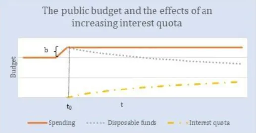
𝑡→∞𝛾𝑝𝑡= 𝜏 + 𝑏 − 𝑧̅ = 𝛾̅ (6)𝑝 In the end, the increasing share of interest payments (5) limits government’s discretionary spending. (6) shows that
due to the interest payments, the limit 𝛾̅𝑝 is always smaller than the initial level of spending 𝛾𝑝0 after having
decided to run a deficit (Figure 2):
Figure 2. The public budget and the effects of an increasing interest quota
With the increasing share of interest payments, the loss due to a politically suboptimal level of spending also increases. Formula (2) shows in combination with formula (6) and (7) that opportunity costs of a default thereby rise with the increasing share of interest payments and the decreasing share of disposable funds. This makes the alternative of defaulting more attractive.
Thus far, we have assumed that the interest rate government must pay on its accumulated debt (𝑖) remains constant.
Based on the market discipline hypothesis, however, we can deduce that with the increasing opportunity costs of a default, financial markets start to worry not to be fully repaid. If they expect a default to become more likely, they react to the unsustainable fiscal policy by selling government bonds. This raises bond yields on secondary markets (Goldstein and Woglom, 1991; Lane, 1993; Capeci, 1994; Bayoumi, Goldstein and Woglom, 1995; Ardagna, Caselli and Lane, 2007).
Bond yields (𝑦) would thereby depend positively on the size of the interest quota (and negatively on the size of disposable
funds for discretionary spending). We formalise this as follows:
𝑦𝐺𝑜𝑣= 𝑟 + (𝜓𝑧)𝜉 𝑤𝑖𝑡ℎ 𝜉 ≥ 1, 𝜓 ≥ 0 (8)
In formula (8), 𝑟 represents the risk-free interest rate and 𝜓 is a coefficient to calibrate the interdependence between
bond yields (𝑦𝐺𝑜𝑣) and the interest quota. We also include a factor 𝜉 to allow for a possible non-linear relationship (Bernoth et al., 2004; Barrios et al., 2009; Delatte et al., 2017).
If the government does not react to rising bond yields on secondary markets by restoring viability, interest rates on primary markets will also rise as a logical consequence when the government rolls over its debt. Debt servicing becomes then more expensive for governments. The initial rise in government bond yields would accelerate the debt servicing problem. Ultimately, this process may result in a self-fulfilling prophecy where market participants’ fear not to be fully repaid results in a default making their fear come true (Calvo, 1988; Cole and Kehoe, 1998; Delatte et al., 2017).
From these considerations, we derive the testing hypothesis, formalised in (7).
Hypothesis: As increasing debt servicing costs make a default relatively more attractive for governments, markets will react to such a development by claiming higher bond yields on secondary markets. Higher interest payments on the accumulated debt thereby lead to higher bond yields on secondary markets.
4. Empirical Testing
In this chapter, I will present the empirical testing of the hypothesis presented above.
4.1 Model Specification
The testing model was formulated as a linear regression.
𝑦𝑖 𝑡= 𝛽0+ 𝛽1𝑒𝑖 𝑡+ 𝛽2𝑋𝑖 𝑡+ 𝜀𝑖 𝑡
In the equation above, 𝑒𝑖,𝑡 represents the interest-related variables, whereas 𝑋𝑖,𝑡is a vector comprising the covariates.
𝜀𝑖,𝑡 is the error term.
In a second step, the model was also tested with time-fixed effects 𝛼𝑡, as it has been suggested by Bernoth et al. (2004).
𝑦𝑖 𝑡= 𝛽0+ 𝛽1𝑒𝑖 𝑡+ 𝛽2𝑋𝑖 𝑡+ 𝜀𝑖 𝑡+ 𝛼𝑡
As an additional feature, different interaction terms had originally been included in the model. They have been excluded again because they did not substantially change coefficients or significance levels.
4.2 Data
Table 1 shows the descriptive statistics for the empirical testing and the sources of the variables. Table 1. Descriptive statistics
Variable Source Obs. Min. Med. Mean Max.
Ten-year government bond yields Eurostat 161 0.09 3.77 3.72 22.50
Interest rate Eurostat, own calculations 167 0.55 3.39 3.29 5.72
Interest quota Eurostat 167 0.10 2.50 2.50 7.30
Interest-revenue quota Eurostat, own calculations 167 0.20 5.70 5.84 16.70
Refinancing conditions Eurostat, own calculations 167 -22.20 0.51 0.81 10.78
Inflation Eurostat 167 -1.7 1.5 1.51 5.50
Foreign assets Eurostat 167 -195.15 -21.66 -34.79 67.67
Public debt Eurostat 167 6.10 70.10 74.93 180.80
Ten-year US-government bond yields Eurostat 167 1.79 2.53 2.73 4.63
EURIBOR Eurostat 167 -0.26 0.57 1.16 4.64
Share of non-performing loans World Bank 148 0.15 4.66 8.06 48.68
For the panel, I chose annual data covering the period from the outbreak of the financial crisis in 2007 up to 2017. It is certainly detrimental to use annual data instead of quarterly data as other studies did. Yet, given that the focus of this analysis lies on the influence of public interest payments on bond yields, there was no other possibility as public budget data are for the most part only published annually. Bernoth et al. (2004) also chose this approach.
For the dependent variable, I selected ten-year government bond yields. As indicated above, they work as a kind of thermometer indicating the daily judgment of financial markets on the health of public finances. Based on our model and the existing empirical literature, we expect that bond yields are higher the higher public interest payments and
subsequently, the higher markets estimate the risk of a default (e. g. Lane, 1993; Ardagna et al., 2007).2
For the key independent variables, I chose four different related variables. This allows us to test to which interest-related variables exactly markets react:
• First, the interest rate the government must pay on its accumulated debt (𝑖, IntRate). As mentioned above, higher
interest payments limit government’s possibilities and thereby make a default more probable. The rising probability of a default would materialise in higher bond yields.
• Second, the interest quota (𝑧, IntQuo). The same logic as for the interest rate applies here: The higher the share
relative to economic output government must pay on its accumulated debt, the higher is the probability of a default due to the rising opportunity costs of a default.
• Third, the interest-growth differential, i. e. the difference between the nominal interest rate government must pay
on its accumulated debt and the nominal growth rate (𝑖 − 𝑔, RefinCon). This differential is derived from the
condition of sustainability of public finances (Blanchard et al., 1990; Barrett, 2018): The lower nominal growth and the higher the interest rate on public debt, the more difficult it becomes for government to keep debt at
sustainable levels. We can expect that this leads to higher bond yields.3
• Fourth and last, the share of public revenues government must dedicate to interest payments (𝑖∗𝐷
𝑇 , IntRevQuo).
Again, the higher the share of revenues government must dedicate to interest payments, the higher the opportunity costs of a default and the higher bond yields.
2 One might argue that there is the problem of endogeneity at hand when regressing bond yields on interest rates on debt.
While bond yields have an influence on future interest rates, the short-term impact is rather negligible. The case of France illustrates this: In 2017, the French public debt amounted to 2.15 trillion Euro. But only roughly 18% were due to be refinanced in less than one year. In the case of a hike in bond yields, the French government would have time to react to this warning sign set by financial markets and adapt its deficit policy to restore viability.
3 A priori, including growth as an independent variable creates the problem of endogeneity due to simultaneity.
Government bond yields have an elementary influence on refinancing conditions of an entire economy. Rising bind yields thereby certainly render businesses’ refinancing more expensive which in turn would impact growth negatively. But in this context, I include growth as part of a differential. The issue of endogeneity is much less severe in this context.
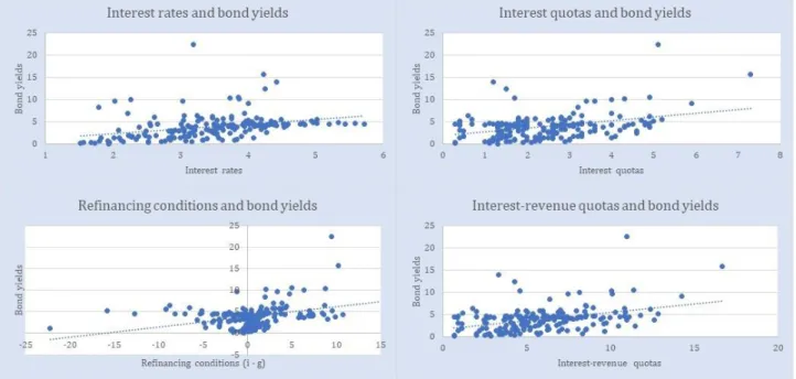
Figure 3. Interest-related independent variables and bond yields
Figure 3 illustrates the univariate regression analyses between the four interest-related independent variables and bond yields as the dependent variable. All four figures are based on the sample employed. In all four cases, the univariate regressions show a correlation justifying the testing method.
I also included several fiscal, macroeconomic and banking variables as covariates based on the empirical literature that
had demonstrated their influence on government bond yields. The variables included were government debt (𝑑, PubDebt)
(e. g. Bernoth et al., 2004; Aßmann and Boysen-Hogrefe, 2012; Ben-Salem and Castelletti, 2017), a square term for public
debt (𝑑², PubDebtSqu) that reflects the non-linear relationship between debt and bond yields (Bernoth et al., 2004; Barrios
et al., 2009; Delatte et al., 2017), the change in public debt (𝛿𝑑𝛿𝑡, ChaPubDebt) to indicate sustainability of public debt, the
absolute size of government debt (𝐷, PubDebtAbs) as a proxy for debt liquidity (Aßmann and Boysen-Hogrefe, 2012),
the inflation rate (𝜋, Infl) (Poghosyan, 2012; Ben-Salem and Castelletti, 2017), the international investment position (ForAss) (Ben-Salem and Castelletti-Font, 2016), US government bond yields (USBondYields) as an indicator for global trends in bond yields, the Euro Interbank Offered Rate (EURIBOR) as an indicator for specific European trends in bond yields, a dummy for the Outright Monetary Transactions Programme (OMT) (the immediate consequence of Mario Draghi’s ‘Whatever it takes’ speech, which had led to a strong downward pressure on yields of the peripheral Eurozone countries), the stock of non-performing loans as a proxy for the health of national banking systems (NPL) and finally a dummy for federal parliamentary elections (Elect).
In the sample, I included all member countries of the Eurozone. Countries having joined EMU later were included since the start of their Eurozone membership. This made the panel unbalanced.
4.3 Empirical Results
The results of the estimations are presented in table 2.
The estimation results show that bond yields are highly correlated with the absolute and relative size of public debt. Bigger and thus more liquid markets for government bond yields entail lower bond yields which lets us conclude that big debtors benefit from a liquidity premium. With the negative sign for public debt and the positive sign for squared public debt and both being significant, previous results are confirmed (Bernoth et al., 2004; Barrios et al., 2009): There is a non-linear effect of the debt quota on bond yields. The annual change in public debt is in contrast only significant in three pooling models. Additionally, the sign switches when refinancing conditions are used as the independent variable.
For inflation, the sign is positive in all four OLS models. Yet, the sign switches in three out of four models from positive to negative when time-fixed effects are employed. Furthermore, the variable is only significant in one model. Foreign assets always show a negative sign and are significant in all models except for one. Given that the size of foreign assets
reflects the competitiveness of an economy, such a result is not surprising (Ben-Salem and Castelletti-Font, 2016). The more competitive an economy is, the higher we can expect the growth rate to be and the easier public debt is to sustain. Table 2. Regression results
Bond yields Intercept 3.01 (1.28)* 4.41 (1.31)*** 2.80 (1.20)* 4.05 (1.29)** PubDebt -0.05 (0.02)** -0.05 (0.02)** -0.07 (0.02)** -0.07 (0.02)** -0.04 (0.01)* -0.04 (0.01)** -0.06 (0.02)** -0-06 (0.02)** PubDebtSqu 0.00 (0.00)*** 0.00 (0.00)*** 0.00 (0.00)*** 0.00 (0.00)*** 0.00 (0.00)*** 0.00 (0.00)*** 0.00 (0.00)*** 0.00 (0.00)*** ChaPubDebt 0.05 (0.02)* 0.03 (0.02) 0.05 (0.02)* 0.03 (0.02) -0.01 (0.02) -0.04 (0.02) 0.05 (0.02)* 0.03 (0.02) IntRate 0.38 (0.25) 0.37 (0.24) IntQuo 0.54 (0.27)* 0.49 (0.26). RefinCon 0.18 (0.05)*** 0.26 (0.05)*** IntRevQuo 0.14 (0.09) 0.13 (0.09) PubDebtAbs -0.00 (0.00). -0.00 (0.00)* -0.00 (0.00). -0.00 (0.00)* -0.00 (0.00)* -0.00 (0.00)** -0.00 (0.00)* -0.00 (0.00)* Infl 0.20 (0.14) -0.13 (0.18) 0.18 (0.14) -0.14 (0.18) 0.47 (0.14)** 0.04 (0.16) 0.21 (0.14) -0.10 (0.18) ForAss -0.61 (0.28)* -0.64 (0.27)* -0.58 (0.28)* -0.63 (0.27)* 0.88 (0.28)** -0.93 (0.26)*** -0.48 (0.31) -0.53 (0.30). USBondYields -0.04 (0.37) -0.05 (0.36) 0.18 (0.34) 0.00 (0.36) EURIBOR -0.02 (0.20) 0.01 (0.20) -0.05 (0.19) 0.03 (0.20) OMT -2.28 (0.42)*** -2.25 (0.41)*** -1.99 (0.41)*** -2.27 (0.42)*** NPL 0.05 (0.02)* 0.03 (0.02)* 0.05 (0.02)* 0.04 (0.02) 0.05 (0.02)* 0.02 (0.02) 0.05 (0.02)* 0.03 (0.02) Elect 0.42 (0.30) 0.33 (0.29) 0.43 (0.29) 0.34 (0.29) 0.41 (0.28) 0.33 (0.27) 0.43 (0.30) 0.34 (0.29)
Time-FE No Yes No Yes No Yes No Yes
N 142 142 142 142 142 142 142 142
Adj. R² 0.70 0.64 0.71 0.64 0.73 0.69 0.70 0.64
Standard errors in parentheses; ‘.’: 10% significance level, ‘*’: 5%, ‘**’: 1%, ‘***’: 0.1%
The size of non-performing loans has a significant impact on government bond yields in the OLS models. The effect vastly disappears when time-fixed effects are included. There is thereby some evidence for the vicious sovereign bank-nexus (Acharya et al., 2014).
US-American bond yields and the EURIBOR show no significant correlation with bond yields whatsoever. The same is true for the election dummy. The reason for this might be that for the elections covered by the sample there was no risk-premium on covered bonds due to political uncertainty.
Although all four interest-related variables show a positive sign, only two are significant: the interest quota and the interest rate-growth differential. With the sign being positive as predicted by the theoretical model presented above, there is evidence for markets reacting to high public interest payments. A one percent increase in the interest quota leads to an increase of 0.54 percentage points in bond yields (0.49 for the time-fixed effects model), an increase of one point in the interest-growth differential in turn leads to an increase of 0.18 percentage points (0.26 for the time-fixed effects model). These findings confirm the theoretical considerations.
4.4 Model Diagnostics and Robustness Check
Table 3. F-test results
Models IntRate Models IntQuo Models RefinCon Models IntRevQuo
F = 2.88 p = 0.01 F = 2.78 p = 0.01 F = 4.22 p = 0.00 F = 2.82 p = 0.01
For the model diagnostics, the F-test is significant for all four models (see table 3). The use of time-fixed effects is thereby appropriate. Yet, the results presented in the section above are vastly robust to both testing methods. Particularly, there are no conflicting results concerning the four interest-related variables. The same applies to the covariates.
Table 4 indicates the results of the robustness checks with M-estimators. The coefficients for the independent variables vastly confirm the results of the OLS regressions and those with time fixed-effects. In particular the four interest-related variables show the same positive algebraic sign.
Table 4. Robustness check with M-estimators
Bond yields Intercept 0.26 (0.62) 1.46 (0.65) 1.34 (0.61) 1.34 (0.61) PubDebt -0.03 (0.01) -0.05 (0.01) -0.04 (0.01) -0.04 (0.01) PubDebtSqu 0.00 (0.00) 0.00 (0.00) 0.00 (0.00) 0.00 (0.00) ChaPubDebt 0.10 (0.01) 0.10 (0.01) 0.10 (0.01) 0.10 (0.01) IntRate 0.37 (0.12) IntQuo 0.32 (0.13) RefinCon 0.06 (0.02) IntRevQuo 0.12 (0.04) PubDebtAbs -0.00 (0.00) -0.00 (0.00) -0.00 (0.00) -0.00 (0.00) Infl 0.34 (0.07) 0.34 (0.07) 0.43 (0.07) 0.34 (0.07) ForAss -0.41 (0.14) -0.46 (0.14) -0.51 (0.13) -0.36 (0.14) USBondYields 0.64 (0.18) 0.64 (0.18) 0.70 (0.17) 0.66 (0.17) EURIBOR -0.15 (0.10) -0.11 (0.10) -0.10 (0.09) -0.10 (0.10) OMT -1.01 (0.20) -1.07 (0.21) -1.07 (0.20) -1.05 (0.20) NPL 0.07 (0.01) 0.07 (0.01) 0.07 (0.01) 0.07 (0.01) Elect 0.04 (0.14) 0.07 (0.15) 0.11 (0.14) 0.08 (0.14)
5. Conclusion
This paper has analysed the interplay between governments’ interest payments on the accumulated debt and government bond yields on secondary markets. From a theoretical point of view, increasing interest payments limit the government’s fiscal possibilities. This raises the opportunity costs of a default which thereby becomes more probable. In such a situation, markets start to worry about not being fully repaid and raise the risk premia on secondary markets. Increasing interest payments thereby fuel bond yields on secondary markets. At a later stage increasing bond yields could translate into higher refinancing costs on primary markets. This could then ultimately lead to a self-fulfilling prophecy.
The empirical analysis based on data for the Eurozone from 2007 to 2017 confirms the theoretical model when it comes to interest quotas and refinancing conditions. High public interest payments and deteriorating financing conditions thereby had an impact on rising bond yields during the Euro crisis. This is not the case, though, for the interest rate and the interest-revenue quota.
Governments with already high debt thereby face the danger that their already high interest payments lead to further rising refinancing costs, first on secondary markets and later potentially also on primary markets. The policy lesson which can be drawn from these results is that governments should bother to keep public debt and with it interest payments under control so that market participants do not doubt the government’s commitment to honour its debt obligations. Otherwise, governments could quickly find themselves in a vicious circle of high interest payments and increasing future interest payments, which would make a default more probable.
References
Acharya, V., Drechsler, I., & Schnabl, P. (2014). A Pyrrhic Victory? Bank Bailouts and Sovereign Credit Risk. The Journal of Finance, 69(6), 2689-2739.https://doi.org/10.1111/jofi.12206
Afonso, A., Arghyrou, M. G., & Kontonikas, A. (2015). The determinants of sovereign bond yield spreads in EMU. ECB
Working Paper, 1781.
Alichi, A. (2008). A Model of Sovereign Debt in Democracies. IMF Working Paper, WP/08/152.
https://doi.org/10.5089/9781451870107.001
Ardagna, S., Caselli, F., & Lane, T. (2007). Fiscal Discipline and the Cost of Public Debt Service: Some Estimates for
OECD Countries. The B.E. Journal of Macroeconomics,7(1), 1-33.https://doi.org/10.2202/1935-1690.1417
Aßmann, C., & Boysen-Hogrefe, J. (2012). Determinants of government bond spreads in the Euro Area: in good times as
in bad. Empirica, 39(3), 341-356. https://doi.org/10.1007/s10663-011-9171-6
Attinasi, M. G., Checherita-Westphal, C., & Nickel, C. (2009). What explains the surge in euro area sovereign spreads
during the financial crisis of 2007-09? ECB Working Paper, No.1131.
Barrett, P. (2018). Interest-Growth Differentials and Debt Limits in Advanced Economies. IMF Working Paper,
WP/18/82. https://doi.org/10.5089/9781484350980.001
Barrios, S., Iversen, P., Lewandowska, M., & Setzer, R. (2009). Determinants of intra-euro area government bond spreads
during the financial crisis. Economic Papers,388, November 2009.
Bayoumi, T., Goldstein, M., & Woglom, G. (1995). Do Credit markets discipline sovereign borrowers? Evidence from
U. S. states. Journal of Money Credit, and Banking, 27, 1046–1059.https://doi.org/10.2307/2077788
Ben-Salem, M., & Castelletti-Font, B. (2016). Which combination of of fiscal and external imbalances to determine the
long-run dynamics of sovereign bond yields? Banque de France document de travail No. 606.
Bernoth, K., Von-Hagen, J., & Schuknecht, L. (2004). Sovereign risk premia in the European government bond market.
ECB Working Paper, 369.
Blanchard, O., Chouraqui, J. C., Hagemann, R. P., & Sartor, N. (1990). The Sustainability of Fiscal Policy: New Answers
to an Old Question. OECD Economic Studies, No.15.
Borensztein, E., & Panizza, U. (2008). The Costs of a Sovereign Default. IMF Working Paper, WP/08/238.
https://doi.org/10.5089/9781451870961.001
Buiter, W. H., & Rahbari, E. (2013). Why Do Governments Default, and Why Don’t They Default More Often? CEPR
Discussion Paper, DP9492.
Calvo, G. (1988). Servicing the Public Debt: The Role of Expectations. American Economic Review,78(4), 647-661.
Capeci, J. (1994). Local fiscal policies, default risk, and municipal borrowing costs. Journal of Public Economics, 53,
Cole, H. L., & Kehoe, T. J. (1998). Self-Fulfilling Debt Crises. Federal Reserve Bank of Minneapolis Research Department Staff Report 211.
De-Grauwe, P., & Yuemei, J. (2013). Self-fulfilling crises in the Eurozone: An empirical test. Journal of International
Money and Finance,34, 15-36.https://doi.org/10.1016/j.jimonfin.2012.11.003
Delatte, A. L., Fouquau, J., & Portes, R. (2017). Regime-Dependent Sovereign Risk Pricing During the Euro Crisis.
Review of Finance, 21(1), 363–385.
Domar, E. (1944). The “Burden of the Debt” and National Income. The American Economic Review,34(4), 798-827.
Downs, A. (1957). An Economic Theory of Democracy. New York: Harper and Row.
Fratzscher, M., & Ehrmann, M. (2015). Euro Area Government Bonds: Integration and Fragmentation During the
Sovereign Bond Crisis. DIW Berlin Discussion Paper, No.1479.
Gerlach, S., Schulz, A., & Wolff, G. B. (2010). Banking and sovereign risk in the euro area. Bundesbank discussion paper
series 1. Economic Studies, No.09/2010.
Goldstein, M., & Woglom, T. (1995). Market-Based Fiscal Discipline in Monetary Unions: Evidence from the U.S.
Municipal Bond Market. IMF Working Paper 1991/89.https://doi.org/10.5089/9781451851205.001
Lane, T. D. (1993). Market Discipline. IMF (ed.). IMF Staff Papers, 40(1) (pp. 53-88). https://doi.org/10.2307/3867377
Pelizzon, L., Subrahmanyam, M. G., Tomio, D., & Uno, J. (2016). Sovereign credit risk, liquidity and the European
Central Bank intervention: Deus ex machina? Journal of Financial Economics, 122(1), 86-115.
https://doi.org/10.1016/j.jfineco.2016.06.001
Poghosyan, T. (2014). Long-Run and Short-Run Determinants of Sovereign Bond Yields in Advanced Economies.
Economic Systems,38(1), 100-114.https://doi.org/10.1016/j.ecosys.2013.07.008
Reinhart, C. M., & Rogoff, K. S. (2009). This Time Is Different: Eight Centuries of Financial Folly. Princeton: Princeton
University Press.
Copyrights
Copyright for this article is retained by the author(s), with first publication rights granted to the journal.
This is an open-access article distributed under the terms and conditions of the Creative Commons Attribution license which permits unrestricted use, distribution, and reproduction in any medium, provided the original work is properly cited.