Large dimensional analysis and optimization of robust
shrinkage covariance matrix estimators
Romain Couillet, Matthew Mckay
To cite this version:
Romain Couillet, Matthew Mckay.
Large dimensional analysis and optimization of robust
shrinkage covariance matrix estimators. Journal of Multivariate Analysis, Elsevier, 2014, 131,
pp.99 - 120.
<10.1016/j.jmva.2014.06.018>.
<hal-01098854>
HAL Id: hal-01098854
https://hal.archives-ouvertes.fr/hal-01098854
Submitted on 29 Dec 2014
HAL
is a multi-disciplinary open access
archive for the deposit and dissemination of
sci-entific research documents, whether they are
pub-lished or not.
The documents may come from
teaching and research institutions in France or
abroad, or from public or private research centers.
L’archive ouverte pluridisciplinaire
HAL
, est
destin´
ee au d´
epˆ
ot et `
a la diffusion de documents
scientifiques de niveau recherche, publi´
es ou non,
´
emanant des ´
etablissements d’enseignement et de
recherche fran¸
cais ou ´
etrangers, des laboratoires
publics ou priv´
es.
Large Dimensional Analysis and Optimization of
Robust Shrinkage Covariance Matrix Estimators
✩Romain Couilleta, Matthew McKayb
aTelecommunication department, Sup´elec, Gif sur Yvette, France b
Hong Kong University of Science and Technology
Abstract
This article studies two regularized robust estimators of scatter matrices pro-posed in parallel in (Chen et al., 2011) and (Pascal et al., 2013), based on Tyler’s robust M-estimator (Tyler, 1987) and on Ledoit and Wolf’s shrinkage covariance matrix estimator (Ledoit and Wolf, 2004). These hybrid estimators have the advantage of conveying (i) robustness to outliers or impulsive samples and (ii) small sample size adequacy to the classical sample covariance matrix estimator. We consider here the case of i.i.d. elliptical zero mean samples in the regime where both sample and population sizes are large. We demonstrate that, under this setting, the estimators under study asymptotically behave similar to well-understood random matrix models. This characterization allows us to derive optimal shrinkage strategies to estimate the population scatter matrix, improv-ing significantly upon the empirical shrinkage method proposed in (Chen et al., 2011).
Keywords: random matrix theory, robust estimation, linear shrinkage.
1. Introduction
Many scientific domains customarily deal with (possibly small) sets of large dimensional data samples from which statistical inference is performed. This is in particular the case in financial data analysis where few stationary monthly observations of numerous stock indexes are used to estimate the joint covariance matrix of the stock returns (Laloux et al., 2000; Ledoit and Wolf, 2003; Rubio et al., 2012), bioinformatics where clustering of genes is obtained based on gene sequences sampled from a small population (Sch¨afer and Strimmer, 2005), com-putational immunology where correlations among mutations in viral strains are estimated from sampled viral sequences and used as a basis of novel vaccine design (Dahirel et al., 2011; Quadeer et al., 2013), psychology where the covari-ance matrix of multiple psychological traits is estimated from data collected on
✩Couillet’s work is supported by the ERC MORE EC–120133.
Email addresses: [email protected](Romain Couillet),[email protected]
a group of tested individuals (Steiger, 1980), or electrical engineering at large where signal samples extracted from a possibly short time window are used to retrieve parameters of the signal (Scharf, 1991). In many such cases, the num-bern of independent data samplesx1, . . . , xn ∈CN (orRN) may not be large
compared to the sizeN of the population, suggesting that the empirical sample covariance matrix ¯CN =n1Pni=1(xi−x¯)(xi−x¯)∗, ¯x=n1Pni=1xi, is a poor
es-timate forCN = E[(x1−x¯)(x1−x¯)∗]. Several solutions have been proposed to work around this problem. If the end application is not to retrieveCN but some
metric of it, recent works on random matrix theory showed that replacingCN in
the metric by ¯CN often leads to a biased estimate of the metric (Mestre, 2008b),
but that this estimate can be corrected by an improved estimation of the metric itself via the samplesx1, . . . , xn (Mestre, 2008a). However, when the object
un-der interest isCN itself andN ≃n, there is little hope to retrieve any consistent
estimate ofCN. A popular alternative proposed originally in (Ledoit and Wolf,
2004) is to “shrink” ¯CN, i.e., consider instead ¯CN(ρ) = (1−ρ) ¯CN+ρIN for an
appropriateρ∈[0,1] that minimizes the average distance E[tr( ¯CN(ρ)−CN)2].
The interest of ρ here is to give more or less weight to ¯CN depending on the
relevance of thensamples, so that in particularρis better chosen close to zero whennis large and close to one whennis small.
In addition to the problem of scarcity of samples, it is often the case that outliers are present among the set of samples. These outliers may arise from erroneous or inconsistent data (e.g., individuals under psychological or biolog-ical tests incorrectly identified to fit the test pattern), or from the corruption of some samples by external events (e.g., interference by ambient electromag-netic noise in signal processing). These outliers, if not correctly handled, may further corrupt the statistical inference and in particular the estimation ofCN.
The field of robust estimation intends to deal with this problem (Huber, 1981; Maronna et al., 2006) by proposing estimators that have the joint capability to naturally attenuate the effect of outliers (Huber, 1964) as well as to appro-priately handle samples of an impulsive nature (Tyler, 1987), e.g., elliptically distributed data. A common denominator of such estimators is their belong-ing to the class of M-estimators, therefore takbelong-ing the form of the solution to an implicit equation. This poses important problems of analysis in smallN, n
dimensions, resulting mostly in only asymptotic results in the regime N fixed and n→ ∞ (Maronna, 1976; Kent and Tyler, 1991). This regime is however inconsistent with the present scenario of scarce data whereN ≃n. Nonethe-less, recent works based on random matrix theory have shown that a certain family of such robust covariance matrix estimators asymptotically behave as
N, n→ ∞ and N/n→c ∈(0,∞) similar to classical random matrices taking (almost) explicit forms. Such observations were made for the class of Maronna’s M-estimators of scatter (Maronna, 1976) for sample vectors whose independent entries can contain outliers (Couillet et al., 2013a) and for elliptically distributed samples (Couillet et al., 2013b), as well as for Tyler’s M-estimator (Tyler, 1987) in (Zhang et al., 2014).
In this article, we study two hybrid robust shrinkage covariance matrix esti-mates ˆCN(ρ) (hereafter referred to as the Pascal estimate) and ˇCN(ρ) (hereafter
referred to as the Chen estimate) proposed in parallel in (Pascal et al., 2013) and in (Chen et al., 2011), respectively. Both matrices, whose definition is introduced in Section 2 below, are empirically built upon Tyler’s M-estimate (Tyler, 1987) originally designed to cope with elliptical samples whose distri-bution is unknown to the experimenter and upon the Ledoit–Wolf shrinkage estimator (Ledoit and Wolf, 2004). In (Pascal et al., 2013) and (Chen et al., 2011), ˆCN(ρ) and ˇCN(ρ) were proved to be well-defined as the unique
solu-tions to their defining fixed-point matrices. However, little is known of their performance as estimators ofCN in the regimeN ≃n of interest here. Some
progress in this direction was made in (Chen et al., 2011) but this work does not manage to solve the optimal shrinkage problem consisting of findingρsuch that E[tr( ˇCN(ρ)−CN)2] is minimized and resorts to solving an approximate
problem instead.
The present article studies the matrices ˆCN(ρ) and ˇCN(ρ) from a random
matrix approach, i.e., in the regime whereN, n→ ∞with N/n→c ∈(0,∞), and under the assumption of the absence of outliers. Our main results are as follows:
• we show that, under the aforementioned setting, both ˆCN(ρ) and ˇCN(ρ)
asymptotically behave similar to well-known random matrix models and prove in particular that both have a well-identified limiting spectral dis-tribution;
• we prove that, up to a change in the variable ρ, the matrices ˇCN(ρ) and
ˆ
CN(ρ)/(N1 tr ˆCN(ρ)) are essentially the same forN, nlarge, implying that
both achieve the same optimal shrinkage performance;
• we determine the optimal shrinkage parameters ˆρ⋆ and ˇρ⋆ that
mini-mize the almost sure limits limN N1 tr( ˆCN(ρ)/(N1 tr ˆCN(ρ))−CN)2 and
limN N1 tr( ˇCN(ρ)−CN)2, respectively, both limits being the same. We
then propose consistent estimates ˆρN and ˇρN for ˆρ⋆and ˇρ⋆ which achieve
the same limiting performance. We finally show by simulations that a sig-nificant gain is obtained using ˆρ⋆(or ˆρ
N) and ˇρ⋆(or ˇρN) compared to the
solution ˇρO of the approximate problem developed in (Chen et al., 2011).
In practice, these results allow for a proper use of ˆCN(ρ) and ˇCN(ρ) in
antici-pation of the absence of outliers. In the presence of outliers, it is then expected that both Pascal and Chen estimates will exhibit robustness properties that their asymptotic random matrix equivalents will not. Note in particular that, although ˆCN(ρ) and ˇCN(ρ) are shown to be asymptotically equivalent in the
absence of outliers, it is not clear at this point whether one of the two estimates will show better performance in the presence of outliers. The study of this interesting scenario is left to future work.
The remainder of the article is structured as follows. In Section 2, we in-troduce our main results on the largeN, nbehavior of the matrices ˆCN(ρ) and
ˇ
CN(ρ). In Section 3, we develop the optimal shrinkage analysis, providing in
remarks are provided in Section 4. All proofs of the results of Section 2 and Section 3 are then presented in Section 5.
General notations: The superscript (·)∗ stands for Hermitian transpose in
the complex case or transpose in the real case. The notation k · k stands for the spectral norm for matrices and the Euclidean norm for vectors. The Dirac measure at point xis denotedδx. The ordered eigenvalues of a Hermitian (or
symmetric) matrixXof sizeN×Nare denotedλ1(X)≤. . .≤λN(X). Forℓ >0
and a positive and positively supported measureν, we define Mν,ℓ=R tℓν(dt)
(may be infinite). The arrow “−→a.s.” designates almost sure convergence.
2. Main results
We start by introducing the main assumptions of the data model under study. We consider n samples vectors x1, . . . , xn ∈ CN (or RN) having the
following characteristics.
Assumption 1 (Growth rate). Denoting cN = N/n, cN → c ∈ (0,∞) as
N→ ∞.
Assumption 2 (Population model). The vectorsx1, . . . , xn ∈CN (or RN)
are independent with
a. xi = √τiANyi, where yi ∈ CN¯ (or RN¯), N¯ ≥ N, is a random zero
mean unitarily (or orthogonally) invariant vector with norm kyik2 = ¯N,
AN ∈ CN×N¯ is deterministic, and τ1, . . . , τn is a collection of positive
scalars. We shall denotezi=ANyi.
b. CN ,ANAN∗ is nonnegative definite, with trace N1 trCN = 1and spectral
norm satisfyinglim supNkCNk<∞;
c. νN , N1 PNi=1δλi(CN) satisfies νN →ν weakly with ν 6=δ0 almost
every-where.
Since all considerations to come are equally valid overCor R, we will
con-sider by default thatx1, . . . , xn ∈CN. As the analysis will show, the positive
scalars τi have no impact on the robust covariance estimates; with this
defini-tion, the distribution of the vectorsxicontains in particular the class of elliptical
distributions. Note that the assumption thatyiis zero mean unitarily invariant
with norm ¯N is equivalent to saying thatyi =
√¯
Nk˜yi˜yik with ˜yi∈C
¯
N standard
Gaussian. This, along withAN ∈ CN×N¯ and lim supNkCNk <∞, implies in
particular thatkxik2is of order N. The assumption thatν 6=δ0almost every-where avoids the degenerate scenario every-where an overwhelming majority of the eigenvalues of CN tend to zero, whose practical interest is quite limited.
Fi-nally note that the constraint 1
N trCN = 1 is inconsequential and in fact defines
uniquely both terms in the productτiCN.
The following two theorems introduce the robust shrinkage estimators ˆCN(ρ)
Theorem 1 (Pascal Estimate). Let Assumptions 1 and 2 hold. For ε ∈
(0,min{1, c−1}), defineRˆ
ε= [ε+ max{0,1−c−1},1]. For eachρ∈(max{0,1−
c−N1},1], letCˆN(ρ) be the unique solution to
ˆ CN(ρ) = (1−ρ) 1 n n X i=1 xix∗i 1 Nx ∗ iCˆN(ρ)−1xi +ρIN. Then, asN → ∞, sup ρ∈Rˆε CˆN(ρ)−SˆN(ρ) a.s. −→0 where ˆ SN(ρ) = 1 ˆ γ(ρ) 1−ρ 1−(1−ρ)c 1 n n X i=1 ziz∗i +ρIN
andˆγ(ρ)is the unique positive solution to the equation inγˆ 1 =
Z t
ˆ
γρ+ (1−ρ)tν(dt).
Moreover, the functionρ7→ˆγ(ρ)thus defined is continuous on(0,1]. Proof. The proof is deferred to Section 5.1.
Theorem 2 (Chen Estimate). Let Assumptions 1 and 2 hold. Forε∈(0,1), defineRˇε= [ε,1]. For eachρ∈(0,1], letCˇN(ρ)be the unique solution to
ˇ CN(ρ) = ˇ BN(ρ) 1 N tr ˇBN(ρ) where ˇ BN(ρ) = (1−ρ)1 n n X i=1 xix∗i 1 Nx∗iCˇN(ρ)−1xi +ρIN. Then, asN → ∞, sup ρ∈Rˇε CˇN(ρ)−SˇN(ρ) a.s. −→0 where ˇ SN(ρ) = 1−ρ 1−ρ+Tρ 1 n n X i=1 zizi∗+ Tρ 1−ρ+TρIN
in whichTρ=ργˇ(ρ)F(ˇγ(ρ);ρ)with, for allx >0,
F(x;ρ) = 1 2(ρ−c(1−ρ)) + r 1 4(ρ−c(1−ρ)) 2 + (1−ρ)1 x
andˇγ(ρ)is the unique positive solution to the equation inγˇ 1 =
Z t
ˇ
γρ+(1−ρ)1c−+ρF(ˇγ;ρ)tν(dt).
Moreover, the functionρ7→ˇγ(ρ)thus defined is continuous on(0,1]. Proof. The proof is deferred to Section 5.2.
Theorem 1 and Theorem 2 show that, as N, n → ∞ with N/n → c, the matrices ˆCN(ρ) and ˇCN(ρ), defined as the non-trivial solution of fixed-point
equations, behave similar to matrices ˆSN(ρ) and ˇSN(ρ), respectively, whose
characterization is well-known and much simpler than that of ˆCN(ρ) and ˇCN(ρ)
themselves. Indeed, ˆSN(ρ) and ˇSN(ρ) are random matrices of the sample
co-variance matrix type thoroughly studied in e.g., (Mar˘cenko and Pastur, 1967; Silverstein and Bai, 1995; Silverstein and Choi, 1995).
As a side remark, it is shown in (Pascal et al., 2013) that for eachN, nfixed withn≥N+ 1, ˆCN(ρ)→CˆN(0) asρ→0 with ˆCN(0) defined (almost surely)
as one of the (uncountably many) solutions to ˆ CN(0) = 1 n n X i=1 xix∗i 1 Nx ∗ iCˆN(0)−1xi . (1)
In the regime whereN, n→ ∞andN/n→c, this result is difficult to generalize as it is challenging to handle the limit kCˆN(ρN)−SˆN(ρN)k for a sequence
{ρN}∞N=1 with ρN → 0. The requirement that ρN → ρ0 > 0 on any such sequence is indeed at the core of the proof of Theorem 1 (see Equations (5) and (6) in Section 5.1 whereρ0 >0 is necessary to ensure e+ <1). This explains why the set ˆRεin Theorem 1 excludes the region [0, ε). Similar arguments hold
for ˇCN(ρ). As a matter of fact, the behavior of any solution ˆCN(0) to (1) in the
largeN, nregime, recently derived in (Zhang et al., 2014), remains difficult to handle with our proof technique.
An immediate consequence of Theorem 1 and Theorem 2 is that the empirical spectral distributions of ˆCN(ρ) and ˇCN(ρ) converge to the well-known respective
limiting distributions of ˆSN(ρ) and ˇSN(ρ), characterized in the following result.
Corollary 1 (Limiting spectral distribution). Under the settings of The-orem 1 and TheThe-orem 2,
1 N N X i=1 δ λi( ˆCN(ρ)) a.s. −→µˆρ, ρ∈Rˆε 1 N N X i=1 δ λi( ˇCN(ρ)) a.s. −→µˇρ, ρ∈Rˇε
where the convergence arrow is understood as the weak convergence of probability measures, for almost every sequence{x1, . . . , xn}∞n=1, and where
ˆ µρ = max{0,1−c−1}δρ+ ˆµρ ˇ µρ = max{0,1−c−1}δ Tρ 1−ρ+Tρ + ˇµρ
withµˆρ andµˇρ continuous finite measures with compact support in [ρ,∞) and
[Tρ(1−ρ+Tρ)−1,∞)respectively, real analytic wherever their density is positive.
The measureµˆρis the only measure with Stieltjes transformmµρˆ (z)defined, for
z∈Cwithℑ[z]>0, as mµρˆ (z) = ˆγ 1−(1−ρ)c 1−ρ Z 1 ˆ z(ρ) +1+ctδˆ(z) ν(dt)
wherezˆ(ρ) = (ρ−z)ˆγ(ρ)1−(11−−ρρ)c and ˆδ(z) is the unique solution with positive imaginary part of the equation inδˆ
ˆ δ= Z t ˆ z(ρ) +1+tcδˆ ν(dt).
The measureµˇρis the only measure with Stieltjes transformmµˇρ(z)defined, for
ℑ[z]>0 as mµρˇ (z) = 1−ρ+Tρ 1−ρ Z 1 ˇ z(ρ) + t 1+cˇδ(z) ν(dt) withzˇ(ρ) = 1
1−ρTρ(1−z)−zandδˇ(z)the unique solution with positive imaginary
part of the equation inδˇ
ˇ δ= Z t ˇ z(ρ) +1+tcδˇ ν(dt).
Proof. This is an immediate application of (Silverstein and Bai, 1995;
Silver-stein and Choi, 1995) and Theorems 1 and 2.
From Corollary 1, ˆµρ is continuous on (ρ,∞) so that ˆµρ(dx) = ˆpρ(x)dx
where, from the inverse Stieltjes transform formula (see e.g., (Bai and Silver-stein, 2009)) for allx∈(ρ,∞),
ˆ pρ(x) = lim ε→0 1 πℑ mµρˆ (x+ıε).
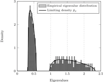
Lettingε >0 small and approximating ˆpρ(x) by π1ℑ[mµρˆ (x+ıε)] allows one to depict ˆpρ approximately. Similarly, ˇµρ(dx) = ˇpρ(x)dx for allx∈ (Tρ(1−ρ+
Tρ)−1,∞) which can be obtained equivalently. This is performed in Figure 1
0 1 2 3 4 0 0.5 1 1.5 Eigenvalues D en si ty
Empirical eigenvalue distribution Limiting density ˆpρ
Figure 1: Histogram of the eigenvalues of ˆCN (Pascal type) forn= 2048,N = 256,CN =
1
3diag(I128,5I128),ρ= 0.2, versus limiting eigenvalue distribution.
0 0.5 1 1.5 2 2.5 0 1 2 3 Eigenvalues D en si ty
Empirical eigenvalue distribution Limiting density ˇpρ
Figure 2: Histogram of the eigenvalues of ˇCN (Chen type) forn= 2048,N = 256,CN =
1
3diag(I128,5I128),ρ= 0.2, versus limiting eigenvalue distribution.
forρ = 0.2, N = 256, n= 2048, CN = diag(I128,5I128), versus their limiting distributions for c = 1/8. Figure 3 depicts ˇCN(ρ) for ρ = 0.8, N = 1024,
n= 512,CN = diag(I128,5I128) versus its limiting distribution for c= 2. Note that, whenc= 1/8, the eigenvalues of ˇCN(ρ) concentrate in two bulks close to
1 1.5 2 2.5 0 0.2 0.4 0.6 0.8 1 1.2 Eigenvalues D en si ty
Empirical eigenvalue distribution Limiting density ˇpρ
Dirac mass 1/2
Figure 3: Histogram of the eigenvalues of ˇCN (Chen type) forn= 512,N = 1024,CN =
1
3diag(I128,5I128),ρ= 0.8, versus limiting eigenvalue distribution.
the same reasoning holds up to a multiplicative constant. However, whenc= 2, the eigenvalues of ˇCN(ρ) are quite remote from masses in 1/3 and 5/3, an
observation known since (Mar˘cenko and Pastur, 1967).
Another corollary of Theorem 1 and Theorem 2 is the joint convergence (over bothρand the eigenvalue index) of the individual eigenvalues of ˆCN(ρ) to those
of ˆSN(ρ) and of the individual eigenvalues of ˇCN(ρ) to those of ˇSN(ρ), as well as
the joint convergence overρof the moments of the empirical spectral distribu-tions of ˆCN(ρ) and ˇCN(ρ). These joint convergence properties are fundamental
in problems of optimization of the parameterρas discussed in Section 3.
Corollary 2 (Joint convergence properties). Under the settings of Theo-rem 1 and TheoTheo-rem 2,
sup ρ∈Rˆε max 1≤i≤n λi( ˆCN(ρ))−λi( ˆSN(ρ)) a.s. −→0 sup ρ∈Rˇε max 1≤i≤n λi( ˇCN(ρ))−λi( ˇSN(ρ)) a.s. −→0.
This result implies
lim sup N sup ρ∈Rˆε kCˆN(ρ)k<∞ lim sup N sup ρ∈Rˇε kCˇN(ρ)k<∞.
that, for eachℓ∈N, sup ρ∈Rˆε 1 N tr ˆCN(ρ) ℓ −Mµρ,ℓˆ a.s. −→0 sup ρ∈Rˇε 1 N tr ˇCN(ρ) ℓ−M ˇ µρ,ℓ a.s. −→0
where, in particular,Mµρˆ ,1= ˆγ(1ρ)1−1(1−−ρρ)c+ρandMµρ,ˇ 1= 1.
Proof. The proof is provided in Section 5.3.
3. Application to optimal shrinkage
We now apply Theorems 1 and 2 to the problem of optimal linear shrinkage, originally considered in (Ledoit and Wolf, 2004) for the simpler sample covari-ance matrix model. The optimal linear shrinkage problem consists in choosing
ρto be such that a certain distance measure between ˆCN(ρ) (or ˇCN(ρ)) andCN
is minimized, therefore allowing for a more appropriate estimation of CN via
ˆ
CN(ρ) or ˇCN(ρ). In (Chen et al., 2011), the authors studied this problem in the
specific case of ˇCN(ρ) but did not find an expression for the optimal theoretical
ρdue to the involved structure of ˇCN(ρ) for all finiteN, nand therefore resorted
to solving an approximate problem, the solution of which is denoted here ˇρO.
Instead, we show that for largeN, nvalues the optimalρunder study converges to a limiting value ˇρ⋆ that takes an extremely simple explicit expression and a similar result holds for ˆCN(ρ) for which an equivalent optimal ˆρ⋆is defined.
Our first result is a lemma of fundamental importance which demonstrates that, up to a change in the variableρ, ˆSN(ρ)/Mµρ,ˆ 1and ˇSN(ρ) (constructed from
the samplesx1, . . . , xn) are completely equivalent to the original Ledoit–Wolf
linear shrinkage model for the (non observable) samplesz1, . . . , zn.
Lemma 1 (Asymptotic Model Equivalence). For eachρ∈(0,1], there ex-ist uniqueρˆ∈(max{0,1−c−1},1]andρˇ∈(0,1]such that
ˆ SN(ˆρ) Mµˆρ,ˆ1 = ˇSN(ˇρ) = (1−ρ)1 n n X i=1 ziz∗i +ρIN.
Besides, the maps(0,1]→(max{0,1−c−1},1],ρ7→ρˆand(0,1]→(0,1],ρ7→ρˇ
thus defined are continuously increasing and onto. Proof. The proof is provided in Section 5.4.
Thanks to Lemma 1, we now show that the optimal shrinkage parameters
ρ for both ˆCN(ρ)/(N1 tr ˆCN(ρ)) and ˇCN(ρ) lead to the same asymptotic
per-formance, which corresponds to the asymptotically optimal Ledoit–Wolf linear shrinkage performance but for the vectorsz1, . . . , zn.
Proposition 1 (Optimal Shrinkage). For each ρ∈(0,1], define1 ˆ DN(ρ) = 1 Ntr ˆ CN(ρ) 1 N tr ˆCN(ρ) −CN !2 ˇ DN(ρ) = 1 Ntr ˇCN(ρ)−CN 2 . Also denote D⋆ = c Mν,2−1 c+Mν,2−1, ρ ⋆ = c c+Mν,2−1, and ρˆ ⋆ ∈ (max{0,1−c−1},1], ˇ
ρ⋆∈(0,1]the unique solutions to
ˆ ρ⋆ 1 ˆ γ( ˆρ⋆) 1−ρˆ⋆ 1−(1−ρˆ⋆)c + ˆρ⋆ = Tρˇ⋆ 1−ρˇ⋆+T ˇ ρ⋆ =ρ ⋆.
Then, lettingε <min(ˆρ⋆−max{0,1−c−1},ρˇ⋆), under the setting of Theorem 1 and Theorem 2, inf ρ∈Rˆε ˆ DN(ρ)−→a.s. D⋆, inf ρ∈Rˇε ˇ DN(ρ)−→a.s. D⋆ and ˆ DN(ˆρ⋆) a.s. −→D⋆, DˇN(ˇρ⋆) a.s. −→D⋆.
Moreover, letting ρˆN and ρˇN be random variables such that ρˆN
a.s. −→ ρˆ⋆ and ˇ ρN a.s. −→ρˇ⋆, ˆ DN(ˆρN)−→a.s. D⋆, DˇN(ˇρN)−→a.s. D⋆.
Proof. The proof is provided in Section 5.5.
The last part of Proposition 1 states that, if consistent estimates ˆρN and
ˇ
ρN of ˆρ⋆ and ˇρ⋆ exist, then they have optimal shrinkage performance in the
largeN, nlimit. Such estimates may of course be defined in multiple ways. We present below a simple example based on ˆCN(ρ) and ˇCN(ρ).
Proposition 2 (Optimal Shrinkage Estimate). Under the setting of Propo-sition 1, letρˆN ∈(max{0,1−c−1},1] andρˇN ∈(0,1] be solutions (not
neces-sarily unique) to ˆ ρN 1 N tr ˆCN(ˆρN) = cN 1 N tr 1 n Pn i=1 xix∗ i 1 Nkxik2 2 −1 ˇ ρNn1Pni=1 x∗ iCNˇ ( ˇρN) −1xi kxik2 1−ρˇN + ˇρN1nPni=1 x∗ iCNˇ ( ˇρN) −1xi kxik2 = cN 1 N tr 1 n Pn i=1 xix∗ i 1 Nkxik2 2 −1
1Recall that, forAHermitian, 1 NtrA2 =
1
NtrAA∗= 1
NkAk2F withk · kF the Frobenius
defined arbitrarily when no such solutions exist. ThenρˆN a.s. −→ρˆ⋆andρˇ N a.s. −→ρˇ⋆, so thatDˆN(ˆρN)−→a.s. D⋆ andDˇN(ˇρN)−→a.s. D⋆.
Proof. The proof is deferred to Section 5.6.
Figure 4 illustrates the performance in terms of the metric ˇDN of the
em-pirical shrinkage coefficient ˇρN introduced in Proposition 2 versus the optimal
value infρ∈(0,1]{DˇN(ρ)}, averaged over 10 000 Monte Carlo simulations. We
also present in this graph the almost sure limiting value D⋆ of both ˇD N(ˇρN)
and infρ∈Rˇε{DˇN(ρ)} for some sufficiently small ε, as well as ˇDN(ˇρO) of ˇρO
defined in (Chen et al., 2011, Equation (12)) as the minimizing solution of E[1
N tr( ˇCO(ρ)−CN)
2] with ˇC
O(ρ) the so-called “clairvoyant estimator”
ˇ CO(ρ) = (1−ρ) 1 n n X i=1 xix∗i 1 Nx ∗ iC −1 N xi +ρIN.
We consider in this graphN = 32 constant, n∈ {2k, k = 1, . . . ,7}, andC N =
[CN]Ni,j=1 with [CN]ij=r|i−j|, r= 0.7, which is the same setting as considered
in (Chen et al., 2011, Section 4).
It appears in Figure 4 that a significant improvement is brought by ˇρN over
ˇ
ρO, especially for small n, which translates the poor quality of ˇCO(ρ) as an
approximation of ˇCN(ρ) for large values ofcN (obviously linked to N1x∗iC
−1
N xi
being then a bad approximation for 1
Nx
∗
iCˇN(ρ)−1xi). Another important
re-mark is that, even for so small values ofN, n, infρ∈(0,1]DˇN(ρ) is extremely close
to the limiting optimal, suggesting here that the limiting results of Proposition 1 are already met for small practical values. The approximation ˇρN of ˇρ⋆,
trans-lated here through ˇDN(ˇρN), also demonstrates good practical performance at
small values ofN, n.
We additionally mention that we produced similar curves for ˆCN(ρ) in place
of ˇCN(ρ) which happened to show virtually the same performance as the
equiv-alents curves for ˇCN(ρ). This is of course expected (with exact match) for
infρ∈(0,1]DˆN(ρ) which, up to the region [0, ε), matches infρ∈(0,1]DˇN(ρ) for large
enoughN, n, and similarly for ˆDN(ˆρN) since ˆρN was designed symmetrically to
ˇ
ρN.
Associated to Figure 4 is Figure 5 which provides the shrinkage parameter values, optimal and approximated, for both the Pascal and Chen estimates, along with the clairvoyant ˇρO of (Chen et al., 2011). It appears here that ˇρO
is a rather poor estimate for argminρ∈(0,1]DˇN(ρ) for a large range of values of
n. It tends in particular to systematically overestimate the weight to be put on the sample covariance matrix.
4. Concluding remarks
The article shows that, in the large dimensional random matrix regime, the Pascal and Chen estimators for elliptical samples x1, . . . , xn are (up to
1 2 4 8 16 32 64 128 0 1 2 3 n[log2scale] N o rm a li ze d F ro b en iu s n o rm infρ∈(0,1]{DNˇ (ρ)} ˇ DN( ˇρN) D⋆ ˇ DN( ˇρO)
Figure 4: Performance of optimal shrinkage averaged over 10 000 Monte Carlo simulations, forN= 32, various values ofn, [CN]ij=r|i−j| withr= 0.7; ˇρN is given in Proposition 2;
ˇ
ρOis the clairvoyant estimator proposed in (Chen et al., 2011, Equation (12));D⋆taken with c=N/n. 1 2 4 8 16 32 64 128 0 0.2 0.4 0.6 0.8 1 n[log2 scale] S h ri n k a g e p a ra m et er ˆ ρ◦ ρˆ N ρˆ⋆ ˇ ρ◦ ˇ ρN ρˇ⋆ ˇ ρO
Figure 5: Shrinkage parameterρaveraged over 10 000 Monte Carlo simulations, forN= 32, various values ofn, [CN]ij=r|i−j| withr= 0.7; ˆρN and ˇρN given in Proposition 2; ˇρO is
the clairvoyant estimator proposed in (Chen et al., 2011, Equation (12));ρ⋆, ˆρ⋆, and ˇρ⋆taken
withc=N/n; ˆρ◦= argmin
{ρ∈(max{0,1−c−1
N },1]}
{DNˆ (ρ)}and ˇρ◦= argmin
a variable change) asymptotically equivalent, so that both can be used in-terchangeably. They are also equivalent to the classical Ledoit–Wolf estima-tor for the samples z1, . . . , zn or, as can be easily verified, for the samples
√
N x1/kx1k, . . . ,
√
N xn/kxnk. This means that for elliptical samples, at least
as far as first order convergence is concerned, the Pascal and Chen estimators perform similar to a normalized version of Ledoit–Wolf.
Recalling that robust estimation theory aims in particular at handling sam-ple sets corrupted by outliers, the performance of the Pascal and Chen estima-tors given in this paper (not considering outliers) can be seen as a base reference for the “clean data” scenario which paves the way for future work in more ad-vanced scenarios. In the presence of outliers, it is expected that the Pascal and Chen estimates exhibit robustness properties that the normalized Ledoit–Wolf scheme does not possess by appropriately weighting good versus outlying data. The study of this scenario is currently under investigation. Also, the extension of this work to second order analysis, e.g., to central limit theorems on linear statistics of the robust estimators, is a direction of future work that will allow to handle more precisely the gain of robust versus non-robust schemes in the not-too-large dimensional regime.
In terms of applications, Proposition 2 allows for the design of covariance ma-trix estimators, with minimal Frobenius distance to the population covariance matrix for impulsive i.i.d. samples but in the absence of outliers, and having robustness properties in the presence of outliers. This is fundamental to those scientific fields where the covariance matrix is the object of central interest. More generally though, Theorems 1 and 2 can be used to design optimal covari-ance matrix estimators under other metrics than the Frobenius norm. This is in particular the case in applications to finance where a possible target consists in the minimization of the risk induced by portfolios built upon such covariance matrix estimates, see e.g., (Ledoit and Wolf, 2003; Rubio et al., 2012; Yu et al., 2013). The possibility to let the number of samples be less than the population size (as opposed to robust estimators of the Maronna-type (Maronna, 1976)) is also of interest to applications where optimal shrinkage is not a target but where robustness is fundamental, such as array processing with impulsive noise (e.g., multi-antenna radar) where direction-of-arrival estimates are sought for (see e.g., (Mestre and Lagunas, 2008; Couillet et al., 2013a)). These considerations are also left to future work.
5. Proofs
This section successively introduces the proofs of Theorem 1, Theorem 2, Corollary 2, Lemma 1, Proposition 1, and Proposition 2. The methodology of proof of Theorem 1 closely follows that of (Couillet et al., 2013b). The proof of Theorem 2 also relies on the same ideas but is more technical due to the imposed normalization of ˇCN(ρ) to be of traceN. The proofs of the corollary,
lemma, and propositions then rely mostly on the important joint convergence overρproved in Theorem 1 and Theorem 2, and on standard manipulations of random matrix theory and fixed-point equation analysis.
5.1. Proof of Theorem 1
The proof of existence and uniqueness of ˆCN(ρ) is given in (Pascal et al.,
2013).
The existence and uniqueness of ˆγ(ρ) is quite immediate as the right-hand side integral in the definition of ˆγ(ρ) is a decreasing function of ˆγ (sinceρ >0) with limits 1/(1−ρ)>1 as ˆγ→0 (since ν 6=δ0 almost everywhere) and zero
as ˆγ → ∞. We now prove the continuity of ˆγ on (0,1]. Let ρ0, ρ∈ (0,1] and ˆ γ0= ˆγ(ρ0), ˆγ= ˆγ(ρ). Then Z t ˆ γρ+ (1−ρ)tν(dt)− Z t ˆ γ0ρ0+ (1−ρ0)t ν(dt) = 0.
Setting the difference into a common integral and isolating the term ˆγ0−ˆγ, this becomes, after some calculus,
(ˆγ0−γˆ)ρ0=−ˆγ(ρ0−ρ) + (ρ−ρ0) R t2 (ˆγρ+(1−ρ)t)(ˆγ0ρ0+(1−ρ0)t)ν(dt) R t (ˆγρ+(1−ρ)t)(ˆγ0ρ0+(1−ρ0)t)ν(dt) .
Since the support of ν is bounded by lim supNkCNk < ∞ and in particular
ˆ
γ(ρ) ≤ ρ−1lim sup
NkCNk by definition of ˆγ, the ratio of integrals above is
uniformly bounded onρin a certain small neighborhood ofρ0>0. Taking the limitρ→ρ0 then brings ˆγ0−γˆ→0, which proves the continuity.
From now on, for readability, we discard all unnecessary indicesρwhen no confusion is possible.
Note first thatxi can be equivalently replaced by zi from the definition of
ˆ
CN(ρ) which is independent of τ1, . . . , τn. Consider ρ∈ Rˆε fixed and assume
ˆ
CN exists for allN on the realization{z1, . . . , zn}∞n=1(a probability one event). We start by rewriting ˆCN in a more convenient form. Denoting ˆC(i) ,CˆN −
(1−ρ)n1 ziz ∗ i 1 Nz ∗ iCˆ −1 N zi
and using (A+tvv∗)−1v=A−1v/(1 +tv∗A−1v) for positive definite HermitianA, vectorv, and scalart >0, we have
1 Nz ∗ iCˆN−1zi= 1 Nz ∗ iCˆ −1 (i)zi 1 + (1−ρ)c 1 Nz ∗ iCˆ −1 (i)zi 1 Nz ∗ iCˆ −1 N zi so that 1 Nz ∗ iCˆN−1zi = (1−(1−ρ)cN)1 Nz ∗ iCˆ(−i)1zi and we can rewrite ˆCN as
ˆ CN = 1−ρ 1−(1−ρ)cN 1 n n X i=1 ziz∗i 1 Nzi∗Cˆ(−i)1zi +ρIN.
The interest of this rewriting is detailed in (Couillet et al., 2013b) and mostly lies in the intuition that N1zi∗Cˆ(−i)1zi should be close to
1
N tr ˆC
−1
N for alli, while
1
To proceed with the proof, fori∈ {1, . . . , n}, denote ˆdi(ρ),N1z∗iCˆ(−i)1ziand,
up to relabeling, assume ˆd1(ρ)≤. . .≤dˆn(ρ). Then, usingAB⇒B−1A−1
for positive Hermitian matricesA, B, ˆ dn(ρ) = 1 Nz ∗ n 1−ρ 1−(1−ρ)cN 1 n n−1 X i=1 zizi∗ ˆ di(ρ) +ρIN !−1 zn ≤N1 zn∗ 1−ρ 1−(1−ρ)cN 1 n n−1 X i=1 zizi∗ ˆ dn(ρ) +ρIN !−1 zn.
Sincezn6= 0, this implies
1≤ N1zn∗ 1−ρ 1−(1−ρ)cN 1 n n−1 X i=1 zizi∗+ ˆdn(ρ)ρIN !−1 zn. (2)
Similarly, with the same derivations, but with opposite inequalities
1≥N1 z1∗ 1−ρ 1−(1−ρ)cN 1 n n X i=2 ziz∗i + ˆd1(ρ)ρIN !−1 z1.
Our objective is to show that supρ∈Rˆεmax1≤i≤n|dˆi(ρ)−ˆγ(ρ)|
a.s.
−→0 where ˆ
γ(ρ) is given in the statement of the theorem. This is proved via a contradiction argument.
For this, assume that there exists a sequence{ρn}∞n=1 over which ˆdn(ρn)>
ˆ
γ(ρn) +ℓinfinitely often, for someℓ >0 fixed. Since{ρn}∞n=1is bounded, it has a limit pointρ0∈Rˆε. Let us restrict ourselves to such a subsequence on which
ρn →ρ0 and ˆdn(ρn)>ˆγ(ρn) +ℓ. On this sequence, from (2)
1≤N1 z∗n 1−ρn 1−(1−ρn)cN 1 n n−1 X i=1 zizi∗+ (ˆγ(ρn) +ℓ)ρnIN !−1 zn ,ˆen. (3)
Assume firstρ06= 1. From standard random matrix results, we have ˆ en= 1−(1−ρn)cN 1−ρn 1 Nz ∗ n 1 n n−1 X i=1 ziz∗i + (ˆγ(ρn) +ℓ)ρn 1−(1−ρn)cN 1−ρn IN !−1 zn a.s. −→ 1−1(1−ρ0)c −ρ0 δ −(ˆγ(ρ0) +ℓ)ρ01−(1−ρ0)c 1−ρ0 ,e+ (4)
where, forx >0,δ(x) is the unique positive solution to
δ(x) =
Z t
The convergence (4) follows from several classical ingredients. For this, we first use the fact that, for eachp≥2,w >0, andj∈ {1, . . . , n}, (see e.g., (Silverstein and Bai, 1995; Couillet et al., 2013a) for similar arguments)
E 1 Nz ∗ j 1 n X i6=j zizi∗+wIN −1 zj−δ(−w) p =O N−p/2
which, takingp≥4 along with Boole’s inequality, Markov inequality, and Borel– Cantelli lemma, ensures that
max 1≤j≤n 1 Nz ∗ j 1 n X i6=j zizi∗+wIN −1 zj−δ(−w) a.s. −→0.
Using successivelyA−1−B−1=A−1(B−A)B−1for invertibleA, Bmatrices and the fact thatk(1
n
P
i6=jzizi∗+wIN)−1k< w−1and lim supnmax1≤i≤nN1kzik2=
Mν,1= 1<∞a.s., we then have, for any positive sequencewn→w >0,
max 1≤j≤n 1 Nz ∗ j 1 n X i6=j ziz∗i +wnIN −1 zj− 1 Nz ∗ j 1 n X i6=j ziz∗i +wIN −1 zj =|wn−w| max 1≤j≤n 1 Nz ∗ j 1 n X i6=j zizi∗+wnIN −1 1 n X i6=j zizi∗+wIN −1 zj ≤ |wn−w| 1 wnw max 1≤j≤n 1 Nkzjk 2 a.s. −→0
from which the convergence (4) unfolds.
Developing the expression ofe+ then leads toe+ being the unique positive solution of the equation
e+= Z t (ˆγ(ρ0) +ℓ)ρ0+ 1−(1−ρ0 )tc 1−ρ0 +ce + ν(dt) which we write equivalently
1 = Z t (ˆγ(ρ0) +ℓ)ρ0e++ te + 1−(1−ρ0 )c 1−ρ0 +ce + ν(dt). (5)
Note that the right-hand side term is a decreasing functionf ofe+. From the definition of ˆγ(ρ0), we can in parallel write
1 = Z t ˆ γ(ρ0)ρ0×1 + 1−(1−tρ×0 )1c 1−ρ0 +c×1 ν(dt) (6)
where we purposely made the terms 1 explicit. Now, since both integrals above equal 1, sinceℓ >0, and since f is decreasing, we must havee+ <1. But this is in contradiction with ˆen≥1 and the convergence (4).
If instead,ρ0= 1, then from the definition of ˆenin (3), and since N1kznk2 a .s.
−→ Mν,1= 1 (from limnmax1≤i≤n|N1kzik2−Mν,1|−→a.s. 0), lim supnkn1
Pn
i=1ziz∗ik<
∞ a.s. (from Assumption 2–b. and (Bai and Silverstein, 1998)), and ˆγ(1) =
Mν,1= 1, we have ˆ en a.s. −→ MMν,1 ν,1+ℓ = 1 1 +ℓ <1 again contradicting ˆen ≥1.
Hence, for all largen, there is no sequence ofρnfor which ˆdn(ρn)>ˆγ(ρn)+ℓ
infinitely often and therefore ˆdn(ρ)≤γˆ(ρ) +ℓ for all largena.s., uniformly on
ρ∈Rˆε.
The same reasoning holds for ˆd1(ρ) which can be proved greater than ˆγ(ρ)−ℓ
for all large n uniformly on ρ ∈ Rˆε. Consequently, since ℓ > 0 is arbitrary,
from the ordering of the ˆdi(ρ), we have proved that supρ∈Rˆεmax1≤i≤n|dˆi(ρ)−
ˆ
γ(ρ)|−→a.s. 0.
From there, we then find that sup ρ∈Rˆε SˆN(ρ)−CˆN(ρ) ≤ 1 n n X i=1 ziz∗i sup ρ∈Rˆε max 1≤i≤n 1−ρ 1−(1−ρ)cN ˆ di(ρ)−γˆ(ρ) ˆ γ(ρ) ˆdi(ρ) a.s. −→0
where we used the fact that lim supn
n1
Pn
i=1zizi∗
< ∞ a.s. from Assump-tion 2–b. and (Bai and Silverstein, 1998), and the fact that 0< ε < c−1.
5.2. Proof of Theorem 2
The proof of existence and uniqueness is given in (Chen et al., 2011). The proof of Theorem 2 unfolds similarly as the proof of Theorem 1 but it slightly more involved due to the difficulty brought by the normalization of ˇCN(ρ) by
its trace. For this reason, we first introduce some preliminary results needed in the main core of the proof. Note also that, similar to the proof of Theorem 1, we may immediately considerzi in place ofxi in the expression of ˇCN(ρ) from
the independence of ˇCN(ρ) with respect toτ1, . . . , τn.
From now on, for the sake of readability, we discard the unnecessary indices
ρ.
5.2.1. Some preliminaries
We start by some considerations on ˇγ(ρ) andFN(x) defined as the unique
positive solution to the equation inFN
FN = (1−ρ) 1 x 1 FN +ρ−cN(1−ρ). (7)
Note first that, forx >0, (7) can be written as a second order polynomial whose solutions have opposite signs, the positive one being explicitly given by
FN(x) = 1 2(ρ−cN(1−ρ)) + r 1 4(ρ−cN(1−ρ)) 2 + (1−ρ)1 x.
The functionFN(x) is decreasing with limx→0FN(x) =∞and limx→∞FN(x) =
max{ρ−cN(1−ρ),0}. As N → ∞, cN → c, and FN(x) → F(x) = F(x;ρ)
defined in the statement of the theorem which therefore satisfiesF(x) = (1− ρ)1
x
1
F(x)+ρ−c(1−ρ) and is decreasing with limx→0F(x) =∞and limx→∞F(x) = max{ρ−c(1−ρ),0}. This implies in particular that the function
G:x7→
Z t
xρ+(1−ρ1)−c+ρF(x)tν(dt) (8)
is decreasing with limx→0G(x) =∞and limx→∞G(x) = 0. Hence the existence
and uniqueness of ˇγ(ρ) as defined in the theorem.
Now consider the functionHN : x7→xFN(x) for x > 0 and ρ <1. Then,
forx >0, HN′ (x) = 1 2 A(x) +B(x) r ρ−(1−ρ)cN 2 2 x2+ (1−ρ)x where A(x) = 2 ρ −(1−ρ)cN 2 s ρ −(1−ρ)cN 2 2 x2+ (1−ρ)x B(x) = 1−ρ+ 2 ρ−(1−ρ)cN 2 2 x.
AlthoughA(x) may be negative, it is easily verified thatB(x)2=A(x)2+(1−ρ)2 for allx≥0. Therefore, ifρ <1, for eachw0>0, there existsε >0 such that
lim inf
N w0−ε<x<wsup 0+ε
HN′ (x)>0 (9)
a relation which will be useful in the core of the proof of Theorem 2.
To prove continuity of ˇγ, the same arguments as in the proof of Theorem 1 hold. That is, takeρ0, ρ∈(0,1] and denote ˇγ0= ˇγ(ρ0) and ˇγ= ˇγ(ρ). Then, by definition of ˇγ(ρ), usingF(x) = (1−ρ)1 x 1 F(x)+ρ−c(1−ρ), Z t ˇ γ0ρ0+1(1−ρ−0+ρ0)ˇρ0ˇγγ00FF(ˇγ(ˇ0)γ0)t ν(dt)− Z t ˇ γρ+1(1−−ρ+ρ)ˇργFγFˇ (ˇ(ˇγγ))tν(dt) = 0.
Setting these to a common denominator gives, after some calculus, [(ˇγ0−γˇ)ρ0+ ˇγ(ρ0−ρ)] Z t D(t)ν(dt) = (1−ρ)(1−ρ0)(ˇγF(ˇγ)−γˇ0F(ˇγ0)) + (ρ0−ρ)ˇγγˇ0F(ˇγ)F(ˇγ0) (1−ρ+ργFˇ (ˇγ))(1−ρ0+ρ0ˇγ0F(ˇγ0)) Z t2 D(t)ν(dt) (10) where D(t) = ˇ γ0ρ0+ (1−ρ0)ˇγ0F(ˇγ0) 1−ρ0+ρ0ˇγ0F(ˇγ0) t ˇγρ+ (1−ρ)ˇγF(ˇγ) 1−ρ+ργFˇ (ˇγ)t >0.
Note now that ˇγ(ρ) ≤ ρ−1lim sup
NkCNk and, on a small neighborhood of
ρ0 ∈(0,1], ˇγ = ˇγ(ρ) is uniformly away from zero. Indeed, if this were not the case, on some subsequence ρk → ρ0 such that ˇγ(ρk) → 0, the definition of ˇγ
would imply 1 = Z t ˇ γ(ρk)ρk+(1−ρk)c1+−Fρ(ˇγ(ρk)) ν(dt)→0
which is a contradiction. This implies as a consequence thatF(ˇγ) is bounded on a neighborhood ofρ0. All this implies that all terms proportional toρ0−ρ in (10) tend to zero asρ→ρ0, so that, in the limitρ→ρ0,
(ˇγ0−γˇ)ρ0 Z tν(dt) D(t) + (1−ρ)(1−ρ0)(ˇγ0F(ˇγ0)−ˇγF(ˇγ)) (1−ρ+ρˇγF(ˇγ))(1−ρ0+ρ0ˇγ0F(ˇγ0)) Z t2ν(dt) D(t) →0. But, since x 7→ xF(x) is increasing, ˇγ0F(ˇγ0)−ˇγF(ˇγ) is of the same sign as ˇ
γ0−γˇ. AsD(t) is uniformly bounded forρin a small neighborhood ofρ0, this induces ˇγ0−ˇγ→0, which concludes the proof of continuity.
5.2.2. Main proof
Let us now work on the matrix ˇBN. From the definition of ˇCN,
ˇ BN = 1−ρ 1 N tr ˇBN 1 n n X i=1 zizi∗ 1 Nz∗iBˇN−1zi +ρIN. Denoting ˇB(i)= ˇBN− 11−ρ Ntr ˇBN 1 n ziz∗ i 1 Nz ∗ iBˇ −1 N zi
and using again (A+txx∗)−1x=
A−1x/(1 +tx∗A−1x), we have this time
1 Nz ∗ iBˇN−1zi= 1 Nzi∗Bˇ(−i)1zi 1 + (1−ρ)cN 1 Nz ∗ iBˇ −1 (i)zi 1 Nz ∗ iBˇ −1 N zi 1 1 Ntr ˇBN so that 1 Nz ∗ iBˇ−N1zi= 1 Nz ∗ iBˇ(−i)1zi 1−cN(1−ρ) 1 1 N tr ˇBN ! . (11)
From the positivity of both quadratic forms above, this implies in particular that N1 tr ˇBN −c(1−ρ)>0.
Replacing the quadratic forms N1z∗
iBˇN−1zi in the expression of ˇBN, we can
now rewrite ˇBN as ˇ BN = 1 1−ρ N tr ˇBN−cN(1−ρ) 1 n n X i=1 zizi∗ 1 Nzi∗Bˇ −1 (i)zi +ρIN. (12)
Denote now ˇdi, N1zi∗Bˇ(−i)1ziand assume, up to relabeling, that ˇd1≤. . .≤dˇn for alln. Then, with the definition of ˇB(i), we have
ˇ dn = 1 Nz ∗ n 1−ρ 1 N tr ˇBN −cN(1−ρ) 1 n n−1 X i=1 zizi∗ ˇ di +ρIN !−1 zn ≤N1 z∗n 1−ρ 1 N tr ˇBN −cN(1−ρ) 1 n n−1 X i=1 zizi∗ ˇ dn +ρIN !−1 zn = 1 N tr ˇBN −cN(1−ρ) 1−ρ 1 Nz ∗ n 1 n n−1 X i=1 zizi∗ ˇ dn +ρ 1 N tr ˇBN −cN(1−ρ) 1−ρ IN !−1 zn
where the inequality follows from the initial quadratic form being increasing when seen as a function of ˇdi for eachi. This can be equivalently written
1≤ 1 N tr ˇBN −cN(1−ρ) 1−ρ 1 Nz ∗ n 1 n n−1 X i=1 zizi∗+ ˇdnρ 1 N tr ˇBN −cN(1−ρ) 1−ρ IN !−1 zn. (13) At this point, it is convenient to express (13) as a function ofFN defined in
(7). From (12), note indeed that 1 N tr ˇBN = 1−ρ 1 N tr ˇBN −cN(1−ρ) 1 n n X i=1 1 Nkzik 2 ˇ di +ρ so that, since N1 tr ˇBN −cN(1−ρ)>0, 1 N tr ˇBN−cN(1−ρ) =FN " 1 n n X i=1 1 Nkzik2 ˇ di #−1 . (14)
SinceFN is decreasing, the term on the right-hand side is decreasing in ˇdi for
eachi. Hence FN " 1 n n X i=1 1 Nkzik2 ˇ di #−1 ≥FN dˇn " 1 n n X i=1 1 Nkzik 2 #−1 .
This implies, returning to (13) 1≤ 1 1 −ρFN " 1 n n X i=1 1 Nkzik2 ˇ di #−1 ×N1zn∗ 1 n n−1 X i=1 zizi∗+ ˇdn ρ 1−ρFN dˇn " 1 n n X i=1 1 Nkzik 2 #−1 IN −1 zn. (15) With this, similar to the proof of Theorem 1, we will now show via a con-tradiction argument that supρ∈Rˇεmax1≤i≤n|dˇi(ρ)−ˇγ(ρ)|
a.s.
−→0. Let us then assume that, on a sequence{ρn}∞n=1, ˇdn= ˇdn(ρn)>ˇγ(ρn) +ℓ= ˇγ+ℓinfinitely
often, for someℓ >0, and let us consider a subsequence on whichρn→ρ0∈Rˇε
and ˇdn(ρn)>γˇ(ρn)+ℓ. Then, from the fact thatHN(x) =xFN(x) is increasing
forx >0, we have 1≤ 1 1 −ρFN " 1 n n X i=1 1 Nkzik2 ˇ di #−1 × 1 Nz ∗ n 1 n n−1 X i=1 zizi∗+ (ˇγ+ℓ)ρ 1−ρ FN (ˇγ+ℓ) " 1 n n X i=1 1 Nkzik 2 #−1 IN −1 zn. (16) Assume first that ρ0 < 1. We will deal with each factor involving FN
on the right-hand side of (16). We start with the right-most factor. Using max1≤i≤n{N1kzik2}
a.s.
−→ 1 since 1
N trCN = 1 for each N, ˇγ(ρn) → ˇγ(ρ0) (by
continuity of ˇγ) and also the fact that limNinf{γˇ(ρ0)−η<x<γˇ(ρ0)+η}HN′ (x) >0
for someη > 0 small (from (9)), from classical random matrix theory results, e.g., (Silverstein and Bai, 1995), we obtain, with probability one
lim n 1 Nz ∗ n 1 n n−1 X i=1 ziz∗i + (ˇγ+ℓ)ρn 1−ρn FN (ˇγ+ℓ) " 1 n n X i=1 1 Nkzik 2 #−1 IN −1 zn <lim n 1 Nz ∗ n 1 n n−1 X i=1 zizi∗+ ˇ γρn 1−ρn FN ˇγ " 1 n n X i=1 1 Nkzik 2 #−1 IN −1 zn (17) =δ
whereδis the unique positive solution to
δ= Z t ρ0ˇγ(ρ0)F(ˇγ(ρ0)) 1−ρ0 + t 1+cδ ν(dt).
Note here the fundamental importance of having H′
N uniformly positive in a
neighborhood of ˇγ(ρ0) to ensure the inequality sign in (17) remains strict when passing to the limit overn. We will now show that e, F1(ˇγ−(ρρ0))0 δ= 1. Indeed, from the above equation,
e= Z t ρ0γˇ(ρ0) +F(ˇγ(ρ0))+(1(1−ρ0)−tρ0)ce ν(dt) or equivalently 1 = Z t eρ0ˇγ(ρ0) +F(ˇγ(ρ(10))+(1−ρ0)te−ρ0)ceν(dt). (18) The right-hand side of (18) is a decreasing function ofewith limits∞ase→0 and 0 as e → ∞. As an equation of e, (18) therefore has a unique positive solution which happens to be 1 by definition of ˇγ(ρ0) in the theorem statement. Therefore,e= 1.
Now consider the leading factor involving FN in (16). We will show that
this factor is uniformly bounded. For this, proceeding similarly as above with ˇ
d1 instead of ˇdn, note that (15), with ρ = ρn, becomes (this is obtained by
reverting all inequality signs in the preceding derivations) 1≥ 1 1 −ρn FN " 1 n n X i=1 1 Nkzik 2 ˇ di #−1 ×N1 z∗1 1 n n−1 X i=1 zizi∗+ ˇd1 ρn 1−ρn FN dˇ1 " 1 n n X i=1 1 Nkzik 2 #−1 IN −1 z1. (19) Assume 1 n Pn i=1 1 Nkzik 2 ˇ
di → ∞ on some subsequence (of probability one) over
which maxi N1kzik2→1. In particular ˇd1→0. Then, from the limiting values taken byFN andHN, the quadratic form in (19) has positive limit (even infinite
if c > 1) while the first term on the right-hand side tends to infinity. This contradicts (19) altogether and therefore lim supn 1n
Pn i=1 1 Nkzik 2 ˇ di <∞.
Since in addition ˇdi ≤ρ−n1N1kzik2 (using k(A+ρnIN)−1k ≤ ρ−n1 for
non-negative HermitianA) is uniformly bounded a.s. for all largen, it follows that 1 n Pn i=1 1 Nkzik 2 ˇ
di is uniformly bounded and bounded away from zero. This implies
thatFN h 1 n Pn i=1 1 Nkzik 2 ˇ di i−1
is uniformly bounded, as desired.
Getting back to (16) withρ=ρn, we can therefore extract a further
subse-quence on which the latter converges to F∞ and ˇd
1 converges to ˇd∞1 ( ˇd∞1 can be zero) and we then have along this subsequence
1< F ∞ 1−ρ0 δ= F ∞ F(ˇγ(ρ0)) (20)
with the equality arising fromF(ˇγ(ρ0))δ= 1−ρ0. SinceFN is increasing, FN " 1 n n X i=1 1 Nkzik2 ˇ di #−1 ≤FN dˇi " 1 n n X i=1 1 Nkzik 2 #−1
so that, taking the limit overn,F∞≤F( ˇd∞
1 ) (set equal to∞if ˇd∞1 = 0). This further implies
F(ˇγ(ρ0))< F( ˇd∞1 )
so that, if ˇd∞
1 >0, inverting the above inequality, gives ˇd∞1 <ˇγ(ρ0). Obviously, if ˇd∞
1 = 0, this is still true. Therefore ˇd1(ρn) <ˇγ(ρ0)−ℓ′ infinitely often for
someℓ′ >0 along the considered subsequence.
Conserving the same subsequence and reproducing the same steps for the sequence ˇd1(ρn) instead of ˇdn(ρn) (from (19), use ˇd1(ρn)<ˇγ(ρn)−ℓ′ infinitely
often and the growth ofHN similar to before), we obtain this time
1> F
∞
F(ˇγ(ρ0)) which contradicts (20).
Assume nowρ0 = 1. Starting from (13) withρ=ρn and the expression of
FN, we have 1≤lim sup N FN " 1 n n X i=1 1 Nkzik 2 ˇ di #−1 ×N1zn∗ (1−ρn) 1 n n−1 X i=1 zizi∗+ ˇdnρnFN " 1 n n X i=1 1 Nkzik 2 ˇ di #−1 IN −1 zn ≤lim sup N FN " 1 n n X i=1 1 Nkzik 2 ˇ di #−1 ×N1zn∗ (1−ρn)1 n n−1 X i=1 zizi∗+ (ˇγ+ℓ)ρnFN " 1 n n X i=1 1 Nkzik2 ˇ di #−1 IN −1 zn = 1 ˇ γ(ρ0) +ℓ sinceρn→ρ0= 1, since n1Pni=1 1 Nkzik 2 ˇ
di is uniformly away from zero (as shown
previously), and since lim supnk1n
Pn
i=1ziz∗ik<∞(Bai and Silverstein, 1998).
But then, the fact that ˇγ(ρ0) = 1 by definition along with the above relation leads to 1≤1/(1 +ℓ), again a contradiction.
Therefore, gathering the results, our very initial hypothesis that there exists a subsequence of n and ρn over which ˇdn(ρn) > γ(ρn) +ℓ infinitely often is
invalid and we conclude that, instead, supρ∈Rˇεdˇn(ρ)−ˇγ(ρ)≤ℓfor all largen
a.s.
The same procedure works similarly when starting over with ˇd1and assuming with the same contradiction argument that ˇd1(ρ′
n)<ˇγ(ρ′n)−ℓinfinitely often
on some sequenceρ′n. Taking a subsequence over whichρ′n →ρ′0, this will imply this time that ˇdn(ρ′0)>γˇ(ρ′0) +ℓ′ for someℓ′ >0 for all largena.s. which we now know is invalid.
Gathering the results, we finally obtain sup ρ∈Rˇε max 1≤i≤n| ˇ di(ρ)−ˇγ(ρ)| a.s. −→0 (21)
as desired. This implies from (14) that sup ρ∈Rˇε 1 N tr ˇBN −c(1−ρ)−F(ˇγ(ρ)) a.s. −→0
with infρ∈RˇεF(ˇγ(ρ)) >0 so that, from (12), Assumption 2–b., and (Bai and
Silverstein, 1998), sup ρ∈Rˇε ˇ BN − " 1−ρ F(ˇγ(ρ))ˇγ(ρ) 1 n n X i=1 zizi∗+ρIN # a.s. −→0.
Dividing the expression inside the norm by N1 tr ˇBN and taking the limit finally
gives sup ρ∈Rˇε ˇ CN− " 1−ρ ρF(ˇγ)ˇγ+ (1−ρ) 1 n n X i=1 zizi∗+ ργFˇ (ˇγ) ρˇγF(ˇγ) + (1−ρ)IN # a.s. −→0
with ˇγ= ˇγ(ρ), which is the expected result.
5.3. Proof of Corollary 2
We only give the proof for ˆCN(ρ). Similar arguments hold for ˇCN(ρ). The
joint eigenvalue convergence is an application of (Horn and Johnson, 1985, Theorem 4.3.7) on the spectral norm convergence of Theorems 1 and 2. The norm boundedness results from supρ∈Rˆε|kCˆN(ρ)k − kSˆN(ρ)k|−→a.s. 0 and from
lim supNsupρ∈Rˆεk
ˆ
SN(ρ)k<∞by an application of (Bai and Silverstein, 1998).
The joint convergence of moments over ˆRε follows first from the convergence
ˆ
mN(z;ρ)−mµρˆ (z) a.s.
−→0 for each z with ℑ[z] >0 and for each ρ∈Rˆε where
mN(z;ρ) = N1 tr( ˆSN(ρ)−zIN)−1 (as a consequence of Corollary 1). Since this
holds for each such z, the almost sure convergence is also valid uniformly on a countable set of z with ℑ[z] > 0 having a limit point away from the union
U over ρ ∈ Rˆε of the limiting spectra of ˆSN(ρ), U being a bounded set since
lim supNsupρ∈Rˆεk
ˆ
SN(ρ)k<∞. But then, since
(1−ρ)mN(z;ρ) ˆ γ(ρ)(1−(1−ρ)c) = 1 N tr 1 n n X i=1 ziz∗i + ρ−z 1−ρˆγ(ρ)(1−(1−ρ)c)IN !−1
is analytic in ˆz(ρ) = ρ1−−zργˆ(ρ)(1−(1−ρ)c) and bounded on all bounded regions away fromU, by Vitali’s convergence theorem (Titchmarsh, 1939), the conver-gence ˆmN(z;ρ)−mµρˆ (z)
a.s.
−→0 is uniform on such bounded sets of (z, ρ). Using the Cauchy integralsH
zkm
N(z;ρ)dz= N1 tr ˆSN(ρ)ℓandH zkmµρˆ (z)dz=Mµρ,kˆ for eachk∈Non a contour that circles around (but sufficiently away from)U
implies supρ∈Rˆε| 1 N tr ˆSN(ρ) ℓ−M ˆ µρ,ℓ| a.s.
−→0, from which the result unfolds.
5.4. Proof of Lemma 1
We start with ˆSN. Remark first that, forρ∈(max{0,1−c−1},1],
ˆ SN(ρ) Mµρ,ˆ 1 = 1− 1 ρ ˆ γ(ρ) 1−ρ 1−(1−ρ)c+ρ ! 1 n n X i=1 zizi∗+ ρ 1 ˆ γ(ρ) 1−ρ 1−(1−ρ)c+ρ IN. Denoting ˆ f : (max{0,1−c−1},1]→(0,1] ρ7→ 1 ρ ˆ γ(ρ) 1−ρ 1−(1−ρ)c +ρ = 1 1 ργˆ(ρ) 1−ρ 1−(1−ρ)c + 1 we have SNMˆˆ(ρ) µρ,1 = (1− ˆ f(ρ))1nPn
i=1ziz∗i + ˆf(ρ)IN and it therefore suffices to
show that ˆf is continuously increasing and onto. The continuity of ˆf unfolds immediately from the continuity of ˆγ. By the definition of ˆγ, the function
ρ 7→ ργˆ(ρ) is increasing and nonnegative (since ν is distinct from δ0 almost
everywhere) whileρ7→ 1−1(1−−ρρ)c is decreasing and nonnegative. Therefore, ˆf is
increasing and nonnegative. It remains to show that ˆf is onto. Clearly ˆf(1) = 1 since ˆγ(1) =Mν,1= 1. To handle the lower limit, let us rewrite
ˆ
f(ρ) = ργˆ(ρ)(1−(1−ρ)c) 1−ρ+ρˆγ(ρ)(1−(1−ρ)c)
which we aim to show approaches zero asρ↓max{0,1−c−1}. For this, assume
from the defining equation of ˆγ(ρ) in Theorem 1, 1 = Z (1 −(1−ρk)c)t ρkγˆ(ρk)(1−(1−ρk)c) + (1−ρk)(1−(1−ρk)c)t ν(dt) ≤ ρ (1−(1−ρk)c) lim supNkCNk kˆγ(ρk)(1−(1−ρk)c) + (1−ρk)(1−(1−ρk)c) lim supNkCNk
→ limk(1−(1−ρk)c) lim supNkCNk ℓ+ limk(1−ρk)(1−(1−ρk)c) lim supNkCNk
<1
since the limit is either zero (when c ≥1) or (1−c) lim supNkCNk/(ℓ+ (1−
c) lim supNkCNk)<1 (whenc <1). But this is a contradiction. This implies
thatργˆ(ρ)(1−(1−ρ)c)→0 and consequently ˆf(ρ)→0 asρ↓max{0,1−c−1}, which completes the proof for ˆS(ρ).
Similarly, for ˇS(ρ), define ˇ
f : (0,1]→(0,1]
ρ7→ Tρ
1−ρ+Tρ
where we recall thatTρ=ρˇγ(ρ)F(ˇγ(ρ);ρ) and which is such that ˇSN(ρ) = (1−
ˇ
f(ρ))1nPn
i=1zizi∗+ ˇf(ρ)IN. We will show that ˇf is continuously increasing and
onto. The continuity arises from the continuity of ˇγ. We first show that ˇγis onto. For the upper limit, ˇf(1) = 1. For the lower limit, assumeTρk →ℓ∈(0,∞] over
a sequenceρk →0, so that in particular Tρkρ−k1→ ∞. Then, by the definition
of ˇγ(ρ) and sinceF(x;ρ) = (1−ρ)xF(1x;ρ)+ρ−c(1−ρ), 1 = Z 1 ˇ γ(ρk)ρkt−1+Tρkρ−k1 1−ρk 1−ρk+Tρk ν(dt)→0
by dominated convergence (recall thatν has bounded support), which is a con-tradiction. This implies ˇf(ρ) → 0 as ρ → 0. It remains to show that ˇf is increasing. For this, we will rewrite the equation defining ˇγ(ρ) as a function of
ˇ
f(ρ). Using againF(x;ρ) = (1−ρ) 1
xF(x;ρ)+ρ−c(1−ρ), we first have, for each
t≥0, ˇ γ(ρ)ρ+ 1−ρ (1−ρ)c+F(ˇγ(ρ);ρ)t= ˇγ(ρ)ρ+ 1−ρ (1−ρ)ˇγ(ρ)F(ˇ1γ(ρ);ρ)+ρt = ˇγ(ρ)ρ+ (1−ρ)ˇγ(ρ)F(ˇγ(ρ);ρ) 1−ρ+ργˇ(ρ)F(ˇγ(ρ);ρ)t = ρˇγ(ρ)F(ˇγ(ρ);ρ) F(ˇγ(ρ);ρ) + 1−ρ ρ fˇ(ρ)t = 1 F(ˇγ(ρ);ρ) (1−ρ) ˇf(ρ) 1−fˇ(ρ) + 1−ρ ρ fˇ(ρ)t
where in the last equality we used (1−ρ) ˇf(ρ) = (1−fˇ(ρ))ργˇ(ρ)F(ˇγ(ρ);ρ). We now work onF(ˇγ(ρ);ρ). By its implicit definition,
1 F(ˇγ(ρ);ρ)= 1 (1−ρ)ˇγ(ρ)F(ˇ1γ(ρ);ρ)+ρ−c(1−ρ) = ργˇ(ρ)F(ˇγ(ρ);ρ) ρ(1−ρ) +ρ2γˇ(ρ)F(ˇγ(ρ);ρ)−c(1−ρ)ρˇγ(ρ)F(ˇγ(ρ);ρ) = (1−ρ) ˇf(ρ) 1−fˇ(ρ) 1 ρ(1−ρ) +ρ(11−−ρfˇ) ˇ(fρ()ρ)−c(1−ρ) (1−ρ) ˇf(ρ) 1−fˇ(ρ) = fˇ(ρ) ρ−c(1−ρ) ˇf(ρ)
where the last equation follows from standard algebraic simplification. Note here in particular that, by positivity ofF(x;ρ) forx >0,ρ−c(1−ρ) ˇf(ρ)>0. Plugging the two results above in the defining equation for ˇγ(ρ), we obtain
1 = Z t ˇ f(ρ) ρ−c(1−ρ) ˇf(ρ) (1−ρ) ˇf(ρ) ρ(1−fˇ(ρ))+ 1−ρ ρ fˇ(ρ)t ν(dt). (22)
Now assume that ˇf(ρ) is decreasing on an open neighborhood of ρ0 ∈ (0,1). Then ρ7→ 1−ρρfˇ(ρ) and ρ7→
(1−ρ) ˇf(ρ)
ρ(1−fˇ(ρ)) are also decreasing. This follows from the fact that, on this neighborhood,ρ7→(1−ρ)/ρ= 1/ρ−1,ρ7→1−ρ, and
ρ7→fˇ(ρ)/(1−fˇ(ρ)) =−1 + 1/(1−fˇ(ρ)) are all positive decreasing functions ofρ. Finally, ˇ f(ρ) ρ−c(1−ρ) ˇf(ρ) = 1 ρ ˇ f(ρ)+c(ρ−1)
which is also positive decreasing, sinceρ7→ρ/fˇ(ρ) andρ7→c(ρ−1) are both in-creasing and of positive sum. But then, the right-hand side of (22) is inin-creasing on a neighborhood ofρ0 while being constant equal to one, which is a contra-diction. Therefore, our initial assumption that ˇf(ρ) is locally decreasing around
ρ0 does not hold, and therefore ˇf(ρ) is increasing there and thus increasing on (0,1]. This completes the proof.
5.5. Proof of Proposition 1
We only prove the result for ˆCN, the treatment for ˇCN being the same. First
observe that, denotingAN(ˆρ) =
ˆ CN( ˆρ) 1 Ntr ˆCN( ˆρ)− ˆ SN( ˆρ) Mµˆρ ,ˆ1 , sup ˆ ρ∈Rˆε ˆ DN(ˆρ)− 1 N tr ˆ SN(ˆρ) Mµˆρˆ,1 −CN !2 = sup ˆ ρ∈Rˆε 1 N tr AN(ˆρ) " ˆ CN(ˆρ) 1 N tr ˆCN(ˆρ) +SˆN(ˆρ) Mµˆρˆ,1 −2CN #! ≤ sup ˆ ρ∈Rˆε ( 2 1 N trAN(ˆρ)CN + 1 N tr AN(ˆρ) " ˆ CN(ˆρ) 1 N tr ˆCN(ˆρ) +SˆN(ˆρ) Mµˆρˆ,1 #! ) ≤ sup ˆ ρ∈Rˆε kAN(ˆρ)k sup ˆ ρ∈Rˆε 3 + 1 N tr ˆSN(ˆρ) Mµˆρˆ,1 !
where we used|trAB| ≤trAkBkfor nonnegative definiteAalong with N1 trCN =
1. Now, sup ˆ ρ∈Rˆε kAN(ˆρ)k ≤ supρˆ∈RˆεMµˆρ,ˆ1supρˆ∈Rˆεk ˆ CN(ˆρ)−SˆN(ˆρ)k infρˆ∈Rˆε N1 tr ˆCN(ˆρ)Mµˆρ,ˆ1 + supρˆ∈Rˆεk ˆ SN(ˆρ)ksupρˆ∈Rˆε 1 N tr ˆCN(ˆρ)−Mµˆρ,ˆ1 infρˆ∈Rˆε N1 tr ˆCN(ˆρ)Mµˆρ,ˆ1 . Since Mµˆρ,ˆ1 = 1 ˆ γ( ˆρ) 1−ρˆ
1−(1−ρˆ)c is uniformly bounded across ˆρ ∈ Rˆε, this finally
implies from Theorem 1 and Corollary 2 that both right-hand side terms tend almost surely to zero in the largeN, nlimit (in particular since the denominators are bounded away from zero), and finally
sup ˆ ρ∈Rˆε ˆ DN(ˆρ)− 1 N tr ˆ SN(ˆρ) Mµˆρˆ,1 −CN !2 a.s. −→0.
Moreover, from Lemma 1, for each ˆρ∈(max{0,1−c−1},1], 1 N tr ˆ SN(ˆρ) Mµˆρˆ,1 −CN !2 = 1 N tr ¯SN(ρ)−CN 2 withρ= ˆρ( 1 ˆ γ( ˆρ) 1−ρˆ 1−(1−ρˆ)c+ ˆρ) −1∈(0,1] and with ¯S N = (1−ρ)n1Pni=1zizi∗+ρIN. Also, using 1 N tr 1 n Pn i=1ziz∗i a.s. −→Mν,1= 1, N1 tr n1Pni=1zizi∗ 2 a.s. −→Mν,2+c,
and basic arithmetic derivations sup ρ∈[0,1] 1 N tr ¯SN(ρ)−CN 2 −D¯(ρ) a.s. −→0
where
¯
D(ρ) = (Mν,2−1)ρ2+c(1−ρ)2.
Note importantly that, from the Cauchy-Schwarz inequality, 1 =M2
ν,1 ≤Mν,2 and thereforeMν,2−1≥0 with equality if and only if ν =δa for somea≥0
almost everywhere. From the above convergence, we then have, for anyε >0 small, sup ˆ ρ∈Rˆε DˆN(ˆρ)−D¯(ρ) a.s. −→0. (23)
Now, call ρ⋆ the minimizer of ¯D(ρ) over [0,1]. It is easily verified that
ρ⋆∈(0,1] is as defined in the theorem. Also denote ˆρ⋆the unique value such that
ρ⋆= ˆρ⋆( 1 ˆ
γ( ˆρ⋆)
1−ρˆ⋆
1−(1−ρˆ⋆)c+ˆρ⋆)−1, which is well defined according to Lemma 1. Call
also ˆρ◦
N the minimizer of ˆDN(ˆρ) over ˆRεandρN◦ = ˆρ◦N(ˆγ( ˆρ1◦
N) 1−ρˆ◦ N 1−(1−ρˆ◦ N)c+ ˆρ ◦ N)−1.
Ifεis as given in the theorem statement, ˆρ⋆∈Rˆε and then
¯ D(ρ⋆)≤D¯(ρ◦N) ˆ DN(ˆρ◦N)≤DˆN(ˆρ⋆) ˆ DN(ˆρ⋆)−D¯(ρ⋆) a.s. −→0 ˆ DN(ˆρ◦N)−D¯(ρ◦N) a.s. −→0
the last two equations following from (23) (the joint convergence in (23) is fundamental sinceρ◦
N and ˆρ◦N are not constant with N). These four relations
together ensure that
ˆ DN(ˆρ◦N)−D¯(ρ⋆) a.s. −→0 ˆ DN(ˆρ◦N)−DˆN(ˆρ⋆) a.s. −→0.
These and the fact that ¯D(ρ⋆) =D⋆ as defined in the theorem statement
con-clude the proof of the first part of the theorem.
For the second part, denoting ρN = ˆρN(γˆ( ˆρN1 )1−1(1−−ρNˆρNˆ )c + ˆρN)−1, we have
that ¯D(ρN)−D¯(ρ⋆) a.s. −→0 by continuity of ¯D sinceρN a.s. −→ρ⋆ and therefore, since ˆDN(ˆρN)−D¯(ρN) a.s. −→ 0 by (23), ˆDN(ˆρN)−D¯(ρ⋆) a.s. −→ 0 which is the expected result. 5.6. Proof of Proposition 2
We first show the following identities 1 ntr 1 n n X i=1 xix∗i 1 Nkxik2 !2 −cN a.s. −→Mν,2 (24) sup ρ∈Rˇε Tρ−ρ1 n n X i=1 x∗ iCˇN(ρ)−1xi kxik2 a.s. −→0. (25)
Identity (24) unfolds from n1tr(n1Pn
i=1zizi∗)2 a .s.
−→Mν,2+cMν,21=Mν,2+cand
from max1≤i≤n|N1kzik2−1|−→a.s. 0. As for Equation (25), it is a consequence of
the elements of the proof of Theorem 2. Indeed, from (11),
ρ1 Nx ∗ iCˇN(ρ)−1xi=ρ1 Nx ∗ iBˇ(i)(ρ)−1xi 1 N tr ˇBN(ρ)−cN(1−ρ) where ˇB(i)(ρ) = ˇBN(ρ)−n1 11−ρ Ntr ˇBN xix∗ i 1 Nx ∗ iBNˇ (ρ)
−1xi, which according to (14) further reads ρ1 Nx ∗ iCˇN(ρ)−1xi=ρ 1 Nx ∗ iBˇ(i)(ρ)−1xiFN " 1 n n X i=1 kxik2 1 Nx∗iBˇ(i)(ρ)−1xi #−1 ;ρ
with FN(x;ρ) the same function as F but with cN in place of c (recall that
in (14), ˇdi = N1zi∗Bˇ(i)(ρ)−1zi). Since the τi normalization is irrelevant in the
expression above, xi can be replaced byzi. Using the convergence result (21)
and the continuity and boundedness ofx7→xFN(x), we then have
sup ρ∈Rˇε max 1≤i≤n ρ1 Nz ∗ iCˇN(ρ)−1zi−ρˇγ(ρ)F(ˇγ(ρ);ρ) a.s. −→0. As a consequence, sup ρ∈Rˇε ρ1 n n X i=1 1 Nz ∗ iCˇN(ρ)−1zi−ρˇγ(ρ)F(ˇγ(ρ);ρ) ≤ sup ρ∈Rˇε max 1≤i≤n ρ1 Nz ∗ iCˇN(ρ)−1zi−ρˇγ(ρ)F(ˇγ(ρ);ρ) a.s. −→0.
This, and the fact that max1≤i≤n|N1kzik2−1|
a.s.
−→0 gives the result. It remains to prove that ˆρN
a.s.
−→ρˆ⋆ and ˇρ N
a.s.
−→ρˇ⋆. We only prove the first
convergence, the second one unfolding along the same lines. First observe from Corollary 2 that the defining equation of ˆρN implies
ˆ
f(ˆρN) =
c Mν,2+c−1
+ℓn
for some sequenceℓn
a.s.
−→ 0, with ˆf : x7→x(γˆ(1x)1−1(1−−xx)c +x))−1. Since ˆf is a one-to-one growing map from (max{0,1−c−1},1] onto (0,1] (Lemma 1) and
c
Mν,2+c−1 ∈ (0,1), such a ˆρN exists (not necessarily uniquely though) for all largeN almost surely. Taking such aρN, by definition of ˆρ⋆, we further have
ˆ
f(ˆρN)−fˆ(ˆρ⋆)
a.s.
−→0
which, by the continuous growth of ˆf, ensures that ˆρN
a.s.
−→ρˆ⋆. The convergence
ˆ
DN(ˆρN)
a.s.

![Figure 5: Shrinkage parameter ρ averaged over 10 000 Monte Carlo simulations, for N = 32, various values of n, [C N ] ij = r |i−j| with r = 0.7; ˆρ N and ˇρ N given in Proposition 2; ˇρ O is the clairvoyant estimator proposed in (Chen et al., 2011, Equatio](https://thumb-us.123doks.com/thumbv2/123dok_us/9717222.2853305/14.918.278.636.579.868/shrinkage-parameter-averaged-simulations-proposition-clairvoyant-estimator-proposed.webp)
