Durham Research Online
Deposited in DRO:
31 July 2018
Version of attached le:
Accepted VersionPeer-review status of attached le:
Peer-reviewedCitation for published item:
Hof, F. and Kern, W. and Kurz, S. and Paulusma, D. (2018) 'Simple games versus weighted voting games.', in Algorithmic game theory : 11th International Symposium, SAGT 2018, Beijing, China, September 11-14, 2018, Proceedings. Cham: Springer, pp. 69-81. Lecture notes in computer science. (11059).
Further information on publisher's website:
https://doi.org/10.1007/978-3-319-99660-87Publisher's copyright statement:
The nal publication is available at Springer via https://doi.org/10.1007/978-3-319-99660-87.
Additional information:
Use policy
The full-text may be used and/or reproduced, and given to third parties in any format or medium, without prior permission or charge, for personal research or study, educational, or not-for-prot purposes provided that:
• a full bibliographic reference is made to the original source
• alinkis made to the metadata record in DRO
• the full-text is not changed in any way
The full-text must not be sold in any format or medium without the formal permission of the copyright holders. Please consult thefull DRO policyfor further details.
Durham University Library, Stockton Road, Durham DH1 3LY, United Kingdom Tel : +44 (0)191 334 3042 | Fax : +44 (0)191 334 2971
Simple Games versus Weighted Voting Games
Frits Hof1, Walter Kern1, Sascha Kurz2, and Daniël Paulusma3
1
University of Twente, The Netherlands,[email protected],[email protected]
2 University of Bayreuth, Germany
3
Durham University, United [email protected]
Abstract. A simple game (N, v) is given by a setN ofn players and a partition of2N into a setLof losing coalitionsLwith valuev(L) = 0
that is closed under taking subsets and a setWof winning coalitionsW
withv(W) = 1. Simple games withα= minp≥0maxW∈W,L∈Lpp((WL)) <1 are exactly the weighted voting games. Freixas and Kurz (IJGT, 2014) conjectured thatα≤ 1
4n for every simple game(N, v). We confirm this conjecture for two complementary cases, namely when all minimal win-ning coalitions have size3and when no minimal winning coalition has size3. As a general bound we prove thatα≤ 2
7nfor every simple game (N, v). For complete simple games, Freixas and Kurz conjectured that
α = O(√n). We prove this conjecture up to a lnn factor. We also prove that for graphic simple games, that is, simple games in which every minimal winning coalition has size 2, computing α is NP-hard, but polynomial-time solvable if the underlying graph is bipartite. More-over, we show that for every graphic simple game, deciding ifα < ais polynomial-time solvable for every fixeda >0.
1
Introduction
Cooperative Game Theory provides a mathematical framework for capturing situations where subsets of agents may form a coalition in order to obtain some collective profit or share some collective cost. Formally, acooperative game (with transferable utilities) consists of a pair (N, v), where N is a set of n agents called players and v : 2N →
R+ is a value function that satisfies v(∅) = 0. In our context, the value v(S) of a coalition S ⊆ N represents the profit for
S if all players in S choose to collaborate with (only) each other. The central problem in cooperative game theory is to allocate the total profit v(N)of the
grand coalition N to the individual players i ∈N in a “fair” way. To this end varioussolution concepts such as the core, Shapley value or nucleolus have been designed; see [24] for an overview. For example, core solutions try to allocate the total profit such that every coalition S ⊆N gets at least v(S). This is of course not always possible,e.g., the core might be empty. This leads to related questions like: “How much do we need to spend in total if we want to give at least v(S) to each coalitionS ⊆N?” In the specific case of simple games (cf.
below) wherevtakes only values0and1, classifying coalitions into "losing" and "winning" coalitions resp., one may also ask: “How much do we have to give in
the worst case to a losing coalition if we want to give at leastv(S) = 1to each winning coalition?”
As mentioned above, we study simple games. Simple games form a clas-sical class of games, which are well studied; see also the book of Taylor and Zwicker [29]. The notion of being simple means that every coalition either has some equal amount of power or no power at all. Formally, a cooperative game
(N, v)issimple ifvis a monotone 0–1 function withv(∅) = 0andv(N) = 1, so
v(S)∈ {0,1}for allS⊆N andv(S)≤v(T)wheneverS ⊆T. In other words, if
v is simple, then there is a setW ⊆2N ofwinning coalitions W that have value v(W) = 1and a setL ⊆2Noflosing coalitionsLthat have valuev(L) = 0. Note thatN∈ W,∅ ∈ LandW ∪ L= 2N. The monotonicity ofvimplies that subsets of losing coalitions are losing and supersets of winning coalitions are winning. A winning coalition W isminimal if every proper subset of W is losing, and a losing coalitionLismaximalif every proper superset ofLis winning.
A simple game is aweighted voting gameif there exists a payoff vectorp∈Rn+ such that a coalitionS is winning ifp(S)≥1 and losing ifp(S)<1. Weighted voting games are also known as weighted majority games and form one of the most popular classes of simple games.
However, it is easy to construct simple games that are not weighted voting games. We give an example below, but in fact there are many important sim-ple games that are not weighted voting games, and the relationship between weighted voting games and simple games is not yet fully understood. Therefore, Gvozdeva, Hemaspaandra, and Slinko [16] introduced a parameterα, called the
critical threshold value, to measure the “distance” of a simple game to the class of weighted voting games:
α = α(N, v) = min
p≥0 maxW,L p(L)
p(W), (1)
where the maximum is taken over all winning coalitions in W and all losing coalitions in L. A simple game (N, v)is a weighted voting game if and only if
α <1. This follows from observing that each optimal solutionp of (1) can be scaled to satisfyp(W)≥1 for all winning coalitionsW.
A concrete example of a simple game (N, v) that is not a weighted voting game and that has in fact a large value ofαwas given in [12]:
Example.LetN ={1, . . . , n}for some even integern≥4, and let the minimal winning coalitions be the pairs{1,2},{2,3}, . . .{n−1, n},{n,1}. Consider any payoffp≥0satisfyingp(W)≥1for every winning coalitionW. Thenpi+pi+1≥
1 fori= 1, . . . , n (wheren+ 1 = 1). This means that p(N)≥ 1
2n. Then, for at least one ofL={2,4,6, . . . , n}andL={1,3,5, . . . , n−1}, we havep(L)≥ 1
4n, showing that α≥ 1
4n. On the other hand, it is easily seen that p≡ 1
2 satisfies
p(W) ≥ 1 for all winning coalitions and p(L) ≤ 1
4n for all losing coalitions, showing thatα≤ 1
4n. Thusα= 1 4n.
This example led the authors of [12] to the following conjecture:
Conjecture 1 [12].For every simple game(N, v), it holds thatα≤ 1 4n.
Our Results.In Section 2 we prove that Conjecture 1 holds for the case where all minimal winning coalitions have size3and for its complementary case where no minimal winning collection has size3. We were not able to prove Conjecture 1 for all simple games. However, in Section 3 we show thatα≤ 2
7n≈0.2858n. In Section 4 we consider a subclass of simple games based on a natural desirability order [25]. A simple game (N, v) is complete if the players can be ordered by a complete, transitive ordering , say, 1 2 · · · n, indicating that higher ranked players have more "power" than lower ranked players. More precisely,ijmeans thatv(S∪i)≥v(S∪j)for any coalitionS ⊆N\{i, j}. The class of complete simple games properly contains all weighted voting games [14]. For complete simple games, we show an asymptotically lower bound onα, namely
α =O(√nlnn). This bound matches, up to a lnn factor, the lower bound of
Ω(√n)in [12] (conjectured to be tight in [12]). Intuitively, complete simple games are much closer to weighted voting games than arbitrary simple games. So, from this perspective, our result seems to support the hypothesis that αis indeed a sensible measure for the distance to weighted voting games.
In Section 5 we discuss some algorithmic and complexity issues. We focus on instances where all minimal winning coalitions have size2. We say that such simple games are graphic, as they can conveniently be described by a graph
G= (N, E)with vertex set N and edge setE = {ij | {i, j} is winning}. For graphic simple games we show that computing α is NP-hard in general, but polynomial-time solvable if the underlying graph G= (N, E)is bipartite, or if
αis known to be small (less than a fixed numbera).
Related Work. Due to their practical applications in voting systems, com-puter operating systems and model resource allocation (see e.g. [3,7]), structural and computational complexity aspects for solution concepts for weighted voting games have been thoroughly investigated [9,10,13,16].
Another way to measure the distance of a simple game to the class of weighted voting games is to use thedimension of a simple game [28], which is the small-est number of weighted voting games whose intersection equals a given simple game. However, computing the dimension of a simple game is NP-hard [8], and the largest dimension of a simple game withnplayers is2n−o(n)[21]. Moreover,
αmay be arbitrarily large for simple games with dimension larger than 1. Hence there is no direct relation between the two distance measures. Gvozdeva, Hemas-paandra, and Slinko [16] introduced two other distance parameters as well. One measures the power balance between small and large coalitions. The other one allows multiple thresholds instead of threshold 1 only.
For graphic simple games, it is natural to take the number of playersnas the input size for answering complexity questions, but in general simple games may have different representations. For instance, one can list all minimal winning coalitions or all maximal losing coalitions. Under these two representations the problem of deciding ifα <1, that is, if a given simple game is a weighted voting game, is also polynomial-time solvable. This follows from results of [17,23], as shown in [13]. The latter paper also showed that the same result holds if the representation is given by listing all winning coalitions or all losing coalitions.
As mentioned, a crucial case in our study is when the simple game is graphic, that is, defined on some graphG= (N, E). In the correspondingmatching game
a coalitionS ⊆N has valuev(S)equal to the maximum size of a matching in the subgraph of Ginduced byS. One of the most prominent solution concepts is thecore of a game, defined by core(N, v) :={p∈Rn |p(N) =v(N), p(S)≥
v(S)∀S⊆N}. Matching games are not simple games. Yet their core constraints are readily seen to simplify top≥0andpi+pj≥1for allij∈E. Classical solu-tion concepts, such as the core and core-related ones like least core, nucleolus or nucleon are well studied for matching games, see, for example, [4,5,11,19,20,27]. However, for graphic simple games we aim to boundp(L)over all losing coali-tions, subject top≥0, pi+pj ≥1for all ij∈E, whereas for matching games with an empty core we wish to boundp(N), subject top≥0,pi+pj ≥1 for all ij∈E. Nevertheless, basic tools from matching theory like the Gallai-Edmonds decomposition play a role in both cases.
2
Two Complementary Cases
We will treat the following two “complementary” cases: when all winning coali-tions have size equal to 3, and when no winning coalition has size equal to3. First observe that winning coalitions of size1do not cause any problems. If{i}
is a winning coalition of size 1, we satisfy it by settingpi = 1. Since no losing coalition L containsi, we may remove i from the game and solve (1) with re-spect to the resulting subgame. A similar argument applies if somei∈N is not contained in any minimal winning coalition. We then simply define pi= 0 and remove i from the game. Thus, we may assume without loss of generality that all minimal winning coalitions have size at least 2and that they cover all ofN. We first investigate the case where all minimal winning coalitions have size exactly 2. This case (which is a crucial case in our study) can conveniently be translated to a graph-theoretic problem. LetG= (N, E)be the graph with ver-tex setN whose edges are exactly the minimal winning coalitions of size2in our game(N, v). Our assumption thatN is completely covered by minimal winning coalitions means thatGhas no isolated vertices. Losing coalitions correspond to independent sets of verticesL⊆N. Then the min max problem (1) becomes
α := αG := min
p maxL p(L), (2) where the minimum is taken over all feasiblepay-off vectorsp, that is,p∈Rn+ withpi+pj≥1for everyij∈E, and the maximum is taken over all independent setsL⊆N.
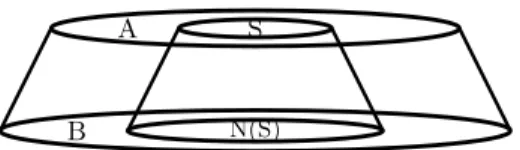
We first consider the case whereG= (A∪B, E)is bipartite. To explain the basic idea, we introduce the following concept (illustrated in Figure 1).
Definition. LetG = (A∪B, E) be a bipartite graph of ordern = |A|+|B|
without isolated notes and assume without loss of generality that|A| ≤ |B|. Let
λ≤ 1
A S
B N(S)
Fig. 1.A well-spread bipartite graph.
with parameterλif for all S⊆Awe have
|S| |N(S)| ≤ |A| |B| = λ 1−λ.
(Here, as usual,N(S)⊆B denotes the set of neighbors ofS inB.)
Examples of well-spread bipartite graphs are biregular graphs or biregular graphs minus an edge. Note that ifGis well-spread with parameterλ≤ 1
2, then Hall’s condition|N(S)| ≥ |S|for all S ⊆A is satisfied, implying that A can be com-pletely matched to B (see, for example, [22]). The following lemma is the key observation.
Lemma 1. Let G = (A∪B, E) be well-spread with parameter λ ≤ 1 2. Then
p≡λonB andp≡1−λonA yieldsαG≤ 14n.
Proof. AssumeL⊆N is an independent set. Letρ≤1such that|L∩A|=ρλn. Since Gis well-spread, we get |N(L∩A)| ≥ρ(1−λ)n, so that|L∩B| ≤(1−
ρ)(1−λ)n. Thusp(L) =|L∩A|(1−λ)+|L∩B|λ≤ρλn(1−λ)+(1−ρ)(1−λ)nλ≤
ρ14n+ (1−ρ)14n≤ 1
4n. ut
In general, whenG= (A∪B, E) is not well-spread, we seek to decompose
G into well-spread induced subgraphs Gi = (Ai∪Bi, Ei) with A = SAi and B =SB
i. Of course, this can only work ifG= (A∪B, E)is such that Acan be matched toB inG.
Proposition 1. LetG= (A∪B, E)be a bipartite graph without isolated vertices and assume thatAcan be matched intoB. ThenGdecomposes into well-spread induced subgraphs Gi = (Ai∪Bi, Ei), with A=SAi andB =SBi in such a way that for alli, j with i < j,λi ≥λj and no edges joinAi toBj.
Proof. Let S ⊆ A maximize|S|/|N(S). SetA1 :=S and B1 :=N(S). Let G0 be the subgraph ofGinduced byA\A1 andB0 :=B\B1. Then G0 satisfies the assumption of the Proposition. Indeed, if A0 cannot be matched into B0 in G0,
then there must be someS0 ⊆A0with|S0|>|N0(S0)|, whereN0(S0) =N(S0)\B
1 is the neighborhood ofS0 inG0. But then|S∪S0|=|S|+|S0|and|N(S∪S0)| ≤ |N(S)|+|N0(S)| shows that S cannot maximize |S|/|N(S)|, a contradiction. Thus, by induction, we may assume thatG0 decomposes in the desired way into well-spread subgraphs G2, . . . , Gk with parameters λ2 ≥ · · · ≥ λk. The claim then follows by observing that (i) no edges join B1 to A0; and (ii) λ1 ≥ λ2 (otherwiseS∪A2would contradict the choice ofS maximizing|S|/|N(S)|). ut
We combine the last two results.
Corollary 1. For every bipartite graph G = (A∪B, E) of order n satisfying the assumption of Proposition 1, there exists a payoff vector p ≥ 0 such that pi+pj ≥1 forij ∈E and p(L)≤ 14n for any independent setL ⊆A∪B. In addition,pcan be chosen so as to satisfyp≥ 1
2 onA.
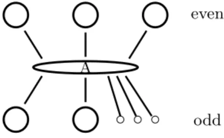
Proof. The result follows immediately from Lemma 1 and Proposition 1. Note that ifpis chosen asp≡1−λi onAi, then it holds thatp≥12 indeed. ut As we will see, the assumption of Proposition 1 is not really restrictive for our purposes. A (connected) componentC of a graph Giseven (odd) ifC has an even (odd) number of vertices. A graph G = (N, E) is factor-critical if for every vertex v ∈V(G), the graph G−v has a perfect matching. We recall the well-known Gallai–Edmonds Theorem (see [22]) for characterizing the structure of maximum matchings inG; see also Figure 2. There exists a (unique) subset
A⊆N, called aTutte set, such that (i) every even component of G−Ahas a perfect matching; (ii) every odd component ofG−A is factor-critical; and (iii) every maximum matching inGis the union of a perfect matching in each even component, a nearly perfect matching in each odd component and a matching that matchesA(completely) to the odd components.
A
even
odd
Fig. 2.Tutte setAsplittingGinto even and odd components (possibly single nodes).
We are now ready to derive our first main result.4
Theorem 1. Let G= (N, E)be a graph of ordern. ThenαG≤ 14n.
Proof. Let A⊆ N be a Tutte set. Contract each odd component in G−A to a single vertex and let B denote the resulting set of vertices. The subgraphG¯
induced byA∪Bthen satisfies the assumption of Corollary 1. Let p¯∈R|A|+|B|
be the corresponding payoff vector. We definep∈Rnby settingp
i= ¯pifor every vertexi∈Aand every vertexithat corresponds to an odd component of size1
in G−A. All other vertices getpj= 12.
It is straightforward to check thatp≥ 0 and pi+pj ≥1. Indeed, it holds that p¯ ≥ 1
2 everywhere except on B, so the only critical edges ij have i ∈ A
4
Fornis odd, the upper bound in Theorem 1 can be slightly strengthened ton2−1 4n [18].
andj a singleton odd component. But in this casepi+pj = ¯pi+ ¯pj ≥1. Thus we are left to prove that for every independent setL ⊆N, p(L)≤ 1
4n. Let B0 denote the set of singleton odd componentsi∈B,L0:= (L∩A)∪(L∩B0)and
n0:=|A|+|B|. Clearly,L0 is an independent set in the bipartite graphG¯ , and
p≡p¯onL0. We thus conclude thatp(L0)≤ 14n0.
Next let us analyzeL∩C where C⊆N\A is an even component. As C is perfectly matchable,Lcontains at most|C|/2vertices ofC. Sop(L∩C)≤ 1
4|C|. A similar argument applies to the odd components. LetCbe an odd component inG−Aof size at least3. Then certainlyLcannot contain all vertices ofC, so there exists somei∈C\L. SinceCis factor-critical,C\iis perfectly matchable, implying thatLcan contain at most half ofC\i. Thus|L∩C| ≤(|C| −1)/2and
p(L∩C)≤(|C| −1)/4.
Summarizing,n−n0=|N| −(|A|+|B|)is the sum over all|C|, whereC is an even component plus the sum over all|C| −1whereCis an odd component, andp(L\L0)is at most a 14 fraction of this, finishing the proof. ut We note that both decompositions that we use to define the payoff pcan be computed efficiently. For the Edmonds–Gallai decomposition, this is a well-known fact (see, for example, [22]). For the decomposition into well-spread sub-graphs, this follows from the observation that deciding whethermaxS |
S| |N(S)| ≤r
is equivalent tominSr|N(S)| − |S| ≥0, which amounts to minimizing the sub-modular function f(S) = r|N(S)| − |S|; see, for example, [26] for a strongly polynomial-time algorithm.
We now deal with the more general case where there are, in addition, minimal winning coalitions of size 4 or larger. First recall how the payoff p that we proposed in Corollary 1 works. For a bipartite graph G = (A∪B, E) that is split into well-spread subgraphs Gi = (Ai∪Bi, Ei) with parameterλi, we let p ≡ λi on Bi. So for λi < 14, pmay be infeasible, that is, we may encounter winning coalitions W of size 4 or larger with p(W) < 1. This problem can easily be remedied by raising pa bit on each Bi and decreasing it accordingly on Ai. Indeed, the standard (λ,1−λ) allocation rule proposed in Lemma 1 is based on the simple fact that λ(1−λ)≤ 1
4, which gives us some flexibility for modification in the case whereλis small. More precisely, defining the payoff to be
p:≡ 1 4(1−λ)>
1
4 onB and1−p < 3
4 onAfor a bipartite graph(G= (A∪B, E), well-spread with parameter λ, would work as well and thus solve the problem. Indeed, the unique independent setLthat maximizesp(L)isL=Bin this case, which givesp(L) =p(B) =|B|/(4(1−λ)) = 14n.
There is one thing that needs to be taken care of. Namely, in Proposition 1 we assumed thatG= (A∪B, E)has no isolated vertices, an assumption that can be made without loss of generality if we only have2-element winning coalitions. Now we may have isolated vertices that are part of winning coalitions of size4
or larger. But this does not cause any problems either. We simply assignp:= 1 4 to these isolated vertices to ensure that indeed all winning coalitions W have
p(W)≥1. Formally, this can also be seen as an extension of our decomposition: if G= (A∪B, E)contains isolated vertices, then they are all contained in B
vertices can be seen as a “degenerate” well-spread final subgraph(Ak∪Bk, Ek) with Ak = ∅ and parameter λk = 0. Our proposed payoff p≡ 4(1−1λk) would then indeed assignp= 14 to all isolated vertices.
It remains to observe that when we pass to general graphs, no further prob-lems arise. Indeed, all that happens is that vertices in even and odd components get payoffsp= 12 which certainly does no harm to the feasibility ofp. Thus we have proved the following result.
Corollary 2. Let (N, v)be a simple game with no minimal winning coalition of size3. Thenα(N, v)≤ 1
4n.
We end this section with the complementary case where all minimal winning coalitions have size3.
Proposition 2. Let(N, v)be a simple game with all minimal winning coalitions of size 3. Thenα(N, v)≤1
4n.
Proof. We tryp:≡ 1
3, which is certainly feasible. If this yieldsmaxp(L)≤ 1 4n, then we are done. Otherwise, there exists a losing coalitionL⊆N withp(L) =
1 3|L|>
1
4n, or equivalently,|L| > 3
4n. In this case we use an alternative payoff
˜
p given by p˜≡ 1 on N\L and p˜≡ 0 on L. Since |N \L| < 14n, this ensures
˜
p( ˜L)< 14n for any losing coalition L˜. On the other hand, p˜is feasible, since a winning coalitionW cannot be completely contained in L, that is, there exists a playeri∈W withp˜i= 1 and hencep˜(W)≥1. ut We note that Proposition 2 is a pure existence result. To computep˜it requires to solve a maximum independent set problem in 3-uniform hypergraphs, which isNP-hard. This can be seen from a reduction from the maximum independent set problem in graphs, which is well known to be NP-hard (see [15]). Given a graph G= (V, E), construct a3-uniform hypergraphG¯ as follows. Addn=|V|
new vertices labeled 1, . . . , n and extend each edge e = ij ∈ E to n edges
{i, j,1}, . . . ,{i, j, n} in G¯. It is readily seen that a maximum independent set of vertices inG¯ (that is, a set of vertices that does not contain any hyperedge) consists of thennew vertices plus a maximum independent set inG.
3
Minimal Winning Coalitions of Arbitrary Size
In this section we try to combine the ideas for the two complementary cases to derive an upper boundα≤ 2
7for the general case. The payoffspthat we consider will all satisfyp≥1
4 so that only winning coalitions of size2and3are of interest. The basic idea is to start with a bipartite graph(A∪B, E)representing the size2
winning coalitions and a payoff satisfying all these. Standard payoffs that we use satisfy p ≥ 1
4 on B and p ≥ 1
2 on A. Hence we have to worry only about 3 -element winning coalitions contained in B. We seek to satisfy these by raising the payoff of some vertices inB without spending too much in total.
More precisely, consider a bipartite graphG= (A∪B, E)representing the winning coalitions of size 2. As before, we assume that A can be completely
matched into B, so that our decomposition into well-spread subgraphs Gi =
(Ai∪Bi, Ei)applies (with possibly the last subgraphGk = (Ak∪Bk, Ek)having Ak = ∅ and Bk consisting of isolated points, as explained at the end of the previous section). Recall the payoff¯λi :≡4(1−1λ
i) onBiand1−
¯
λionAidefined for the proof of Corollary 2. We first consider the following payoff p¯:≡1−λ¯i on Ai and p¯ :≡ λ¯i on Bi for λi ≥ 14, so ¯λi ≥ 13. For subgraphs with λi < 14 (including possibly a finalλk = 0) we definep¯≡23 onAiandp¯≡ 13 onBi. Thus it holds that p¯≥ 1
3 everywhere, in particular, p¯is feasible with respect to all winning coalitions of size at least 3.
Let L¯ be a losing coalition with maximum p¯(L). We define an alternative payoffp˜as follows: Forλi≥ 41 we setp˜:≡1−λ¯i onAi, p˜:≡¯λi onB∩L¯ and
˜
p:≡ 1
2 onBi\L¯. Forλi<14 we setp˜:≡ 3
4 onAi, p˜:≡ 14 onBi∩L¯andp˜:≡12 on
Bi\L¯. Clearly, bothp¯andp˜are feasible. We claim that a suitable combination of these two yields the desired upper bound (proof omitted) yielding Theorem 2.
Lemma 2. Forp:= 3 7p¯+ 4 7p˜we getα= maxL p(L)≤ 2 7n.
Theorem 2. For every simple game(N, v),α(N, v)≤ 2 7n.
4
Complete Simple Games
Intuitively, the class of complete simple games is “closer” to weighted voting games than general simple games. The next result quantifies this expectation.
Theorem 3. A complete simple game(N, v) hasα≤√nlnn.
Proof. Let N = {1, . . . , n} be the set of players and assume without loss of generality that 1 2 · · · n. Let k ∈ N be the largest number such that
{k, . . . , n}is winning. Fori= 1, . . . , k, letsidenote the smallest size of a winning coalition in {i, . . . , n}. Definepi := 1/si for i = 1, . . . , k and pi :=pk for i = k+ 1, . . . , n. Thus, obviously,p1≥ · · · ≥pk =· · ·=pn.
Consider a winning coalitionW ⊆N and letibe the first player inW (with respect to). If|W| ≤√n, then si≤ |W| ≤
√
nand hencep(W)≥pi= s1i ≥
1
√
n. On the other hand, if|W|>
√
n, thenp(W)>√npk ≥
√
n1n = √1 n. For a losing coalition L ⊆ N, we conclude that |L∩ {1, . . . , i}| ≤ si−1 (otherwise L would dominate the winning coalition of sizesi in {i, . . . , n}). So p(L)is bounded bymaxPk
i=1xis1i subject to P i
j=1xj ≤si−1, i= 1, . . . , k. The optimal solution of this maximization problem is x1 = s1−1, xi = si− si−1for2≤i≤k. Hencep(L)≤(s1−1)s11+ (s2−s1)s12+· · ·+ (sk−sk−1)s1k ≤ 1 2+· · ·+ 1 sk ≤lnn. Summarizing, we obtain p(L)/p(W)≤ √ nlnn. ut
In [12] it is conjectured thatα=O(√n)holds for complete simple games. In the same paper a lower bound of order√nis given, as well as specific subclasses of complete simple games for whichα=O(√n)can be proven.
5
Algorithmic Aspects
A fundamental question concerns the complexity of our original problem (1). For general simple games this depends on how the game in question is given, and we refer to Section 1 for a discussion. Here we concentrate on the graphic” case.
Proposition 3. ComputingαGfor bipartite graphsGcan be done in polynomial time.
Proof. LetP ⊆RnBe the set of feasible payoffs (satisfyingp≥0andpi+pj ≥1 forij ∈E). Forα∈R, letPα:={p∈P|p(L)≤αfor all independent L⊆N}. Thus αG = min{α | Pα 6= ∅}. The separation problem for Pα (for any given α) is efficiently solvable. Given p ∈ Rn, we can check feasibility and whether max{p(L) | L ⊆ N independent} ≤ α by solving a corresponding maximum weight independent set problem in the bipartite graph G. Thus we can, for any given α ∈ R, apply the ellipsoid method to either compute some p ∈ Pα or conclude thatPα=∅. Binary search then exhibits the minimum value for which Pαis non-empty; binary search works indeed in polynomial time as the optimal αhas size polynomially bounded inn, which follows from observing that
α= min{a|pi+pj≥1 ∀ij∈E, p(L)−a≤0 ∀L⊆N independent, p≥0} (3) can be computed by solving a linear system ofnconstraints defining an optimal basic solution of the above linear program. ut
The proof of Proposition 3 also applies to other classes of graphs, such as claw-free graphs (see [6]) in which finding a weighted maximum independent set is polynomial-time solvable. In general, the problem isNP-hard.
Proposition 4. ComputingαG for arbitrary graphsGisNP-hard.
Proof. LetG0 = (N0, E0)andG00 = (N00, E00) be two disjoint copies of a graph
G= (N, E)with independence number k. For eachi0∈N0 andj00∈N00add an edgei0j00if and only ifi=jorij∈Eand call the resulting graphG∗= (N∗, E∗). We claim thatαG∗=k/2(thus computingαG∗ is as difficult as computing k).
First note that the independent sets in G∗ are exactly the sets L∗ ⊆ N∗
that arise from an independent set L ⊆ N in G by splitting L into two com-plementary sets L1 and L2 and defining L∗ := L01∪L002. Hence, p≡
1 2 onN
∗
yields maxp(L∗) = k/2 where the maximum is taken over all independent sets
L∗⊆N∗ inG∗. This shows thatαG∗≤k/2.
Conversely, letp∗be any feasible payoff inG∗, that is,p∗≥0andp∗i+p∗j ≥1
for all ij ∈ E∗. Let L⊆N be a maximum independent set of sizek in G and
construct L∗ by including for each i ∈ L either i0 or i00 in L∗, whichever has p-value at least 1
2. Then, by construction, L
∗ is an independent set in G∗ with p∗(L∗)≥k/2, showing that αG∗≥k/2. ut
Summarizing, for graphic simple games, computing αG is as least as hard as computing the size of a maximum independent in G. For our last result we assume thatais a fixed integer, that is,ais not part of the input.
Proposition 5. For every fixed a > 0, it is possible to decide if αG ≤ a in polynomial time for an arbitrary graph G= (N, E).
Proof. Letk= 2da+efor some >0. By brute-force, we can check inO(n2k) time ifN contains2kvertices{u1, . . . , uk} ∪ {v1, . . . , vk} that inducek disjoint copies of P2, that is, paths Pi = uivi of length 2 for i = 1, . . . , k with no edges joining any two of these paths. If so, then the conditionp(ui) +p(vi)≥1 implies that one of ui, vi, say ui, must receive a payoff p(ui) ≥ 12, and hence U ={u1, . . . , uk}hasp(U)≥k/2> a. AsU is an independent set,α(G)> a.
Now assume that Gdoes not contain k disjoint copies of P2 as an induced subgraph, that is,Gis kP2-free. For everys≥1, the number of maximal inde-pendent sets in a sP2-free graphs isnO(s) due to a result of Balas and Yu [2]. Tsukiyama, Ide, Ariyoshi, and Shirakawa [30] show how to enumerate all maxi-mal independent sets of a graphGonnvertices andmedges using timeO(nm)
per independent set. Hence we can find all maximal independent sets of Gand thus solve, in polynomial time, the linear program (3). Then it remains to check if the solution found satisfiesα≤a. ut
6
Conclusions
After our paper appeared, Kanstantsin Pashkovich [1] found a proof of Conjec-ture 1. Hence it remains to tighten the upper bound for complete simple games to O(√n). In order to classify simple games, many more subclasses of simple games have been identified in the literature. Besides the two open problems, no optimal bounds for αare known for other subclasses of simple games, such as strong, proper, or constant-sum games, that is, where v(S) +v(N\S) ≥ 1,
v(S) +v(N\S)≤1, orv(S) +v(N\S) = 1for allS ⊆N, respectively.
Acknowledgments. The second and fourth author thank Péter Biró and Hajo Broersma for fruitful discussions on the topic of the paper.
References
1. K. Pashkovich. On critical threshold value for simple games. arXiv:1806.03170v2, 11 June 2018.
2. E. Balas and C. S. Yu. On graphs with polynomially solvable maximum-weight clique problem. Networks, 19(2):247–253, 1989.
3. J. M. Bilbao, J. R. F. García, N. Jiménez, and J. J. López. Voting power in the European Union enlargement.Eur. J. Operational Research, 143(1):181–196, 2002. 4. P. Biro, W. Kern, and D. Paulusma. Computing solutions for matching games.
International Journal of Game Theory, 41:75–90, 2012.
5. A. Bock, K. Chandrasekaran, J. Könemann, B. Peis, and L. Sanitá. Finding small stabilizers for unstable graphs. Mathematical Programming, 154:173–196, 2015. 6. A. Brandstaett and R. Mosca. Maximum weight independent set in lclaw-free
7. G. Chalkiadakis, E. Elkind, and M. Wooldridge. Computational Aspects of Coop-erative Game Theory. Morgan and Claypool Publishers, 2011.
8. V. G. Deineko and G. J. Woeginger. On the dimension of simple monotonic games.
European Journal of Operational Research, 170(1):315–318, 2006.
9. E. Elkind, G. Chalkiadakis, and N. R. Jennings. Coalition structures in weighted voting games. volume 178, pages 393–397, 2008.
10. E. Elkind, L. A. Goldberg, P. W. Goldberg, and M. Wooldridge. On the computa-tional complexity of weighted voting games. Annals of Mathematics and Artificial Intelligence, 56(2):109–131, 2009.
11. U. Faigle, W. Kern, S. Fekete, and W. Hochstaettler. The nucleon of cooperative games and an algorithm for matching games.Mathematical Programming, 83:195– 211, 1998.
12. J. Freixas and S. Kurz. On α-roughly weighted games. International Journal of Game Theory, 43(3):659–692, 2014.
13. J. Freixas, X. Molinero, M. Olsen, and M. Serna. On the complexity of problems on simple games. RAIRO-Operations Research, 45(4):295–314, 2011.
14. J. Freixas and M. A. Puente. Dimension of complete simple games with minimum.
European Journal of Operational Research, 188(2):555–568, 2008.
15. M. R. Garey and D. S. Johnson. Computers and Intractability: A Guide to the Theory of NP-Completeness. W. H. Freeman & Co., New York, NY, USA, 1979. 16. T. Gvozdeva, L. A. Hemaspaandra, and A. Slinko. Three hierarchies of simple
games parameterized by “resource” parameters. International Journal of Game Theory, 42(1):1–17, 2013.
17. T. Hegedüs and N. Megiddo. On the geometric separability of Boolean functions.
Discrete Applied Mathematics, 66(3):205–218, 1996.
18. F. Hof. Weight distribution in matching games. MSc Thesis, University of Twente, 2016.
19. W. Kern and D. Paulusma. Matching games: The least core and the nucleolus.
Mathematics of Operations Research, 28:294–308, 2003.
20. J. Koenemann, K. Pashkovich, and J. Toth. Computing the nucleolus of weighted cooperative matching games in polynomial time. arXiv:1803.03249v2, 9 March 2018.
21. S. Kurz, X. Molinero, and M. Olsen. On the construction of high dimensional simple games. In Proc. ECAI 2016, pages 880–885, New York, 2016.
22. L. Lovász and M. D. Plummer. Matching theory, volume 367. American Mathe-matical Society, 2009.
23. U. N. Peled and B. Simeone. Polynomial-time algorithms for regular set-covering and threshold synthesis. Discrete Applied Mathematics, 12(1):57–69, 1985. 24. H. Peters. Game Theory. Springer, 2008.
25. J. R. Isbell. A class of majority games.Quarterly J. Mathematics, 7:183–187, 1956. 26. A. Schrijver. A combinatorial algorithm minimizing submodular functions in
strongly polynomial time. J. Comb. Theory, Ser. B, 80(2):346–355, 2000. 27. T. Solymosi and T. E. Raghavan. An algorithm for finding the nucleolus of
assign-ment games. International Journal of Game Theory, 23:119–143, 1994.
28. A. D. Taylor and W. S. Zwicker. Weighted voting, multicameral representation, and power. Games and Economic Behavior, 5:170–181, 1993.
29. A. D. Taylor and W. S. Zwicker. Simple games: Desirability relations, trading, pseudoweightings. Princeton University Press, 1999.
30. S. Tsukiyama, M. Ide, H. Ariyoshi, and I. Shirakawa. A new algorithm for gener-ating all the maximal independent sets. SIAM J. Computing, 6(3):505–517, 1977.