Decarbonising Future Power Systems by Demand Side Management in Smart Grid

(1)

Durham E-Theses

Decarbonising Future Power Systems by Demand Side

Management in Smart Grid

LI, DAN

How to cite:

LI, DAN (2019) Decarbonising Future Power Systems by Demand Side Management in Smart Grid, Durham theses, Durham University. Available at Durham E-Theses Online:

http://etheses.dur.ac.uk/12988/

Use policy

The full-text may be used and/or reproduced, and given to third parties in any format or medium, without prior permission or charge, for personal research or study, educational, or not-for-prot purposes provided that:

• a full bibliographic reference is made to the original source

• alinkis made to the metadata record in Durham E-Theses

• the full-text is not changed in any way

The full-text must not be sold in any format or medium without the formal permission of the copyright holders. Please consult thefull Durham E-Theses policyfor further details.

(2)

Academic Support Oce, Durham University, University Oce, Old Elvet, Durham DH1 3HP e-mail: [email protected] Tel: +44 0191 334 6107

http://etheses.dur.ac.uk

(3)

Decarbonising Future Power Systems

by Demand Side Management

in Smart Grid

Dan Li

A Thesis presented for the degree of

Doctor of Philosophy

Department of Engineering

University of Durham

United Kingdom

August 2018

(4)

Decarbonising Future Power Systems by Demand

Side Management in Smart Grid

Dan Li

Abstract

Carbon emission reduction is an urgent global task. Renewable energy sources integration can promote the transformation of cleaner and greener power system. But the time-varying nature of these sources causes indeterminacy problems. Smart grid is a powerful tool that can deal with these problems in electricity aspect. One of the key smart grid technologies is demand side management. How to use demand side management to regulate and decarbonise the power system is the main point of this thesis.

In order to integrate renewable energy sources, a day-ahead electricity market scheme is proposed, involving the utility, the demand response aggregator and cus-tomers. This model leads to a multiobjective optimization problem, which is solved by an artificial immune algorithm. The simulation results confirm the feasibility and robustness of the proposed model. All participants can benefit from it, and the system power peak to average ratio can be reduced.

In order to realize the carbon emission reduction, a system model for annual fuel sources scheduling and operational policy making of electricity generation is established, considering the economic, environmental and social aspects. A mini-mum Manhattan distance approach is proposed to select the final solution. The impacts of carbon tax and renewable obligation on carbon emission, generation cost and electricity bill are examined. These can reveal the proper strategy for deciding renewable energy source and carbon emission related policies.

After that, a carbon emission flow model is introduced to facilitate the analysis and assessment of demand side management’s impacts on carbon emission reduction. The time sensitivity of carbon emission in both generation side and customer side are obtained. The daily case and seasonal case are presented. The simulation results show that the load curtailment and load shift approaches can effectively reduce the carbon emission.

(5)

Declaration

The work in this thesis is based on research carried out at the Department of En-gineering, Durham University, United Kingdom. No part of this thesis has been submitted elsewhere for any other degree or qualification and it is all my own work unless referenced to the contrary in the text.

Copyright c 2018 by Dan Li.

“The copyright of this thesis rests with the author. No quotations from it should be published without the author’s prior written consent and information derived from it should be acknowledged”.

(6)

Acknowledgements

First, I would like to thank my supervisors, Dr. Hongjian Sun and Prof. Simon Hogg at Durham University, and Dr. Wei-Yu Chiu at National Tsing Hua University, for the excellent guidance they provided over the past four years. Their endless patience and enthusiasm keep me always stay positive during the whole of my PhD time. I have learned a great deal from the enjoyable discussions and interacting with them. Thanks to all my colleagues: Weiqi Hua, Qitao Liu, Minglei You, Jiangjiao Xu, Xiaolin Mou, Hao Xiao, Tianying Xiao and Meng Xu, for their assistance and discussions about my work. Because of their help and encouragement, I spent a good time during my PhD.

Also thanks to all of my friends in the U.K., especially to Lei Fan, Yanjun Tan, Difu Shi, Yi Sun, Jing Zhang, Yuexian Hong, Ang Li, Manjun Liu, Min Yao, Xudong Chen, and Konstantinos Krestenitis. They made my PhD life so colourful. I will never forget the laughter and tears with all of them. Wish our friendships built in this country would keep on forever.

Finally, I am deeply thankful to my dearest Mum and Dad for the support not only during the PhD, but during all my life. Whenever I have been depressed, their gentle concerns can always encourage me to carry on.

(7)

Publication List

•

Book Chapter

– Dan Li, Wei-Yu Chiu and Hongjian Sun,“Demand Side Management in

Microgrid Control Systems.”, In Microgrid: Advanced Control Methods

and Renewable Energy System Integration. Mahmoud, Magdi S. Elsevier.

•

Journal Paper

– Dan Li, Hongjian Sun, Wei-Yu Chiu and Poor Vincent, “

Multiobjec-tive Optimization for Demand Side Management in Smart Grid.”, IEEE

Transactions on Industrial Informatics 14(4): 1482-1490.

– Dan Li, Weiqi Hua, Hongjian Sun and Wei-Yu Chiu, “ Carbon

Emis-sion Reduction in Electricity Generation: Minimum Manhattan Distance

approach”, IET Smart Gird, In process.

– Weiqi Hua, Dan Li, Hongjian Sun, Peter Matthew, and Fanlin Meng,

“ Stochastic Environmental and Economic Dispatch of Power Systems

with Virtual Power Plant in Energy and Reserve Markets”, International

Journal of Smart Grid and Clean Energy, accepted in May 2018.

– Weiqi Hua, Dan Li, Hongjian Sun and Peter Matthew, “Stackelberg

Game-theoretic Model for Low Carbon Energy Market Scheduling”, IET

Smart Grid, submitted in July 2018.

•

Conference Paper

– Dan Li, Hongjian Sun and Wei-Yu Chiu, “ A Layered Approach for

Enabling Demand Side Management in Smart Grid.”, 2016 International

(8)

vi Conference on Control, Automation and Information Sciences (ICCAIS). Ansan, Korea, IEEE, 54-59.

– Dan Li, Weiqi Hua, Hongjian Sun and Wei-Yu Chiu, “ Multiobjective

Optimization for Carbon Market Scheduling based on Behavior

Learn-ing”, 2017 International Conference on Applied Energy. Cardiff, Energy

Procedia 142 (2017): 2089-2094.

– Dan Li, Hongjian Sun and Wei-Yu Chiu,“ Achieving Low Carbon

Emis-sion using Smart Grid Technologies”, 2017 IEEE 85th Vehicular

Tech-nology Conference (VTC2017). Sydney, IEEE, Piscataway, 1-5.

– Weiqi Hua, Dan Li, Hongjian Sun and Peter Matthew, “Unit

Commit-ment in Achieving Low Carbon Smart Grid EnvironCommit-ment with Virtual

Power Plant”, 2017 IEEE International Smart Cities Conference (ISC2).

(9)

List of Figures

1.1 Electricity generation mix by major fuel sources in the U.K. from

2000 to 2017 [6]. . . 3

1.2 Carbon emission from electricity generation by major fuel sources in the U.K. from 2000 to 2017 [8]. . . 3

2.1 Demonstration of peak clipping. . . 13

2.2 Demonstration of valley filling. . . 13

2.3 Demonstration of load shifting. . . 14

2.4 Demonstration of strategic conservation. . . 15

2.5 Demonstration of strategic load growth. . . 15

2.6 The electricity market share by sectors in the U.K. in 2017 [29]. . . . 16

2.7 Demonstration of ToU pricing. . . 22

2.8 Demonstration of critical peak pricing. . . 22

2.9 Demonstration of real time pricing. . . 23

2.10 Functionality of the DR aggregator in a power grid [54]. . . 24

2.11 Structure of fuel source scheduling problems [76,77]. . . 29

3.1 System operation model. . . 37

3.2 Example of a Pareto front. . . 46

3.3 Example of a Pareto optimality. . . 46

3.4 Flowchart of the AIA algorithm. . . 48

3.5 The wind turbine output performance [130]. . . 52

3.6 The wind turbine output for the selected day. . . 52

3.7 The APF for the proposed MOP. . . 54

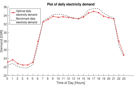
3.8 The optimized usage pattern for the day-ahead market. . . 54 x

(13)

List of Figures xi

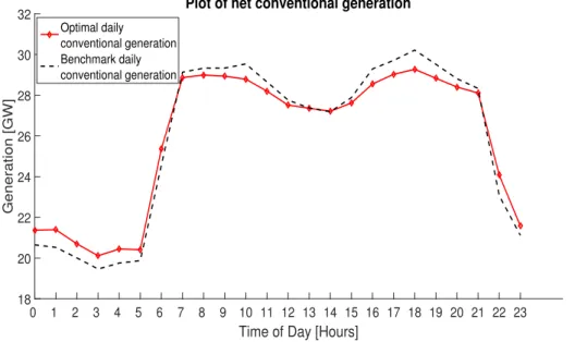
3.9 The net conventional generation for the day-ahead market. . . 55

3.10 The comparison of optimization results and benchmark in Case 1. . . 57

3.11 The comparison of optimization results and benchmark in Case 2. . . 58

3.12 The comparison of original optimal and disturbed optimal results in Case 3 and Case 4. . . 59

3.13 The system performance with the change of compensation coefficient α 62 3.14 The system performance with the change of inelasticity coefficient ε . 64 4.1 The system operation model. . . 68

4.2 An example of the knee solution. . . 74

4.3 Demonstration of MMD approach to MCDM. . . 76

4.4 Demonstration of WS approach to MCDM. . . 77

4.5 Demonstration of D & C approach to MCDM. . . 79

4.6 The MMD approach for a 3-D MOP. . . 81

4.7 The WS approach for a 3-D MOP. . . 81

4.8 The D & C approach in two random comparing orders for the MOP. . 82

4.9 The APF for the proposed MOP. . . 84

4.10 Comparison of the fuel usage plan for electricity generation in short-term period. . . 86

4.11 Comparison of the electricity generation by major fuel sources in short-term period. . . 87

4.12 Comparison of the fuel usage plan for electricity generation in the short-term period and long-term period. . . 89

4.13 Comparison of the electricity generation by major fuel sources in the short-term period and long-term period. . . 90

4.14 The system performance with the change of compensation coefficient α. . . 92

4.15 The system performance with the change of additional operating cost coefficient γ. . . 93

4.16 The system performance with the change of carbon tax rate m. . . . 95

(14)

List of Figures xii

5.1 Demonstration of the CEF model by an IEEE 5-bus system. . . 102

5.2 Demonstration of proportional sharing principle. . . 104

5.3 Relationship between branch power flow and node power flow. . . 105

5.4 The CEF model of an IEEE 30-bus system. . . 110

5.5 Daily ICEF for bus 3 and bus 20. . . 112

5.6 Daily ECEF performance with respect to load curtailments on 5th May. 2017. . . 114

5.7 Daily ECEF performance with respect to load shift and curtailment on 5th May. 2017. . . 115

5.8 Daily ECEF performance on 14th Jan. 2017. . . 117

5.9 Daily ECEF performance on 14th Jun. 2017. . . 117

(15)

List of Tables

2.1 Summary of the smart grid projects . . . 8

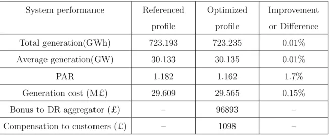
3.1 Comparison of the reference and the optimal system performance . . 56

3.2 Results of the system performance in Case 1 and Case 2 . . . 58

3.3 Results of the original optimal and disturbed optimal system perfor-mance in Case 3 and Case 4 . . . 59

3.4 The system performance with the change of bonus coefficient µ . . . 61

4.1 Coefficients for the proposed model . . . 80

4.2 Computation time for WS, D & C and MMD approaches . . . 83

4.3 System performance for different solutions . . . 84

5.1 ECEF calculation for generators . . . 109

5.2 ICEF results for buses . . . 109

5.3 BCEF & BCEL results for branches . . . 109

5.4 ECEF calculation for generators . . . 112

5.5 CEF performance on 5th May. 2017 . . . 116

(16)

List of Symbols and Abbreviations

:= Assignment operator.

α, β Compensation coefficient.

γ Additional operating cost coefficient.

µ Bonus coefficient.

ω Weight coefficient in the WS approach.

ψ Wind turbine blade pitch angle.

ρ Air density.

σ Wind turbine performance coefficient.

τ Wind turbine blade tip speed ratio.

θ Mutate coefficient.

ε Dissatisfactory coefficient.

ς Wind turbine blade swept area.

IB BCEF intensity.

IG ECEF intensity.

II ICEF intensity.

IL BCEL intensity.

P1

B Branch active power inflow matrix.

(17)

List of Symbols and Abbreviations xv

PB Branch active power outflow matrix.

PG Active power ejection matrix.

PI Active power injection matrix.

PN Node power flow matrix.

RB BCEF rate.

RG ECEF rate.

RI ICEF rate.

RL BCEL rate.

diag Diagonal matrix operator.

A Antibodies collection.

bi Generation cost coefficient for sourcei.

c0 Conventional generation cost without the DSM.

c1 _{Conventional generation cost with the DSM.}

cres _{RESs generation cost.}

d0 Total electricity demand before the DSM.

d1 _{Total electricity demand after the DSM.}

ei Carbon emission coefficient for source i.

F(·) Multiobjective problem.

fa(·) Objective function for the aggregator.

fc(·) Objective function for customers.

fp(·) Objective function for the policy maker.

(18)

List of Symbols and Abbreviations xvi

fbas(·) Basic cost function of fuel sources for utilities. fbon(·) Bonus function for the aggregator.

fcom(·) Compensation function for customers.

fct(·) Carbon tax function for utilities. fdis(·) Dissatisfactory function for customers. fe(·) CEF function.

ff it(·) Fitness function.

fgene(·) Total generation cost function for utilities. fope(·) Additional operating cost function for utilities.

fro(·) Extra generation cost function for utilities due to the Renewable Obligation.

g0

i Generation from source i before generation adjustment.

g_i1 Generation from source i after generation adjustment.

gc

t Power obtained from conventional generators at time slot t.

gres

t Power obtained from RESs at time slot t.

gt Expected power generation at time slot t.

gdown Power ramp down limit.

gi,r Generation from RESs.

gup Power ramp up limit.

G Expected power generation from conventional generators.

h Price of the renewable energy certificate.

J Number of objectives.

l0

(19)

List of Symbols and Abbreviations xvii

l1_t Demand at time slot t with the DSM.

L Total consumption of electricity in one day.

M Number of vectors in APS and APF.

m Carbon tax rate.

nc Iteration number.

Np Population size of antibodies.

p∗ Selected Pareto optimal solution.

p The vector of decision variables.

q The price of per unit electricity.

R Minimum requirement for penetration of RESs.

r Clone rate.

s0_i Fuel usage of source i before generation adjustment.

s1

i Fuel usage of source i after generation adjustment.

si,r Fuel usage of RESs.

S Spinning reserve requirement.

ui Generation coefficient for sourcei .

v Wind speed.

w Wind turbine output power.

AIA Artificial immune algorithm

APF Approximate Pareto front

APS Approximate Pareto set

(20)

List of Symbols and Abbreviations xviii BCEL Branch carbon emission loss

CEF Carbon emission flow CPF Carbon price floor D & C Divide & Conquer

DERs Distributed energy resources

DG Distributed generation

DR Demand response

DSM Demand side management DSO Distribution system operator ECEF Ejected carbon emission flow ICEF Injected carbon emission flow MCDM Multiple criteria decision making MEF Marginal emission factor

MMD Minimum Manhattan distance MOP Multiobjective optimization problem Mtoe Million tons of oil equivalent

NIP Net improvement percentage

Ofgem Office of Gas and Electricity Markets PAR Peak to average ratio

QoE Quality of experience

RESs Renewable energy sources

ToU Time-of-use

(21)

Chapter 1 Introduction

1.1 Background

Climate change has posed a threat to the sustainable development, which brings the importance of carbon emission reduction. To reduce carbon emission, the U.K. government has made significant efforts since 1997, started from the Kyoto Protocol. The U.K. committed to reducing the carbon emission by all kinds of ways, such as improving the energy efficiency, utilizing renewable energy sources (RESs), enhanc-ing the fuel standard, investenhanc-ing low-carbon technologies, and reducenhanc-ing the energy demand [1]. The U.K. was also the first country that sets a legally-binding limit on carbon emission amount. In 2008, the Climate Change Act was passed in the U.K., and the framework to develop an economically credible carbon emission reduction path was set up. It aimed to achieve at least 30% carbon emission reductions by 2020, and 80% by 2050 compared with the level of 1990 [2]. In December 2011, the U.K. government published the Carbon Plan. This plan set out how the country will transit to the decarbonization while ensuring energy security, and minimizing consumers’ cost [3].

Overall, the electricity supply plays a significant role in achieving these targets [4]. It accounts for approximately one-third of the total emission in the U.K. for the past 15 years. The average carbon emission for electricity generation was 0.7 tonne/MWh in 1990, and decreased to 0.5 tonne/MWh in 2008. The anticipated

aim is just 0.05 tonne/MWh by 2030 [5]. The monitor of fuel source usage in

(22)

1.1. Background 2 electricity supply is necessary during this transition process. Firstly, coal was the dominant source for almost half a century since 1950, contributed to 97% of the generation at 1950. Oil was generally used in the late 1950’s, and came to a peak in the early 1970’s, then impacted by the oil crisis at 1973. This gave an opportunity for the development of nuclear power. The electricity provided by it raised from 9% in 1970 to 28% in 1998. The natural gas was introduced in the 1990’s, and had a rapid increase. It exceeded the use of coal in 1990, which accounted for 39% of the generation, while coal accounted for 28%. Recently, the use of RESs scaled up. Especially, wind and solar had a significant progress, provided 15.5% of the generation in 2017 [6]. The promotion of RESs impeded the use of fossil fuel. Coal, oil, and gas experienced gradually declines. The low carbon generation in generation mix is planned to reach 61% in 2020, compared to 47% in 2015 [7]. The detailed electricity generation mix by major fuel sources from 2000 to 2017 is shown in Fig. 1.1. The changes of generation mix and evolutions of technologies result in a carbon emission reduction. The emission from power generation was reduced by 57%, from 242.1 Mtons in 1990 to 110.9 Mtons in 2016. The emission mainly came from the combustion of coal and gas. It is projected to reduce another 52% of emission till 2020, based on the level of 2015 [8]. The detailed carbon emission from electricity generation by major fuel sources from 2000 to 2017 is shown in Fig. 1.2. In the U.K., the Department for Business, Energy & Industrial Strategy (BEIS) and Office of Gas and Electricity Markets (Ofgem) are primary regulators that are responsible for the carbon emission reduction.

As mentioned before, the utilization of RESs can help with the carbon emission issue [9]. More energy is expected to be supplied by RESs in the grid, such as wind, photovoltaic, and tidal energy. However, these RESs cause intermittent problems due to their inherent characteristics. The power provided by RESs varies with the external environment conditions, e.g., season, weather and time period. The man-agement of RESs requires sophisticated planning and operation scheduling. Smart grid provides the ability for promoting the penetration of RESs. It is an intelligent power network that is composed of advanced generation, communication, control and computation technologies. It can improve the reliability, availability, and

(23)

effi-1.1. Background 3

Figure 1.1: Electricity generation mix by major fuel sources in the U.K. from 2000 to 2017 [6].

Figure 1.2: Carbon emission from electricity generation by major fuel sources in the U.K. from 2000 to 2017 [8].

(24)

1.2. Research Motivations 4 ciency of the current system [10]. Demand side management (DSM) is one of the important technologies in smart grid. It can promote the interaction and respon-siveness of customers, thus offer a wide range of potential benefits to the system and enhance the energy efficiency [11].

1.2 Research Motivations

Based on the background above, the motivations of this thesis can be summarized as follows:

• RESs are important for the electricity generation, but the inherent intermittent

characteristic is the major impediment for their developments. It is a challenge to integrate RESs into the grid.

• The DSM is considered as one of the key smart grid technologies. It is a

chal-lenge to design a feasible scheme that can efficiently regulate energy generation and consumption.

• The fuel sources planning of electricity generation for the future plays a vital

role for the sustainable development. It is a challenge to schedule the fuel sources that to meet both the environmental, economic and social require-ments.

1.3 Research Objectives

In this thesis, a daily-based demand planning scheme is firstly proposed, which involving the utility, the demand response (DR) aggregator, and customers. Then, a system model for annual fuel sources scheduling and operational policy making of electricity generation is developed, which considering the economic, environmental, and social aspects. After that, a carbon emission flow model is introduced to assess the carbon emission caused by power generation. Specifically, the focus is placed on the following four research objectives in this thesis.

(25)

1.4. Research Contributions 5

• The fuel sources scheduling and operational policy making of electricity

gen-eration

• The effectivenesses of DSM approaches on the carbon emission reduction

• Multiobjective optimization problem (MOP)

1.4 Research Contributions

The main contributions of this thesis are summarised as follows:

• An advanced electricity market scheme is proposed. For the utility, the

inher-ent intermittinher-ent problems of RESs can be addressed. For the DR aggregator, it is modelled as an independent participant. The role and the revenue of it are analysed. For customers, the social welfare is considered. All participants can benefit from the proposed design: the utility can reduce the generation cost and the power peak to average ratio (PAR); the DR aggregator can make profits by providing DR service; customers can save money on their bill. And even if there are perturbations to the system, the proposed approach can still work out an optimal solution.

• A novel system model for fuel sources scheduling and operational policy

mak-ing of electricity generation is developed. Besides economic and environmental aspects of the electricity generation, the participation of consumers is intro-duced in the model. The minimum Manhattan distance (MMD) approach is proposed to select the final optimal solution. The generation plans for both short-term period and long-term period are presented. The system sensitivity to carbon tax and Renewable Obligation are analysed. These can give a hint for formulating carbon emission and RESs related mechanisms and policies.

• A carbon emission flow model is introduced to evaluate the carbon emission

re-duction caused by DSM. The time sensitivity of carbon emission in generation side and consumption side are obtained by applying the U.K. actual daily data of electricity generation and demand. The effectivenesses of load curtailment

(26)

1.5. Thesis Outline 6 and load shift approaches for carbon emission reduction are quantified. These can indicate how to suggest different DSM programs to different consumers in the case of carbon emission reduction.

1.5 Thesis Outline

The remainder of this thesis is organized as follows: Chapter 2

In this chapter, a review of smart grid technologies is presented. A brief his-tory and basic concepts of DSM are introduced. A detailed classification of DR is discussed. The state-of-the-art models and methodologies are explained.

Chapter 3

In this chapter, a hierarchical day-ahead DSM model is proposed. The model involves three participants: the utility, the DR aggregator, and customers. This model leads to a MOP, which is solved by an artificial immune algorithm (AIA). The U.K. case study and system sensitivity analysis are presented.

Chapter 4

In this chapter, a system model for fuel usage scheduling and operational pol-icy making of electricity generation, while considering carbon emission reduction is established. A MMD approach is proposed to process the multiple criteria decision making (MCDM). The proposed approach is compared with the weighted sum (WS) approach and the divide & conquer (D & C) approach. The case studies of short-term period and long-short-term period are given. The system sensitivity is analysed.

Chapter 5

In this chapter, a carbon emission flow model is introduced. The scope of the presented model is extended by involving DSM interventions. The time sensitivity of carbon emission is obtained. The effectivenesses of load curtailment and load shift approaches on the carbon emission reduction are examined.

Chapter 6

In this chapter, the thesis is summarised and potential research directions for the future are identified.

(27)

Chapter 2 Literature Review

2.1 Introduction

Smart grid technology is a powerful tool that facilitates the process of transforming conventional grids into green systems. It can offer a two-way flow of information and a two-way flow of electricity. DSM is a vital part of it. In this chapter, DSM is investigated from various perspectives. First, a general introduction of smart grid is presented. Second, a brief history and basic concepts of DSM are introduced. Next, a detailed classification of DR is discussed. Then, state-of-the-art models and methodologies are explained.

2.2 Smart Grid

Smart grid is defined by the European Technology Platform as [12]

“an electricity network that can intelligently integrate the actions of all users connected to it generators, consumers and those that do both -in order to efficiently deliver susta-inable, economic and secure electricity supplies”.

From 1998 to 2002, the EU’s Fifth Framework Program funded the “renewable energy and distributed generation in the European power grid integration” project. Since then, smart grid has been gained great attention at the first time [13]. During

(28)

2.2. Smart Grid 8

Table 2.1: Summary of the smart grid projects

Number Budgets Organizations Implementation sites

Total: 950 projects Total: Total: 2900 Total: 800 sites

in 50 countries e 4.97 billion organizations in 36 countries

Average project Average: Average: 6 partners Average: 2.2 sites

duration: 30months e 5.75 million per project per project

Involved in more Largest Involved in more Most sites:

than one country: investments: than one projects: DE (140)

324 projects DE,UK, FR 700 organizations ES (95)

the past decades, there have been remarkable achievements in many countries. From 2002 to 2017, a total of 950 smart grid projects have been launched, amounting to

e4.97 billion investments in 50 countries. These projects always involve more than

one country (324 projects are multinational with an average of 14 countries per

project). Among all, 642 projects have been completed with the budget of e2.82

billion, 308 projects are still ongoing with the budget of e 2.15 billion. Largest

in-vestments are from Germany, the U.K. and France. The U.K. government currently has 197 projects, in which 73 projects are national. The private investment takes up a large portion in the U.K., accounting for 83% of the total national investment [14]. The detailed information can be found in Table 2.1.

Smart grid is based on the integrated high-speed bidirectional communication network, on the basis of advanced sensor and measurement technologies, advanced equipment technologies, advanced control methods, and advanced decision support systems [12]. It is made up of several parts, divided into: smart power generation system, smart substation, smart power distribution network, smart interactive ter-minal, smart scheduling, smart building electricity, smart city power grid, smart meter, smart appliance, and the new type of energy storage system [15]. Compared to the conventional power grid, smart grid has following six advantages [16, 17]:

• Based on the strong power grid system and technical support system, it can

(29)

2.3. Demand Side Management 9 grid is reinforced and ascended.

• It can obtain a panoramic view of the information, timely discover/foresee the

possibility of failure. When a fault occurs, the grid can quickly isolate the fault, realize self-recovery to avoid the occurrence of blackouts.

• The control of the grid is more flexible, and can adapt to a large number of

distributed power supplies, micro power grids, and electric vehicles.

• Through the modern management technologies, it can greatly improve the

efficiency of power equipment, and reduce the loss of transmission, making the operation of the grid is more economical and efficient.

• The highly integrated real-time and non-real-time information sharing and

uti-lization can show a comprehensive and complete grid operation state, there-fore providing decision supports, control schemes and corresponding response plans.

• By means of the two-way interactive service mode, the electric power enterprise

can obtain the user’s electricity information in detail, to provide more value-added service; users can acknowledge the real-time status of the power supply ability, power quality, price and power outage information, thus can reasonably arrange the use of electric equipment.

2.3 Demand Side Management

One of the key smart grid technologies is DSM. Electricity demand always fluc-tuates dramatically during some short time frames. Generally, to meet the de-mand, a power system adjusts the supply by increasing/decreasing the generation or adding/curtailing additional resources (e.g., RESs and energy storages) [10]. The standby generators can incur additional costs on the budget and yield system insta-bility, and there may still exist a power shortage during the peak period [18]. For these reasons, the idea of DSM has emerged.

(30)

2.3. Demand Side Management 10

2.3.1 Definition

The term “demand side management,” also known as “energy demand manage-ment,” stands for a variety of activities that are related to the energy consumption. It includes not only the control and modification of the energy usage, e.g., energy conservation, energy efficiency and energy storage, but also the behaviours that are involved in these processes, e.g., device installations, policies and regulation formu-lation, promotion, and education [10].

2.3.2 History

DSM was originated from the energy crises [19]. The first energy crisis (also called the “first oil shock”) happened in October 1973. During the fourth Middle East War, the organization of petroleum exporting countries announced the oil embargo and exports suspension, causing a rise in oil prices. The crude oil prices increased almost four times from $3 per barrel to nearly $12, which caused the recession in western developed countries [20]. This situation brought the energy management into public consciousness. In response to that, the U.S. Congress legislated the National Energy Act of 1978. As part of it, the National Energy Conservation Policy Act and Power Plant and the Industrial Fuel Use Act were enacted, which took the energy demand management into consideration [21].

The second energy crisis in 1979 and the third energy crisis in 1990 speed up

the development of DSM. The outbreak of Iranian revolution and the Iran−Iraq

War caused a sharp drop in crude oil production. The crude oil price increased dramatically from about $15 in 1979 to $39 per barrel in 1981. Then, the Gulf War in 1990 also stimulated the international market [22]. To deal with this, the Energy Policy Act of 1992 was passed. It addressed the importance of energy efficiency, energy conservation and energy management, and also prompted the use of RESs.

The DSM became well-known to the public in the 1980’s, popularized by the Electric Power Research Institute [23]. The California electricity crisis in 2001 has rung alarm bells to the world-wide, which proved the importance and emergency of the DSM, especially in the electricity market [24]. Since then, the DSM has become

(31)

2.4. Demand Response 11 a hot issue, drawing more and more attention.

2.3.3 Advantages

DSM has an important role in power industry development, energy planning, and environmental protection. The introduction of DSM can bring the following advan-tages into the electricity market:

• It can promote an efficient operation of the market and effectively restrain the

market power;

• It can realize instant information exchanges about the supply and demand,

produce more reasonable and transparent transactions, and speed up and im-prove the formation of an electricity price mechanism;

• It can effectively relieve demand congestion during peak hours and improve

the reliability of power system;

• It can effectively alleviate the investment pressure of power generation,

trans-mission and distribution;

• It can facilitate opening up new prospects for the realization of energy

conser-vation and emissions reduction.

2.4 Demand Response

2.4.1 Definition

DR mainly refers to the actions taken on the customer side that use the market price to influence the level and time of the electricity demand. According to the Federal Energy Regulatory Commission, DR is [25]:

“Changes in electric usage by end-use customers from their normal con-sumption patterns in response to changes in the price of electricity over time, or to incentive payments designed to induce lower electricity use

(32)

2.4. Demand Response 12

at times of high wholesale market prices or when system reliability is jeopardized.”

In general, the introduction of DR into power market requires a precondition: electricity market must achieve tentative liberalization or full liberalization, which means some kind of real-time market prices and effective market mechanism exist in the electricity market. Meanwhile, DR will accelerate the formation of the real-time market pricing mechanism. And with the high penetration of DR into the market, it can provide economic incentives to promote other projects like energy efficiency and energy storage in DSM. But DSM does not need this mechanism. Even without it, DSM can realize some of its projects. At the same time, DSM can fully boost and amplify the economic effectiveness of DR [26].

2.4.2 Services category

Typically speaking, DR can provide five services to the system: 1) Peak clipping; 2) Valley filling; 3) Load shifting; 4) Strategic conservation and 5) Strategic load growth [27, 28]. The first three can be grouped as load-shape change, and the last two can be grouped as load management. Load management is normally related to deliberate behaviours enforced by utilities. In contrast, the load-shape change can be both natural behaviors of customers and deliberate behaviors enforced by utilities [16].

Peak clipping

When the demand approaches the threshold of the supply capacity or the transmis-sion system approaches the threshold of the thermal requirements, this peak load demand must be reduced. This can be realized by the direct load control in the resi-dential sector, e.g., turn low the thermostat of heaters and turn up the temperature of refrigerators. This can also be achieved by the interruption in the industrial and commercial sectors. Fig. 2.1 shows a peak reduction from 12 MW to 10 MW during 18:00-20:00. This service can help to release the stress of system during the peak period. However, because it curtails the consumption of certain loads, it can cause

(33)

2.4. Demand Response 13 dissatisfaction to customers.

Figure 2.1: Demonstration of peak clipping.

Valley filling

When the demand is manifestly low at off-peak time, which is also not favorable for the system stability, the demand should be increased. The most common method is to add storage devices, e.g., the thermal storage for heaters and plug-in electric vehicles. Fig. 2.2 shows a valley filling from 4 MW to 6 MW during 2:00-6:00. This service increases the total power consumption of customers, but may not significantly increase the bill.

(34)

2.4. Demand Response 14 Load shifting

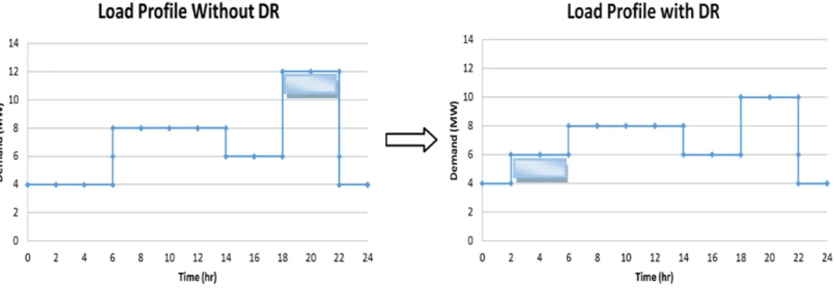
When the load is apparently higher than the average level in a certain period, a certain amount of load must be moved from that period to other periods. It primarily relies on the deferrable appliances, which can justify the time of usage, e.g., washing machines. In the short term, load shifting can be achieved on a daily basis from peak time to off-peak time. Fig. 2.3 shows a daily load shifting in which part of the peak demand is shifted from 18:00-20:00 to 2:00-6:00. It does not reduce the total consumption, but only changes the time of usage.

Figure 2.3: Demonstration of load shifting.

Strategic conservation

When the overall load exceeds the supply level, customers are encouraged to reduce the overall consumption. One basic method is to improve the energy efficiency. It can be applied at a small scale by replacing traditional devices with energy-efficient devices, e.g., changing filament lamps to fluorescent lamps. It also can be applied at a large scale, e.g., weatherization program, which is aimed to reduce the energy bill for low-income families by improving the energy efficiency of their house [29]. Besides the technical improvements, the information supports are also important. In general, providing consumption and cost details to customers can facilitate the power reduction. Fig. 2.4 shows strategic conservation from a high power level to a low level.

(35)

Figure 2.4: Demonstration of strategic conservation.

Strategic load growth

When the demand falls below the normal level of supply, customers are encouraged to increase the overall consumption. The electrification technology has the potential for this service, e.g., the popularization of electric vehicles. Fig. 2.5 shows strategic load growth from a low power level to a high level.

Figure 2.5: Demonstration of strategic load growth.

2.4.3 Customers category

DR is primarily focused on the Customers side. Detailed analysis of customers can facilitate the understanding and design of it. Generally, customers can be classified into four sectors: 1) Industrial sector; 2) Residential sector; 3) Commercial sector and 4) Transportation sector [30]. Fig. 2.6 shows the portion of electricity

(36)

con-2.4. Demand Response 16 sumption about each sector in the U.K. in 2017. As for the DR, industrial sector, residential sector and commercial sector are mainly concerned.

Figure 2.6: The electricity market share by sectors in the U.K. in 2017 [29].

Residential sector

The usage patterns in the residential sector are more complicated than the other two. Firstly, the quantity of customers is much higher. The distribution of customers is wide and scattered. Secondly, the types of appliances used by customers are diverse. Even for the same type of appliances, the power consumption of different brands can vary. Thirdly, every customer has his or her own personal preference of usage. That means each customer needs to be treated specifically rather identically [31].

Customers can be divided into five types based on the rationality [32]: 1) Long-range customers: their elasticity of electricity is relatively high. They are able to modify the usage in a wide range of time. 2) Real world-postponing customers: they consider the current and future electricity prices, and give certain responses to utilities. 3) Real world-advancing customers: they focus on the past and future electricity prices, and also give certain responses to utilities. 4) Real world-mixed customers: they are a combination of both postponing customers and advancing cus-tomers. 5) Short-range customers: they only pay attention to the current electricity price. Therefore, they are not willing to change their consumption pattern.

(37)

2.4. Demand Response 17 Industrial sector

It has a high electricity consumption, especially at a high voltage level. In addition, the peak load of it is significant. However, the adaption of DR in this sector is challenging [33]. Firstly, the information of the usage pattern and the operation of the appliances is confidential in some cases. To some extent, It can reflect the process of the manufacture, which is classified in a few industries. Therefore, the access to this information is limited. Secondly, even if there is sufficient information, the modification of electricity usage is still tough because many procedures are time-sensitive. They require a precise order and duration, which means they are less likely to be shifted. In this situation, a proper choice for industries is to improve the energy efficiency.

Commercial sector

The usage pattern in the commercial sector is quite typical and identical. The common and main loads for commercial customers come from the use of heating, ventilation, air-conditioning systems and lighting systems. The modification of these systems is relatively easy. Firstly, in general, these systems are autonomously con-trolled according to the preset requirements. This makes the systems able to quickly respond to the DR signals. Secondly, the effect of the external factors, e.g., temper-ature, humidity, and illumination, to these systems are predictable. For example, a light system consumes more electricity in winter than in summer [34].

Among these three sectors, the commercial sector and the industrial sector are relatively easier to realize the DR programs. Commercial and industrial customers are distributed regionally and intensively, and the power consumption of these cus-tomers is relatively high. What’s more, the appliances and control systems for these customers are more advanced. In addition, in case of the emergency, most of these customers are equipped with the backup on-site generator. These appliances also can be used as auxiliary facilities of the DR programs [35]. Furthermore, the commercial and industrial sectors have a larger capacity of potential peak load reduction [36].

(38)

2.4.4 Loads category

Based on the operation characteristics of appliances, the loads can be classified by two standards: 1) whether the occupied time duration of appliances can be modified or not; 2) whether the total electricity consumption of appliances can be modified or not. For the first standard, loads can be divided into deferrable loads and non-deferrable loads [37]. For the second standard, loads can be divided into adjustable loads and nonadjustable loads [38].

Deferrable loads and non-deferrable loads

The activation time of deferrable loads can be stopped, re-started, and shifted to other time slots, e.g., washing machine and electric vehicles. Generally, most of the wet loads belong to the deferrable loads. These loads can be scheduled by a DR program. Based on the electricity price or the monetary incentive, they can be shifted from peak-hour to off-peak hours, therefore reducing the peak load demand [32]. The modification of these loads needs to abide by the predefined requirements, e.g., deadlines and operation times. On the contrary, the non-deferrable loads need to finish the schedule at specified time, e.g., lighting systems and kitchen systems [39]. These loads do not allow the time shift and interruption. As such, these loads are not suitable for the DR program.

Adjustable loads and nonadjustable loads

For the adjustable loads, the consumption can be adjusted to a lower level, e.g.,

in winter heaters can be set at 23o_{C rather than 25}o_{C [40]. Normally, most of}

the thermal loads are part of the adjustable loads. These loads can be involved in the DR program. The total consumption can be brought down on the base of electricity price or the monetary incentive. However, reducing the consumption can affect customers’ comfortability described by the quality of experience (QoE) [41]. QoE refers to the valuation of customers’ experiences or satisfaction degree during a service. When a DR program is designed, this QoE must be taken into consideration to make sure that the DR program is executable theoretically and practically [42]. In contrast, for the nonadjustable loads, the total consumption is settled, e.g., TVs

(39)

2.4. Demand Response 19 and computers [43]. Same as the non-deferrable loads, nonadjustable loads cannot be scheduled by a DR program either.

2.4.5 Approaches category

There are a number of motivation methods that encourage customers to participate in a DR program. These methods can be divided into two groups: time-based DR and incentive-based DR [44, 45].

Incentive-based DR

In these methods, incentives are offered to customers depending on their behaviour in the DR programs. Normally, customers are voluntary to change their consumption. However, in some cases, the failure of meeting the requirements will result in a penalty for customers. Generally, there are five types of incentive-based DR [46]: 1) Direct load control; 2) Interruptible/Curtailable service; 3) Demand bidding; 4) Capacity market program and 5) Ancillary service market .

• Direct load control: According to the advanced agreement between customers

and utilities, utilities can remotely control some customers’ appliances, e.g., air-conditioners and water heaters. The notices of the operation are normally announced at a short time ahead. To participate in this method, customers need to be equipped with a remote control switch system so that utilities can shift, turn on or turn off the appliances [47]. Direct load control is primarily applied to the residential sector or small-scale commercial sector. It is not suitable for the industrial sector because the industrial sector needs a precise process.

• Interruptible/Curtailable service: Compare to the direct load control, this

method is normally applied to the industrial sector and large-scale commer-cial sector. When the system is congested, customers are asked to reduce some loads to a certain level. By participating in it, customers can receive a rate discount or bill discount. However, if customers failed to respond in the

(40)

2.4. Demand Response 20 predefined time period, they could receive a penalty [48]. In this method, the operation frequency and the duration are limited.

• Demand bidding: Instead of being asked by the utilities to take part in the DR

programs, customers can make decisions by themselves in this method. Based on the generation and demand situation, utilities announce the total amount of electricity that must be curtailed. Customers can bid for the amount based on their own situation and wholesale market. Once the bid is accepted, they must provide the specified curtailment, otherwise, they will get the penalty [49]. This method is also suitable for large-scale customers. For small-scale customers, they can be integrated by aggregators and involved in as a unity.

• Capacity market program: When the system is short of the reserve, customers

are required to reduce the pre-defined consumption. The announcement is normally released one day ahead. These curtailments are treated as system capacity to replace the conventional generation and delivery resources. By proving the ability for the curtailment, customers can get reservation payment. And by providing the reduction, customers can get an incentive. In contrast, if they failed to provide it, they could receive a penalty [46].

• Ancillary service market: Similar to the demand bidding, customers also bid

for the electricity curtailments. These bids are offered to independent system operator/regional transmission organization [46]. These curtailments are used as the operational reservation. If the bid was accepted, customers need to abide by a standby standard. In this situation, they are paid by the market price. Once the curtailments are really called, customers are paid by the spot price.

Time-based DR

In these methods, electricity prices vary according to the cost of generation and demand of electricity. Based on these prices and other information, customers can decide their consumption. Generally, there are four types of pricing schemes [35]:

(41)

2.4. Demand Response 21 1) Flat pricing; 2) Time-of-use (ToU) pricing; 3) Critical peak pricing and 4) Real time pricing .

• Flat pricing: This is the most traditional and widely used price scheme. The

electricity price is constant all the time. In this situation, the only way to reduce the bill is to reduce the total consumption. The prices can be designed seasonally. Within a season, it is fixed. And for another season, a different price is used.

• ToU pricing: It is an improvement from flat pricing. The prices are different

in different time slots. Within each slot, a flat price is applied. Fig. 2.7 shows an example of ToU pricing. Usually, prices are pre-defined for one day [35]. In this scheme, customers tend to shift their demand to a lower price period. In this way, the ability to reduce the total electricity demand is narrowed. For example, in the U.K., an Economy 7 tariff is applied in some area. It offers a cheap electricity price for the off-peak time, typically the night. This off-peak time lasts 7 hours in total, as the “7” implied, normally from 0:00 to 07:00. The price for day-time is higher, around 13-16p per kWh, while the price for night-time is lower, around 5-7p per kWh. This tariff was first introduced in 1978. To apply for the Economy 7, customers need to be equipped with a particular meter that can show two different readings: one for day-time electricity consumption and the other for night-time electricity consumption.

• Critical peak pricing: This scheme is derived from the ToU pricing scheme.

The extreme peak demand period is picked out. During this period, a much higher electricity price is announced [31]. Fig. 2.8 shows an example of critical peak pricing. This scheme can effectively bring down the peak demand [31]. The critical peak price can be designed by the demand level or the time of the day. Three types of pricing are considered: fixed-period critical peak pricing, variable-period critical peak pricing and variable critical peak pricing. For fixed-period critical peak pricing, a specific period in one day is selected and a fixed high electricity price is applied based on the experience accumulation. For variable-period critical peak pricing, the application period is not fixed. The

(42)

Figure 2.7: Demonstration of ToU pricing.

utilities can choose to trigger the critical peak pricing based on the pre-defined criteria. In this situation, the operation frequency and duration are limited. For variable critical peak pricing, the period is fixed, but the electricity price can vary on the basis of the current demand situation [50].

Figure 2.8: Demonstration of critical peak pricing.

• Real time pricing: The electricity price fluctuates frequently, normally by

hours. Fig. 2.9 shows an example of real time pricing. The change of price can indicate the relationship between supply and demand in the wholesale market [51]. It requires effective two-way communication between utilities

(43)

2.5. Review of the Existing Theories, Models, and Methodologies 23 and customers. Sometimes, market aggregators also take part in this scheme to deal with the data collection and speed up the efficiency. Customers are involved mostly in this scheme and notified of these prices in a day-ahead man-ner, hour-ahead manner or 15-minutes ahead manner. Based on the price and the own situation, customers can decide their consumption pattern. Based on the total generation situation, total demand situation and customers reactions for the former price, utilities can decide the prices for the next period. This scheme is more acceptable by the industrial and commercial sectors than by the residential sector. There are two main difficulties for the application of this scheme. Firstly, it relies on continuous real-time data exchange, which is not favorable for customers [35]. Secondly, the large-scale data processing increases the complexity of the whole system [44].

Figure 2.9: Demonstration of real time pricing.

2.5 Review of the Existing Theories, Models, and

Methodologies

In this section, state-of-the-art models and methodologies are reviewed. The role of DR aggregator in electricity market is introduced at first. Then, the economic and environmental scheduling of electricity generation is presented. After that, the carbon emission tracing in power system is provided.

(44)

2.5. Review of the Existing Theories, Models, and Methodologies 24

2.5.1 Demand response aggregator in electricity market

Although the development of DSM has a great future, the application of it is still a challenging task. If the generation side directly communicates with customers, there will be numerous information exchanges, which can delay the system response time. Meanwhile, the generation side is designed for large scale. The effect of individual’s pattern is almost negligible to the system. The generation side is not able to negotiate directly with each customer. In this context, an intermediary/ representative is needed [52, 53].

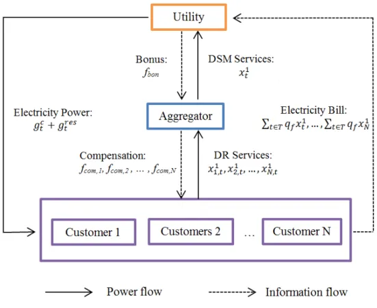
Figure 2.10: Functionality of the DR aggregator in a power grid [54].

Aggregator, as the name implies, bundle a group of customers into a cluster, therefore becomes an important aspect to the grid and occupies a certain weight in the trade [54]. As shown in Fig. 2.10, DR aggregator can bring several benefits into the system [55]. For distribution system operators (DSOs), it can achieve

(45)

peak-2.5. Review of the Existing Theories, Models, and Methodologies 25 load shaving and distributed generation (DG) supply optimization; For retailers, it can help with the internal portfolio balancing; For the market, it can deliver day-ahead/hour-ahead optimization, frequency control and power reservation [56,57]. In the U.K., DR aggregator is a booming entity. It is allowed and supported by the government in the power network. There are already many DR aggregators exist in the market from different companies, e.g., U.K. Power Reserve Ltd; KiWi Power Ltd; Npower Ltd; ESP Response Ltd [58].

The interactions between the generation side and the DR aggregator can be categorised into two different types:

• Mutual interaction: The network information is provided by the generation

side in advance, DR aggregator then acts as a retailer buying electricity energy in the day-ahead market biding on the bulk and price of it.

• Directed interaction: The generation side announces that power adjustment

re-quirement in the particular time slot, DR aggregator then attempts to achieve the goal, and if so, being rewarded by the generation side.

To introduce the aggregator into the system, a two-stage market model was proposed in [59]. For the first stage, the utility acted as the leader, setting the price for buying a certain power capacity from aggregators at particular time slot. Aggregators acted as followers, determining the supply capacity. The tatonnement process was used to achieve the equilibrium. For the second stage, aggregators acted as leaders, setting the price for buying power capacity from customers. Customers acted as followers, determining the supply capacity. The supply function bidding was used to maximize aggregators’ profit. This work was designed for a certain time period and mainly focus on the aggregators’ side.

In [60–63], the time horizon was extended. The dynamic electricity price over time was implemented in [60, 61]. The aggregator would give rewards to customers if they schedule their appliances according to the signal. The appliances were cate-gorized into shiftable loads, thermal loads and interruptible loads. A mixed integer linear programming and a heuristic allocation algorithm were proposed to maximize aggregators’ profit [60], and minimize the overall energy cost while considering

(46)

cus-2.5. Review of the Existing Theories, Models, and Methodologies 26 tomers’ QoE [61]. The critical peak pricing was applied in [62]. The aggregator decided the time to employ the critical peak price. The regulatory, economic and technical perspectives of critical peak price were examined. In [63], the aggregator coordinated the regulation service on supply side and the DR service on consumer side. The regulation service could have a frequent control but a relatively slow up-date, while the DR service could have a quick response but could not change the control repeatedly. A multi-rate model predictive control approach was used to the capture the imbalance. When the imbalance occurred, an indirect signal was given, and then the DR aggregator solved a quadratic problem at each time slot.

In [52, 64, 65], a layered settlement mechanism was proposed. In [64], the inde-pendent system operator was at the first layer, announcing the power curtailment requirement in advance. The aggregator was at the second layer, committing to achieve the target. Customers were at the third layer, bidding their ancillary ser-vices to the aggregator. With the precondition of meeting the curtailment require-ment, the mechanism aimed at minimizing customers’ supply function, that is the incurred disutility minus the compensation. The model in [52] included the utility, DR aggregators, and customers. The utility provided rewards to aggregators for providing DR services, and customers can receive monetary compensation from DR aggregators for their demand adjustment. In [65], the aggregator was an agent, com-municating with transmission system operator and residential storage space heating. It helped customers to minimize the electricity payment and maximize the bonus.

In [66, 67], the concept of virtual power plant was mentioned, which gathering distributed energy resources (DERs) to make them more manageable when partic-ipating in the real-time operating system. In [66], a direct load control approach was applied to schedule thermostatically controlled appliances in the virtual power plant, for the purpose of minimizing the demand. The aggregator bided the load reduction capability to electricity market, assisting the reduction of congestion and deviation between generation and demand. In [67], the aggregator provided services to the primary and secondary reserve markets. It could continuously modify the operation schedule of appliances to maximize the portfolio. This could solve the restriction issues of energy limitations and inaccurate baselines information in the

(47)

2.5. Review of the Existing Theories, Models, and Methodologies 27 virtual power plant.

In [68], the aggregator provided variety of DR strategies for consumers and DR service punchers. The aim of the aggregator was to maximize its profit. For cus-tomers, the aggregator implemented a ToU electricity price and a stepwise reward price for the load reduction. For DR service purchasers, the aggregator offered a fixed DR contract and an optional DR agreement. In fixed DR contract, the aggre-gator would provide a certain amount of load curtailment for a given time period. In optional DR agreement, the aggregator would provide the service only if it is profitable. The case study on the Australian national electricity market showed that the uncertainty on power consumption had a significant effect on the strategy, and should be considered. Therefore, the research in [69] took this uncertainty into consideration, a wind power offering strategy was proposed. A bi-level problem was formulated. The decision maker for the upper-level problem was wind power pro-ducer, setting its DR price. The decision maker for the lower-level problem was the DR aggregator, determining its market share. This problem is then linearised into a single level problem and be solved. And in [70], uncertainties were detailed classified, that caused by power demand, customers preferences, external environ-mental conditions, house thermal requirements and wholesale market. The Monte Carlo simulation method was applied to model these uncertainties. The DR aggre-gator represented customers to bid energy in the market. Customers were willing to modify their consumption profile according to the electricity price, in which the distribution locational marginal price in a real-time distribution market was used.

In [71–73], multiple utilities were involved, and the role of DR aggregator that balances the generation and demand was studied. Utilities aimed to maximize the profit, while customers aimed to maximize their individual welfare. A Stackelberg game was established based on that to solve the problem. In [73], utilities were divided into two types, fossil-fuel based and RESs based. The uncertainty of supply was considered. A utility selection program which can minimize customers’ costs was proposed.

(48)

2.5. Review of the Existing Theories, Models, and Methodologies 28 Research Challenges

In [61, 64, 65], only the objective for customers was considered. In [62, 63, 67, 70], the role of the DR aggregator was involved, but the utility function was not explicit. Only benefits for the generation side and the customer side were considered, while the benefit for the DR aggregator was neglected. In [52, 60, 64, 70], only the conven-tional generation was considered. In [66, 71–73], the inconvenience caused by DR program for customers was not detailed. A day-ahead demand planning with DR aggregators integrating RESs is proposed in Chapter 3 to address these challenges.

2.5.2 Economic/Environment scheduling of electricity

gen-eration

The fuel source scheduling of electricity supply plays an important role in the sus-tainable development. The analysis of fuel sources usage of electricity generation can elementally mitigate the carbon emission from the very beginning. A great num-ber of researches were carried out on that [74–76]. Fig 2.11 illustrates the general structure of fuel source scheduling problems [77, 78].

In the beginning, only the economic scheduling of generation was considered. It was used to dispatch the committed generators’ outputs so as to meet the load demand most economically. It mainly focused on minimizing the generation cost or maximizing the generation profit under variety system operation constraints. Amount of approaches were introduced, such as non-linear programming [79], se-quential quadratic programming [80], hierarchical decentralized method [81], particle swarms algorithm [82] and genetic algorithm [83].

However, with the rising concerns of climate change and air pollution, the simplex consideration of economic scheduling was not enough. Utilities were requested to gradually reduce the carbon emission from power plants [84, 85]. Diverse strategies were proposed and discussed for the environmental protection, such as installing post combustion cleaning equipment, switching to low emission fuels, replacing the aged fuel burners with cleaner ones, and emission dispatching [86]. The most direct way to quantify and regulate the carbon emission in electricity generation was the

(49)

2.5. Review of the Existing Theories, Models, and Methodologies 29

(50)

2.5. Review of the Existing Theories, Models, and Methodologies 30 last strategy. The pure emission scheduling was similar to the economic scheduling, with the objective to be minimized being emission instead of generation cost. But still, this approach was onefold for the system.

The basic way to take both economic and environmental aspects into consid-eration was to set the carbon emission as a constraint for the scheduling problem, which leads to an emission constrained economic scheduling problem [87–89]. In [87], the total generation cost was minimized with a pre-specified carbon emission limit. In [88], two scenarios were analysed. The first scenario modelled cost function in a quadratic form. And the second scenario modelled cost functions in the form of quadratic summed with a sine term, in order to incorporate the valve-point effect for actual power system operation. The second scenario showed a higher cost than the first one. In [89], the total generation profit was maximized while fulfilling elec-tricity demands and carbon emission mitigation. The financial risk of uncertainties, i.e. carbon emission mitigation operating costs, carbon credit prices and electricity prices, were imposed to the objective function by a penalty factor. The case study suggested replacing petroleum-fired power plants with coal-fired ones in Korea. And nuclear plants showed a great potential for the future market. But these work only took the carbon emission as a constraint, therefore can not reveal the relationship between generation cost and carbon emission.

Another simple way to involve both economic and environmental aspects was to combine these two objectives into one single objective, which brings the concept of environmental/economic scheduling. In [90–92], these two objectives were linearly combined. In [92], the emission constrained economic scheduling problem was com-pared with the economic emission scheduling problem. In the second problem, the total carbon emission was taken as an individual objective. For the first problem, as the total carbon emission allowance increased, the total power generation and profit were increased. For the second problem, an emission control cost factor was introduced to assign the weight between emission function and fuel costs function. As the importance of carbon emission increased, the total power generation and profit were decreased. However, in these approaches, the priori weight/preference need to be given between the generation cost and carbon emission.

Decarbonising Future Power Systems by Demand Side Management in Smart Grid

Durham E-Theses

Decarbonising Future Power Systems by Demand Side

Management in Smart Grid

Decarbonising Future Power Systems

by Demand Side Management

in Smart Grid

Dan Li

A Thesis presented for the degree of

Doctor of Philosophy

Department of Engineering

University of Durham

United Kingdom

August 2018

Decarbonising Future Power Systems by Demand

Side Management in Smart Grid

Dan Li

Abstract

Declaration

Acknowledgements

Publication List

Book Chapter

Journal Paper

Conference Paper

Contents

List of Figures

List of Tables

List of Symbols and Abbreviations

Chapter 1

Introduction

1.1

Background

1.2

Research Motivations

1.3

Research Objectives

1.4

Research Contributions

1.5

Thesis Outline

Chapter 2

Literature Review

2.1

Introduction

2.2

Smart Grid

2.3

Demand Side Management

2.3.1

Definition

2.3.2

History

2.3.3

Advantages

2.4

Demand Response

2.4.1

Definition

2.4.2

Services category

2.4.3

Customers category

2.4.4

Loads category

2.4.5

Approaches category

2.5

Review of the Existing Theories, Models, and

Methodologies

2.5.1

Demand response aggregator in electricity market

2.5.2

Economic/Environment scheduling of electricity

gen-eration