Time Preferences And Risk Aversion:
Tests On Domain Differences
Christos A. Ioannou
∗†Jana Sadeh
‡This draft: December 26, 2014
Abstract
The design and evaluation of environmental policy requires the incorporation of time and risk elements as many environmental outcomes extend over long time periods and involve a large degree of uncertainty. Understanding how individuals discount and evaluate risks with respect to environmental outcomes is a prime component in designing effective environmental policy to address issues of environmental sustainability, such as climate change. Our objective in this study is to investigate whether subjects’ time preferences and risk aversion across the monetary domain and the environmental domain differ. Crucially, our experimental design is incentivized: in the monetary domain, time preferences and risk aversion are elicited with real monetary payoffs, whereas in the environmental domain, we elicit time preferences and risk aversion using real (bee-friendly) plants. We find that subjects’ time preferences are not significantly different across the monetary and environmental domains. In contrast, subjects’ risk aversion is significantly different across the two domains. More specifically, subjects (men and women) exhibit a higher degree of risk aversion in the environmental domain relative to the monetary domain. Finally, we corroborate earlier results, which document that women are more risk averse than men in the monetary domain. We show this finding to, also, hold in the environmental domain.
JEL: C51, C91, D03, Q05
Keywords: Discounting, Risk Aversion, Domain Differences, Environmental Domain
∗The usual disclaimer applies.
†Mailing Address: Department of Economics, University of Southampton, Southampton, SO17 1BJ, United Kingdom.
Email: [email protected]
‡Mailing Address: Department of Economics, University of Southampton, Southampton, SO17 1BJ, United Kingdom.
1
Introduction
The design and evaluation of environmental policy requires the incorporation of time and risk elements as many environmental outcomes extend over long time periods and involve a large degree of uncertainty. Understanding how individuals discount and evaluate risks with respect to environmental outcomes is a prime component in designing effective environmental policy to address issues of environmental sustainability, such as climate change. Our objec-tive in this study is to investigate whether subjects’ time preferences and risk aversion across the monetary domain and the environmental domain differ. By domain, we refer to the set to which a particular measurement instrument belongs (i.e. choices over outcomes measured in money belong to the monetary domain, whereas choices over outcomes measured in, say, plants belong to the environmental domain).
We elicit subjects’ time preferences and risk aversion using a controlled ‘within-subject’ experimental design. First, to isolate the effect of domain on intertemporal choices, the fixed-sequence choice titration (Harrison and Lau (2005); Read, Frederick, Orsel, and Rahman
(2005);Andersen, Harrison, Lau, and Rutstr¨om(2008);Hardisty and Weber(2009)) is used. In this approach, subjects are presented with a series of binary intertemporal choices between a fixed amount that is due at one point in time (henceforth, referred to assmaller sooner) and a larger amount that is due at a later point in time (henceforth, referred to as larger later). While the smaller sooner amount is kept fixed, the larger later amount increases successively. In the beginning, subjects typically prefer the smaller sooner amount to the larger later one. However, at some point, a switch takes place from the smaller sooner to the larger later amount, which enables the experimenter to extract the discount-rate bracket within which the individual’s rate of time preference lies. Second, to elicit subjects’ risk aversion, a variant of the Eckel-Grossman test (Eckel and Grossman (2002); Eckel and Grossman
(2008)) is used, where subjects are presented with five gambles of varying riskiness and are required to select the one they prefer. Crucially, in order to ensure that the magnitude of the choices in the monetary domain matched those in the environmental domain, prior to running the experimental sessions, we calibrated the value of the environmental instrument using two contingent valuation studies. Finally, subjects were required to take the Cognitive Reflection Test and to complete a questionnaire. The latter two tasks enabled us to obtain both a measure of subjects’ cognitive ability to reflect and deliberate in the face of intuitively simple alternatives as well as insights to subjects’ environmental attitudes, which could possibly relate to the way different domains were evaluated.
A novelty of the experimental design is that it is incentivized: in the monetary domain, time preferences and risk aversion are elicited with real monetary payoffs, whereas in the
environmental domain, we elicit time preferences and risk aversion using real (bee-friendly) plants.1 Our choice for the appropriate environmental instrument was not an easy one. The
instrument had to be familiar to subjects to facilitate their understanding of its potential benefits, and credible so that subjects could rest assured that the project is one that can be easily implemented without arousing suspicion of deception. Finally, the instrument had to be divisible so as to enable us to vary the larger later amount and the gambles. The choice of a locally-based project that distributed bee-friendly plants fulfilled all these requirements.2
Our first set of main results does not find any significant differences in subjects’ time pref-erences across the monetary and environmental domains. Assuming away any philosophical or ethical issues that might dictate what the discount rate ought to be in environmental cost-benefit analysis, a corollary of the first result is that the same discount rate used for financial payoffs should also be used for the environmental ones when evaluating environ-mental policies. This corollary is reassuring to economists and policy makers who, for some time now, have been evaluating environmental policies with discount rates that are based on the intertemporal-choice framework of the monetary domain.
Our second set of main results finds domain differences in subjects’ risk aversion. More specifically, subjects (men and women) exhibit a higher degree of risk aversion in the en-vironmental domain relative to the monetary domain; that is, individuals tend to be more reluctant to take on large gambles with environmental outcomes than with monetary ones. A plausible explanation for the emergence of domain differences in risk aversion could be stemming from individuals’ perception on the consequences of climate changes−a topic that has been well publicized. Furthermore, we corroborate existing results, which document that women are more risk averse than men in the monetary domain. We show this finding to, also, hold in the environmental domain. The latter findings seem to hint that women are more risk averse than men independently of the domain, although more research is necessary to validate such conjecture.
Our third set of results does not find any support of the hypothesis that time prefer-ences/risk aversion are correlated with subjects’ cognitive abilities or environmental aware-ness. However, when we partition the discounting behavior of subjects into three categories based on whether they discounted the environmental domain the same as, more than, or less than the monetary domain, we find significant correlation between subjects exhibiting environmental awareness and lower discounting in the environmental domain.
1There exists evidence to suggest that incentivized experiments may have an impact on the discount rates elicited (Coller and Williams(1999);Kirby and Marakovi(1995)).
2To the best of our knowledge, this is the first study to use a real environmental instrument; the only other study that we are aware of that investigates differences in time preferences across the monetary and the environmental domains used hypothetical environmental payoffs (Hardisty and Weber(2009)).
The paper adheres to the following plan. We present next an overview of the related literature. Section 3 describes, in relative detail, the experimental design. Section 4 presents the data analysis, and Section 5 discusses the important findings and provides direction for future research.
2
Literature Review
Our paper is related to two main strands of the literature on decision-making across domains. First, it is related to the growing literature on domain differences in time preferences. The impact of domains on intertemporal choice has predominantly revolved around the monetary domain and the health domain, where most studies find differences in subjects’ discounting behavior.3 Recently, in the midst of a public debate on the appropriate discount rate to evaluate the consequences of climate change (Stern (2007); Nordhaus (2007)),4 the investi-gation on the impact of domains on intertemporal choice has expanded to, also, include the environmental domain. In their study, Hardisty and Weber (2009) compared intertemporal choices elicited in the three aforementioned domains and found that subjects’ discounting behavior was not statistically different across the environmental and monetary domains, but was statistically different across the health domain and the other two domains. Hardisty and Weber(2009) attributed the domain effect in health to subjects’ visceral reaction to the health scenarios. Other studies have also assessed the discounting behavior of subjects in the environmental domain albeit via risk assessments. B¨ohm and Pfister (2005), for exam-ple, conducted experiments to measure subjects’ risk assessment of hypothetical scenarios on coastal erosion and marine oil spills. The authors found that temporal discounting of environmental risks was weak and postulated that ethical evaluations were not discounted by subjects. Along the same lines, Gattig and Hendrickx (2007) concluded that temporal discounting was less pronounced for environmental risks than for risks in other domains. Finally, Viscusi, Huber, and Bell (2008) estimated discounting rates based on a series of environmental policy choices administered in a survey context. A key finding of their study was that discounting behavior differs markedly for people who visit lakes, rivers, and streams for recreational purposes and those who do not. More specifically, regular visitors to water 3Many studies find that discount rates in the health domain are larger than those in the monetary domain for health gains, but lower than those in the monetary domain for health losses (Cairns (1992); Chapman and Elstein(1995);Madden, Bickel, and Jacobs(1999)).
4As Weitzman(2007) aptly notes, “it is not an exaggeration to say that the biggest uncertainty of all in the economics of climate change is the uncertainty about which interest rate to use for discounting” (p. 705).
bodies have low discounting rates, whereas those who do not visit water bodies often have consistently high discounting rates.
Our work is also related to the literature on risk preferences across domains. Dohmen, Falk, Huffman, Sunde, Schupp, and Wagner(2011) used a large, representative survey of the German population to elicit risk preferences across a number of domains and found that the self-reported risk-taking measures are highly, but not perfectly, correlated across domains.5
In a study with a different flavor, Riddel (2012) compared subjects’ evaluation of financial and environmental lotteries to determine whether preferences over environmental risks can be reasonably approximated by the Expected Utility framework. The author found that subjects were more likely to overemphasise low probability, extreme environmental outcomes than low probability, extreme financial ones. As a result, she concluded that the Expected Utility framework is likely to underestimate subjects’ willingness to pay for environmental cleanup programs or policies with uncertain outcomes. Much earlier,Weber, Blais, and Betz
(2002) argued that individuals are not characterized by a single risk attitude, but rather exhibit different risk preferences depending on the domain.
All the aforementioned studies pertaining the environmental domain used an elicitation method based on hypothetical environmental gains and losses. In sharp contrast, our study uses an incentivized scheme with real monetary and environmental payoffs. The use of real payoffs creates a strong incentive for subjects to display their true preferences and increases the attention given to the task at hand. There is evidence that the use of real payoffs might matter in discounting experiments. For instance, Kirby and Marakovi (1995) found that discount rates elicited for real monetary payoffs were higher than those elicited for hypothetical ones. Testing a similar setting,Coller and Williams(1999) were less conclusive in their findings, while Camerer and Hogarth (1999), in a wide survey on the role of real incentives, found no effect on mean performance albeit found a reduction in variance with high financial incentives. The authors noted that high incentives improved performance in demanding tasks and reduced generosity and risk-seeking behavior. The effect of incentives is, also, confirmed in other studies investigating the impact of real payoffs in experiments (Kroll, Levy, and Rapoport (1988); Cummings, Harrison, and Rutstr¨om (1995)).
5Dohmen, Falk, Huffman, Sunde, Schupp, and Wagner(2011) tested the following domains: career choices, leisure and recreational activities, financial decisions, health, and driving. They used a scale from 1 to 10, with 10 signifying the greatest willingness to take risks.
3
Experimental Design
Our experimental setup featured six tasks. Two of these tasks aimed to investigate subjects’ intertemporal choices across the monetary domain and the environmental domain. The two tasks differed solely on the instrument that was discounted; that is, the valuation of the two instruments was identical (see Subsection3.2). In the monetary domain, the instrument that was discounted was money, whereas in the environmental domain the instrument that was discounted was plants. To isolate the effect of domain on intertemporal choices, we used the fixed-sequence choice titration (Harrison and Lau (2005); Andersen, Harrison, Lau, and Rutstr¨om (2008); Hardisty and Weber (2009)).6 In this approach, subjects are presented
with a series of binary choices between a fixed amount that is due at one point in time and a larger amount that is due at a later point in time. While the smaller sooner amount is kept fixed, the larger later amount increases successively. The experimental data on the repeated binary intertemporal choices are transformed into a single switching point; the latter produces a discount-rate interval, which contains the indifference point of each subject. Another two tasks aimed to measure the risk aversion of subjects across the monetary domain and the environmental domain. The tests on risk aversion were based on the Eckel-Grossman test (Eckel and Grossman (2002); Eckel and Grossman (2008)) and differed, only, on the measurement instrument. Analogous to the previous setup, in the monetary domain, the test used monetary gambles, whereas in the environmental domain, the test used gambles in plants. In addition to the four aforementioned tasks, subjects were required to take the Cognitive Reflection Test (CRT) and to complete a questionnaire. On one hand, the CRT allowed us to obtain a measure of subjects’ cognitive ability to reflect and deliberate in the face of intuitively simple alternatives. On the other hand, the questionnaire allowed us to elicit subjects’ environmental attitudes.7 In summary, the addition of the latter two tasks served to provide insights into possible individual heterogeneity that could be related to the way different domains were evaluated by subjects.
6Other studies (Raineri and Rachlin (1993); Green, Fry, and Myerson (1994)) have used the staircase choice titration method. The latter method presents subjects with an initial binary intertemporal choice and dynamically adapts the subsequent choices depending on the subject’s decisions. Finally, a third method is the matching-tasks method (Kirby and Marakovi(1995);Chapman(1996);Cairns and van der Pol(1999)), where subjects are asked to indicate what amount they would require in order to postpone the receipt of a given outcome by a given time delay. In essence, this method asks subjects to reveal directly the upper bracket of their indifference point. However, Hardisty, Thompson, Krantz, and Weber (2013) note that choice-based measures, such as the fixed-sequence choice titration and the staircase choice titration, are better predictors of real world outcomes than matching tasks. Additionally, the authors point out that the demanding dynamic staircase titration offers no advantages over the simpler fixed-sequence choice titration, making the latter the most appropriate method for this experiment.
7The questions were taken from the Segmentation Model created by the Department for Environment, Food & Rural Affairs (DEFRA(2008)).
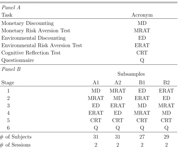
Our experimental design applied a hybrid of a ‘within-subject’ and ‘between-subject’ design (Charness, Gneezy, and Kuhn(2012)). In line with a standard ‘within-subject’ design, each subject was exposed sequentially to the six tasks. We safeguarded against the possibility of observing order effects by splitting the sample into four subsamples (A1, A2, B1 and B2). The four subsamples differed only in the order the first four tasks were presented (i.e. the monetary discounting task, the monetary risk aversion test, the environmental discounting task, and the environmental risk aversion test), thereby replicating a ‘between-design’ for these four tasks. This allowed us to harness the strength of each design while safeguarding against possible confounds. The experimental design is indicated in Table 1. In Panel A, we provide a brief description of the task and the corresponding acronym. In Panel B, we display the order of the tasks in the four subsamples.
Table 1: Experimental Design
Panel A
Task Acronym
Monetary Discounting MD
Monetary Risk Aversion Test MRAT
Environmental Discounting ED
Environmental Risk Aversion Test ERAT
Cognitive Reflection Test CRT
Questionnaire Q Panel B Subsamples Stage A1 A2 B1 B2 1 MD MRAT ED ERAT 2 MRAT MD ERAT ED 3 ED ERAT MD MRAT 4 ERAT ED MRAT MD 5 CRT CRT CRT CRT 6 Q Q Q Q # of Subjects 31 31 27 29 # of Sessions 2 2 2 2
Notes: In Panel A, we provide a brief description of the task and the corresponding acronym. In Panel B, we display the order of the tasks in the four subsamples. The last 2 tasks were common in all four subsamples. The first four tasks (MD, MRAT, ED and ERAT) were shuffled across the four subsamples. The last two rows, display the total number of participants and the number of sessions in each subsample.
3.1
Environmental Instrument
Our choice for the appropriate environmental instrument was not an easy one. First, we required that the instrument is divisible so as to enable us to vary the larger later amount and the gambles. Second, the instrument had to be familiar to subjects and credible. It had to be familiar to subjects to facilitate their understanding of its potential benefits as well as credible so that subjects could rest assured that the project is one that can be easily implemented without arousing suspicion of deception. The choice of a locally-based project that distributed bee-friendly plants fulfilled all these requirements. Subjects were instructed that bee-friendly plants would be handed out to staff and students on campus to be placed in outdoor areas. Given the different delay periods, different bee-friendly plants were chosen. Subjects were informed that the plants distributed would be chosen depending on the season to ensure that they are immediately beneficial.
The environmental project was described in a succinct and neutral manner. The link between bee-friendly plants and the positive externality they generate was stated in the description as well as the fact that bee populations are in decline. These two facts are central to the placing of the project as an environmentally beneficial one. Given that these plants would be distributed to staff and students on campus, this meant that the plants would not accrue to themselves but to the wider community. The external benefits would, of course, be felt by the entire community to a smaller extent. A total of 63 plants were distributed from the University Transport Interchange as a result of this experiment. The full description of the project is reported in the Appendix.
3.2
Valuation of a Bee-Friendly Plant
In order to ensure that the magnitude of the choices in the monetary domain matched that of the choices in the environmental domain, prior to the experimental sessions, we calibrated the value of a bee-friendly plant using two contingent valuation studies carried out at the University of Southampton.8 Subjects participating in the studies were given the same project description that was used in the experimental sessions.
Each study consisted of 81 students of the University of Southampton. The first contin-gent valuation study presented subjects with an open-ended question asking them to indicate their maximum willingness to pay to contribute one extra plant to the project. The purpose of this study was to allow for the calibration of the values to be used in the second study. 8It is well documented in the literature on discounting that small payoffs are discounted more heavily than larger ones. This regularity is referred to as themagnitude effect(Frederick, Loewenstein, and O’Donoghue
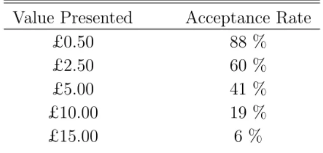
The median value of subjects’ responses was £5. The top five modal values were utilized in the second contingent valuation study, which presented subjects with only one out of the five possible values. Subjects were asked whether they were willing to pay that particular amount to contribute one extra bee-friendly plant to the project. The sample was split between the five values, with 17 subjects responding to the first value of £0.50, 15 subjects responding to the second value of £2.50, 17 subjects responding to the third value of£5.00, 16 subjects responding to the fourth value of £10.00, and 16 subjects responding to the final value of £15.00. The different values presented to respondents and the corresponding acceptance percentages are displayed in Table2. We found that the mean willingness to pay was approximately £4.98.9 This specific value was close enough to the median response in the open-ended question of the first study. Consequently, we rounded the number to the nearest pound, and implemented a conversion rate of 1 plant = £5. Subjects were there-fore presented with choices starting at £50 in the monetary domain and 10 plants in the environmental domain. The plants that were distributed were purchased for£3 to £5 each.
Table 2: Valuation of a Bee-Friendly Plant Value Presented Acceptance Rate
£0.50 88 %
£2.50 60 %
£5.00 41 %
£10.00 19 %
£15.00 6 %
Notes: In the first column, the monetary values that were presented to respondents in the second contingent valuation study are displayed. Subjects were presented withonlyone out of the five possible values. Subjects were asked whether they were willing to pay that particular amount to contribute one extra plant to the project. The sample consisted of 81 subjects who were split between the five values. In the second column, we display the corresponding acceptance percentages; that is, the percentage of subjects who replied that they would be willing to pay that value to contribute one extra plant to the project.
3.3
Tasks
All experimental sessions consisted of six stages with one task in each stage. Subjects were informed of the total number of stages at the start of the experimental session, but 9The mean willingness to pay was estimated using a probit model with the binary response (‘yes’ or ‘no’ to the willingness to pay question) as the dependent variable and the monetary value displayed to the subject as the only explanatory variable along with a constant term.
were introduced to the tasks of the stages as they progressed through the session. The experimental sessions were conducted in the Social Sciences Experimental Lab (SSEL) at the University of Southampton in March and April of 2014. The subjects were recruited from the student population of the University of Southampton using an electronic recruitment system. Subjects were allowed to participate in only one session. A total of 118 students participated in the experiment. The split across gender was almost even: 54% were men and 46% were women. The ages ranged from 18 to 28. The average age was 20 years old. Most subjects (around 60%) were pursuing an economics degree. Students pursuing a mathematics degree (around 12%) had also a large representation in the sample, as well as students pursuing a philosophy degree (around 4%). The remaining 24% of the sample were students studying to earn a degree in one of english, history, modern languages, music, chemistry, law, health sciences and geography. 93% of the subjects were undergraduates; the rest pursued postgraduate studies. Each session had at most 16 subjects (this is the maximum capacity of the lab) and lasted approximately 45 minutes. The minimum number of subjects in a session was 13. The total number of subjects in each subsample and the total number of sessions in each subsample are displayed in the last two rows in Panel B of Table 1. Each participant received £5 as a participation fee. The experimental codes were programmed using the experimental software z-Tree (Fischbacher(2007)). The experimental instructions are provided in the Appendix.
3.3.1 Monetary Discounting (MD) & Environmental Discounting (ED)
The Monetary Discounting (MD) task presented subjects with choices between a smaller sooner amount and a larger later amount. The smaller sooner amount was kept fixed at
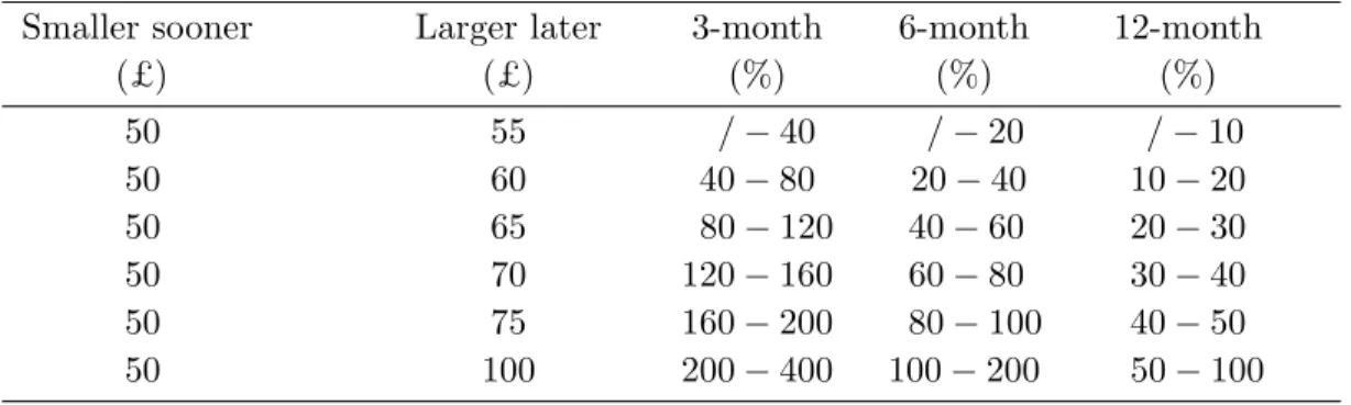
£50, whereas the larger later amount started at £55 and progressively increased to £100 (i.e. £60, £65, £70, £75, £100). Subjects were presented with these six choices for three different delay periods: (i) a 3-month delay period, (ii) a 6-month delay period, and (iii) a 12-month delay period. Thus, in total subjects had to respond to 6×3 = 18 questions. The implied hyperbolic discount-rate brackets in each of the delay periods became progressively smaller. Note that the implied discount-rate brackets were not provided to subjects. In total, we extracted three monetary discount brackets for each subject.10 The binary choices
and the implied hyperbolic discount-rate brackets are displayed in Panel A of Table 3. To calculate the implied discount rates, we used the hyperbolic formula ρ = 12(F/P −1)/T, where ρ is the discount rate, F is the future value, P is the present value and T is the time 10A little less than 92% of subjects had one switching point. Subjects who switched more than once were excluded from the analysis (see Subsection4.1.1).
delay (in months) between the present and the future value (Doyle(2013)).11
Table 3: Binary Choices and Implied Discount-Rate Brackets
Panel A
Monetary Discounting (MD)
Binary Choice Hyperbolic Discount-Rate Brackets Smaller sooner Larger later 3-month 6-month 12-month
(£) (£) (%) (%) (%) 50 55 /−40 /−20 /−10 50 60 40−80 20−40 10−20 50 65 80−120 40−60 20−30 50 70 120−160 60−80 30−40 50 75 160−200 80−100 40−50 50 100 200−400 100−200 50−100 Panel B
Environmental Discounting (ED)
Binary Choice Hyperbolic Discount-Rate Brackets Smaller sooner Larger later 3-month 6-month 12-month
(plants) (plants) (%) (%) (%) 10 11 /−40 /−20 /−10 10 12 40−80 20−40 10−20 10 13 80−120 40−60 20−30 10 14 120−160 60−80 30−40 10 15 160−200 80−100 40−50 10 20 200−400 100−200 50−100
Notes: In Panel A, we display the binary choices and the implied hyperbolic discount-rate brackets in the Monetary Discounting (MD) task. In Panel B, we display the binary choices and the implied hyperbolic discount-rate brackets in the Environmental Discounting (ED) task.
All the intertemporal choices presented to participants incorporated a front-end delay as is standard practice in many such experimental studies. Rather than giving subjects an earlier option that is payable at the end of the experimental session, discounting experiments, typically, make use of a front-end delay where the smaller sooner choice is itself delayed by a short time period (Coller and Williams (1999); Andersen, Harrison, Lau, and Rutstr¨om
(2008)). The main advantage of this approach is that the front-end delay safeguards against possible confounding effects caused by any perceived transaction costs being associated with 11Here, our objective is to investigate subjects’ intertemporal choices across the monetary domain and the environmental domain. We remain agnostic as to the actual numerical value of the discount rate. Calculating the actual discount rate is outside the scope of this study. Nevertheless, our qualitative results are robust to consistent changes in the functional form across the two domains.
the larger later payment (Harrison and Lau (2005)).
The payment method was designed to further reduce any perceived transaction costs. Subjects were given a requisition form at the end of the experimental session, which detailed their payoffs. The requisition form had to be dropped off at the Finance Office (in the School of Social Sciences at the University of Southampton) and participants were paid by direct debit by the Finance Office on the date specified on the form. The precise process was explained in the experimental instructions.
In the Environmental Discounting (ED) task, subjects were presented with the same setup as in the MD task; that is, six binary choices were displayed for each of the (three) different delay periods. Analogous to the task above, three environmental discount brackets were obtained for each subject. The only difference between this task and the previous one is that subjects were presented with the environmental instrument (i.e. plants) instead of money. The binary choices presented to subjects and the implied hyperbolic discount-rate brackets are displayed in Panel B of Table3.
3.3.2 Monetary Risk Aversion Test (MRAT) & Environmental Risk Aversion Test (ERAT)
The two tests served to elicit subjects’ risk aversion in the monetary domain and the en-vironmental domain. We used a variant of the Eckel-Grossman test (Eckel and Grossman
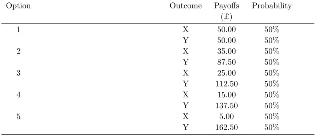
(2002); Eckel and Grossman (2008)), where subjects were presented with five gambles of varying riskiness and were required to select the one they prefer. All gambles had two possi-ble outcomes: Outcome X with 50% likelihood and Outcome Y with 50% likelihood; that is, both outcomes were equiprobable. In addition, the expected payoffs were easy to calculate and the increasing variance as the gambles got riskier was significantly large to be noticeable. This test is a simplified version of the one designed by Holt and Laury (2002), albeit still elicits sufficient heterogeneity in subjects’ responses (Eckel and Grossman (2008)).
The Monetary Risk Aversion Test (MRAT) was set at a magnitude level that was com-parable to the choices given to subjects in the discounting tasks. The gambles started at an option with identical outcomes (i.e. a gain of £50) and moved to options of increasing variance at the point where the last option’s equiprobable outcomes were £5 and £162.50. Expected payoffs increased as you moved down the table, so choices further down indicated lowerrisk aversion. The Environmental Risk Aversion Test (ERAT) was matched in magni-tude to the MRAT at the same conversion rate of money per plant (£5 per plant) used in the discounting tasks. Analogous to the MRAT, the first option had identical outcomes, whereas the last option’s equiprobable outcomes were 1 plant and 33 plants. The lists of gambles
Table 4: Risk Aversion Tests
Panel A
Monetary Risk Aversion Test (MRAT)
Option Outcome Payoffs Probability
(£) 1 X 50.00 50% Y 50.00 50% 2 X 35.00 50% Y 87.50 50% 3 X 25.00 50% Y 112.50 50% 4 X 15.00 50% Y 137.50 50% 5 X 5.00 50% Y 162.50 50% Panel B
Environmental Risk Aversion Test (ERAT)
Option Outcome Payoffs Probability
(plants) 1 X 10 plants 50% Y 10 plants 50% 2 X 7 plants 50% Y 18 plants 50% 3 X 5 plants 50% Y 23 plants 50% 4 X 3 plants 50% Y 28 plants 50% 5 X 1 plant 50% Y 33 plants 50%
Notes: Panel A displays the Monetary Risk Aversion Test (MRAT). Panel B displays the Environmental Risk Aversion Test (ERAT). Both panels follow the same structure. In the first column, the 5 options available to subjects are listed. In the second column, the possible outcomes of each option are listed: Outcome X or Outcome Y. In the third column, the payoffs associated with each outcome in each option are listed. Note that the inability to express decimals in plants led us to the rounding up of payoffs in this domain. In column four, the probability of that specific outcome occurring is listed.
presented in the MRAT and the ERAT are displayed in Panel A and Panel B, respectively, in Table 4.
3.3.3 Cognitive Reflection Test (CRT) & Questionnaire (Q)
The Cognitive Reflection Test (CRT) was proposed byFrederick(2005) as a way of measuring a specific type of cognitive ability−that of suppressing a spontaneous response in favor of a more deliberately-thought-out one. The CRT consists of 3 questions. In order to successfully complete the CRT subjects were required to question their initial response and devote some cognitive power to realize that it was incorrect and, consequently, arrive at the correct answer. The inclusion of the CRT task allows us to capture the heterogeneity in subjects’ reflective ability. More specifically, cognitive ability could plausibly be increasingly relevant to the evaluation of intertemporal (monetary and environmental) choices and (monetary and environmental) risk aversion. The three CRT questions are included in the Appendix.
Finally, in the last stage, we administered the Questionnaire (Q). The questionnaire consisted of questions of socio-demographic nature as well as 17 questions taken from the Segmentation Model developed by DEFRA (2008).12 The latter part pertained to subjects’ values, attitudes and motivations as well as current behaviors and barriers to change. In addition, the questions covered topics, such as climate change, recycling, transportation and water use. The Q was administered in the last stage in order to remove any unintentional impact these questions might have on the environmental intertemporal choices and environ-mental risk aversion of subjects.
3.4
Payment Mechanism
The experimental design applied a variant of the random-lottery incentive scheme, where subjects make a number of decisions knowing that, at the end of the experimental session, one of these decisions will be selected for payment. There is a vast literature testing the va-lidity of this payment scheme. Laury(2012) found that subjects do not scale down decisions when they are only being paid for a subset of these decisions. Along the same lines,Cubitt, Starmer, and Sugden(1998) confirmed that such design does not contaminate elicited prefer-ences. Hey and Lee (2005) showed that subjects separate the various questions, and respond to each question individually and in isolation from the rest; thus, incentives are retained. A 12The model segments the population into seven behavioral groups using a number of questions on envi-ronmental attitudes and the respondents’ age. DEFRA has developed this model in order to further advance behavioral change through social marketing strategies that target specific segments of the population. Their objective is to achieve a more environmentally-friendly lifestyle for the public. Segmentation models are a popular way of investigating the behavior of individuals as it pertains to specific functions of their everyday life, such as transportation choices and water consumption. The advantage of the DEFRA model is that it targets attitudes towards many different environmental sectors, thus achieving a classification that captures an individual’s overall attitude to issues of an environmental nature (Jesson(2009);Barr, Shaw, and Coles
value-added of this approach is that it neutralizes the income effect that would otherwise be experienced as subjects progress through the periods. Our approach was to apply a double layered random-lottery incentive payment scheme. More specifically, two subjects in each experimental session were randomly selected to be paid for their choices. The first subject selected was paid for either the choice made in the MD task or the choice made in the ED task, where each task had an equal probability of being selected. Once the domain was selected, one of the 18 questions was drawn and the subject’s choice in that question was paid (with money or plants accordingly). The second subject selected was paid for either the choice made in the MRAT or the choice made in the ERAT, where each test had an equal probability of being selected. Once the test was selected, an outcome was drawn (X or Y where each outcome had an equal probability of being selected) and the subject was paid (with money or plants accordingly) based on the gamble chosen.
The random selection was carried out using a bingo machine that was prominently dis-played in the lab. Bingo balls were placed on subjects’ desks with the terminal ID number on the ball. Subjects placed the balls into the bingo machine themselves at the end of the experimental session and witnessed the random selection. This was necessary to ensure com-plete transparency of the process. However, the choices of the subjects selected were not revealed to the other subjects as that would violate the confidentiality with respect to their earnings.
3.5
General Hypotheses
Our objective in this study is to investigate subjects’ intertemporal choices and risk aversion across the monetary domain and the environmental domain. Based on the existing literature (Hardisty and Weber (2009)), we hypothesized that the domain has no impact on subjects’ intertemporal choices − referred to as domain independence (Chapman (2003)). This hy-pothesis is tested by comparing the intertemporal choices taken in the monetary domain with those taken in the environmental domain. The first general hypothesis is thus formulated as follows.
H1 (Domain Independence in Time Preferences): Subjects’ discounting behavior is the same across the monetary and the environmental domains.
In an analogous manner, we hypothesized that subjects’ risk aversion is independent of the domain. The second hypothesis is stated as follows.
H2 (Domain Independence in Risk Aversion): Subjects’ risk aversion is the same across the monetary and the environmental domains.
4
Results
The six hypotheses on the effect of domain are formally tested next. Each hypothesis is matched with the corresponding result; that is, result i is a report on the test of hypothesis i.
4.1
Descriptive Statistics
4.1.1 Time Preferences
Recall that subjects had to decide on the switching point in the 3-month delay period, the 6-month delay period, the 12-6-month delay period for both the monetary and the environmental domains. Subjects that switched twice within the same time-delay period were taken out of the data analysis. Thus, 10 subjects were excluded from the sample leaving us with a total of 108 observations.
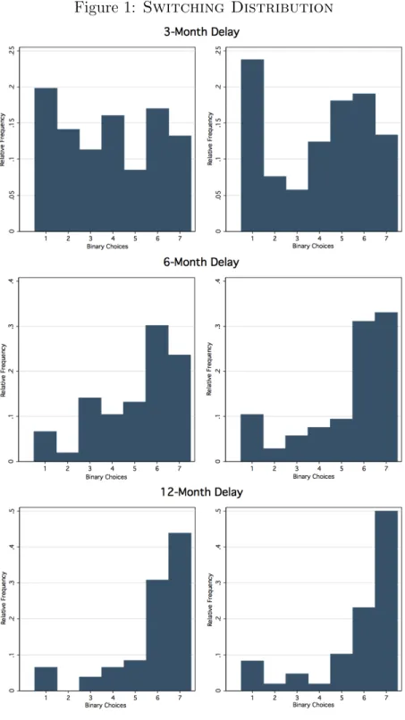
We present next the switching distribution of subjects in the three delay periods in the monetary domain and in the three delay periods in the environmental domain. This information is displayed in Figure1. An individual with a binary choice of 1 in the monetary domain, chose the larger later amount of £55 in lieu of the earlier smaller amount of £50, and an individual with a binary choice of 1 in the environmental domain, chose the larger later amount of 11 plants in lieu of the earlier smaller amount of 10 plants. An individual with a binary choice of 7 in either the monetary or the environmental domain, always chose the earlier smaller amount. The mean switch in the 3-month delay period (MD 3.8/ED 4.0) implies an annual discount-rate bracket between 80% and 160%. The mean switch in the 6-month delay period (MD 5.1/ED 5.3) implies an average discount-rate bracket between 80% and 200%. Finally, the mean switch in the 12-month delay period (MD 5.5/ED 5.7) implies an average discount-rate bracket between 40% and 100%.
We next allocate subjects into three categories based on their discounting behavior in the monetary domain and the environmental domain while controlling for the time delay. More specifically, we provide the frequency and percentage of subjects that exhibited one of the three discounting patterns: (i) constant discounting across domains, (ii) higher discounting in the environmental domain, and (iii) lower discounting in the environmental domain. The findings are displayed in Table5. Over the three time-delay periods, on average, the number of subjects that exhibited a constant discounting behavior across the two domains was 30%, 40% of the subjects exhibited a higher discount rate in the environmental domain, and 30% of the subjects exhibited a lower discount rate in the environmental domain.
Figure 1: Switching Distribution
Notes: We display, on the left, the relative frequency of subjects’ switching distributions across the discount-ing tasks in the monetary domain, and we display, on the right, the relative frequency of subjects’ switchdiscount-ing distributions across the discounting tasks in the environmental domain. An individual with a binary choice of 1 in the monetary domain, chose the larger later amount of£55 in lieu of the earlier smaller amount of £50, and an individual with a binary choice of 1 in the environmental domain, chose the larger later amount of 11 plants in lieu of the earlier smaller amount of 10 plants. An individual with a binary choice of 7 in either the monetary or the environmental domain, always chose the earlier smaller amount.
Table 5: Discounting Patterns Across Domains
Time Delay: 3-month 6-month 12-month
Freq. % Freq. % Freq. %
Constant discounting across domains 27 25 29 27 42 39 Higher environmental discounting 46 43 48 44 35 32
Lower environmental discounting 35 32 31 29 31 29
Total 108 108 108
Notes: We display information on subjects’ discounting behavior in the monetary domain and the environ-mental domain while controlling for the time delay.
4.1.2 Risk Aversion
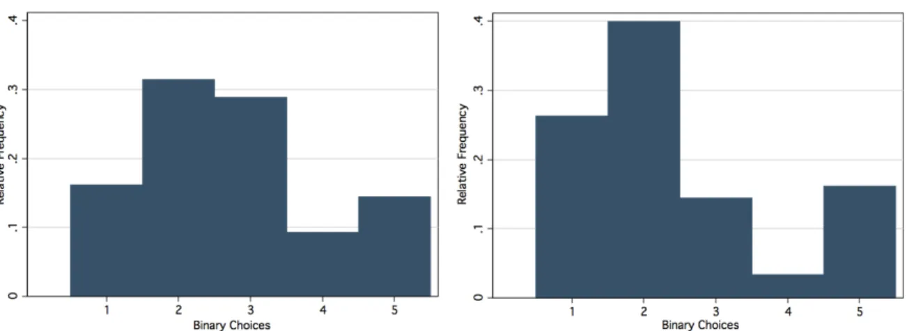
In the tests on risk aversion, subjects were given five gambles to choose from, where each gamble featured two possible outcomes: Outcome X with 50% likelihood and Outcome Y with 50% likelihood. The gambles started at a non-degenerate gamble and moved to degenerate gambles of increasing variance and expected payoffs. In the Monetary Risk Aversion Test (MRAT), 18% of subjects chose the non-degenerate gamble, 59% of subjects chose one of the next two gambles, while the remaining 23% chose one of the last two gambles. In the Environmental Risk Aversion Test (ERAT), 28% of subjects chose the non-degenerate gamble, 54% of subjects chose one of the next two gambles, and the remaining 18% chose one of the last two gambles. The relative frequency of subjects’ gambles across the MRAT and ERAT is displayed in Figure2.
Figure 2: Distribution of Risk Aversion
Notes: We display, on the left, the relative frequency of subjects’ gambles across the MRAT, and we display, on the right, the relative frequency of subjects’ gambles across the ERAT. Binary choices indicate the gambles chosen by the subjects.
4.1.3 Cognitive Reflection Test & Questionnaire
The Cognitive Reflection Test (CRT) aims to measure subjects’ reflective ability. The test requires subjects to answer three questions, where each question has 4 possible answers. The CRT score consists of one positive point for every correct answer given. The score therefore ranges from 0 to 3. 34% of the subjects answered all three questions correctly, while 18% of subjects got all three questions wrong. The spread of scores suggests a dispersion of reflective ability amongst subjects. The distribution for the CRT is shown in Figure 3.
Figure 3: Distribution of CRT Scores
0 0 0 .1 .1 .1 .2 .2 .2 .3 .3 .3 Relative Frequency Re la ti ve F re qu en cy Relative Frequency 0 0 0 1 1 1 2 2 2 3 3 3 Score Score Score
Notes: We report the relative frequency of subjects’ CRT scores. The CRT score consists of one positive point for every correct answer given.
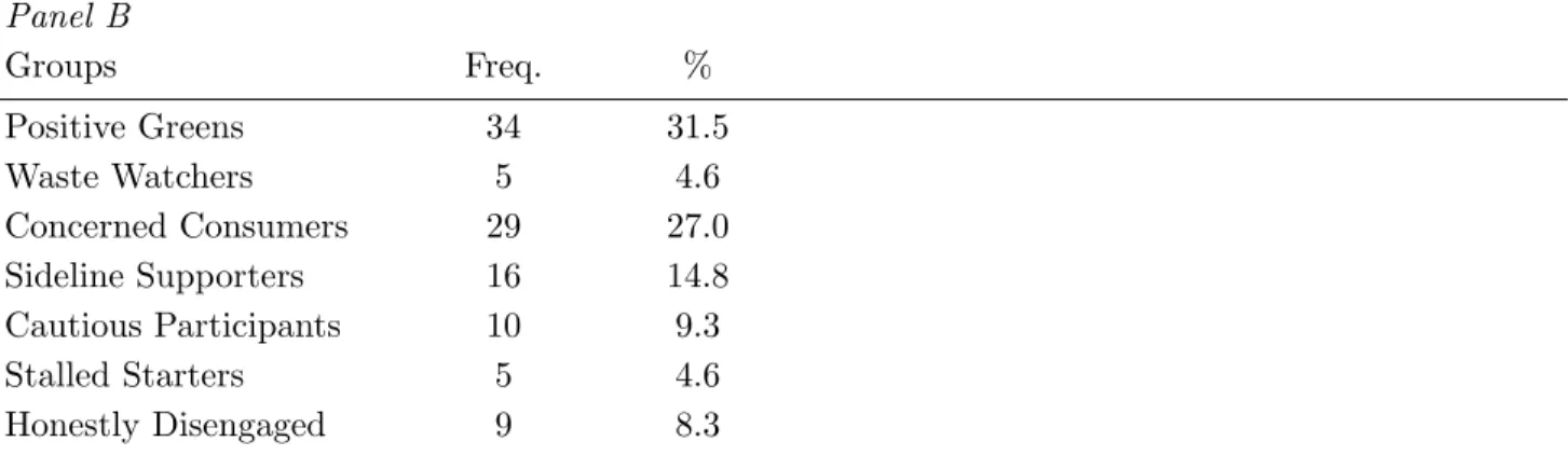
The questionnaire consisted of questions of socio-demographic nature as well as 17 ques-tions taken from the Segmentation Model developed byDEFRA(2008). The questions from the Segmentation Model are provided in Panel A of Table 6. The model segments the re-spondents into 7 behavioral groups. The frequencies and corresponding percentages of the seven groups are displayed in Panel B of Table 6. The first four groups are considered pro-environmental. In our sample, almost 78% of the respondents belong to one of the top four pro-environmental groups. We further classify subjects that belong to the top four groups as exhibiting environmental awareness.
Table 6: Segmentation Model
Panel A
Questions
I would only travel by bus if I had no other choice.
For the sake of the environment, car users should pay higher taxes.
People who fly should bear the cost of the environmental damage that air travel causes. I don’t pay much attention to the amount of water I use.
People have a duty to recycle.
We are close to the limit of the number of people that earth can support. The earth has very limited room and resources.
If things continue on their current course, we will soon experience a major environmental disaster. The so-called ‘environmental crisis’ facing humanity has been greatly exaggerated.
It would embarrass me if my friends thought my lifestyle was purposefully environmentally friendly. Being green is an alternative lifestyle, it’s not for the majority.
I find it hard to change my habits to be more environmentally friendly. It’s only worth doing environmentally-friendly things if they save you money. The effects of climate change are too far in the future to really worry me.
It’s not worth me doing things to help the environment if others don’t do the same.
It’s not worth Britain trying to combat climate change, other countries will just cancel what we do. Which of these best describes how you feel about your current lifestyle and the environment?
Panel B Groups Freq. % Positive Greens 34 31.5 Waste Watchers 5 4.6 Concerned Consumers 29 27.0 Sideline Supporters 16 14.8 Cautious Participants 10 9.3 Stalled Starters 5 4.6 Honestly Disengaged 9 8.3
Notes: Panel A displays the questions that constitute the Segmentation Model, and Panel B classifies the 108 respondents into 7 behavioral groups (DEFRA (2008)). With the exception of the last question, the possible responses to all other statements were: ‘Strongly agree,’ ‘Tend to agree,’ ‘Neither agree nor disagree,’ ‘Strongly disagree,’ and ‘Don’t know.’ In the last question, the possible responses were: ‘I’d like to do a lot more to help the environment,’ ‘I’d like to do a bit more to help the environment,’ ‘I’m happy with what I do at the moment,’ and ‘Don’t know.’
4.2
Order Effects
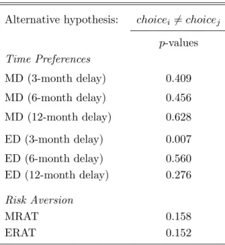
The principal drawback of a ‘within-subject’ experimental design is the possibility that the order in which the subjects are presented with the tasks might influence their choices. Recall that in our setup, we allowed for four subsamples (see Table 1). In Table 7, we test for differences in subjects’ choices across the four subsamples. More specifically, we use pairwise χ2-tests, where theH0 states that subjects’ choice in a specific task across subsamples is not
statistically different. Thus, rejecting the null would imply that the setup is confounded with order effects. With the exception of the 3-month delay in the environmental discounting task, our design does not seem to be susceptible to order effects. However, given the possibility of an order bias, we imposed a consistency check to our data analysis. Specifically, the same analysis was carried out using a much restricted dataset that consisted of data from only the first task of the subsamples. The two main results reported in the next two subsections withstandthe consistency check imposed.
Table 7: Order Effects
Alternative hypothesis: choicei 6=choicej
p-values Time Preferences MD (3-month delay) 0.409 MD (6-month delay) 0.456 MD (12-month delay) 0.628 ED (3-month delay) 0.007 ED (6-month delay) 0.560 ED (12-month delay) 0.276 Risk Aversion MRAT 0.158 ERAT 0.152
Notes: We utilize the χ2-test to determine whether subjects’ choice in a specific task differs (i6=j) across subsamples.
4.3
Domain Differences in Time Preferences & Risk Aversion
The first hypothesis aims to determine whether a change in domain has an effect on subjects’ discounting behavior. We formally test our hypothesis using a standard χ2-test, where the
H0 states that the discounting behavor across the monetary and the environmental domains
is similar when controlling for the time delay. The results are displayed in Table 8. Similar to the findings of Hardisty and Weber (2009), we find that we cannot reject the H0. This
finding is formalized next in our first main result.13
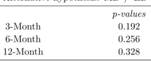
RESULT 1: Subjects’ discounting behavior is the same across the monetary and the envi-ronmental domains.
Support. The χ2-test conducted does not find any significant differences in discounting across the monetary domain and the environmental domain.
Table 8: χ2-Tests on Domain Differences in Time Preferences
Alternative hypothesis: MD 6= ED
p-values
3-Month 0.192
6-Month 0.256
12-Month 0.328
Notes: We reportp-values from the χ2-test, where theH0 states that the discounting behavior across the monetary and the environmental domains is similar when controlling for the time delay.
The second hypothesis aims to determine whether a change in domain has an impact on subjects’ risk aversion. Analogous to the analysis in the previous subsection, we, also, run a standard χ2-test to examine whether subjects’ choices on gambles are the same across domains. Table9shows the result of the test. TheH0 is rejected at the 1% level of statistical
significance; that is, there exists serious evidence of a domain effect in subjects’ choices on gambles.
We, also, run two ordered probit regressions in Table10with subjects’ choices in the tests on risk aversion as the categorical dependent variable. Domain is an explanatory dummy regression variable, which takes the value of 1 if the risk aversion has been obtained from the ERAT and 0 if the risk aversion has been obtained from the MRAT. We investigate two 13Recall that the experimental data on the repeated binary intertemporal choices are transformed into a single switching point; the latter produces a discount-rate interval, which contains the indifference point of each subject. Given that the data is of an interval nature and this feature is not captured by the above test, we, also, run an interval regression, which allows for the specification of the (discount-rate) brackets presented to participants as the dependent variable. More specifically, it allows for the first and last brackets to be open; therefore, the first bracket has no minimum value and the last bracket has no maximum value. The interval regression is run on the log of the discount rates with domain as an explanatory dummy variable, which takes the value of 1 for discounting in the environmental domain and 0 otherwise. The latter model confirms the aforementioned main result.
Table 9: χ2-Test on Domain Differences in Risk Aversion
Alternative hypothesis: MRAT6= ERAT
p-value 0.001
Notes: We utilize theχ2-test to determine whether subjects’ choices on gambles are the same across the two domains.
specifications: Model 1 and Model 2. Model 2 builds upon the first model by adding the gender variable, an interaction variable between gender and domain, a variable on whether the subject’s parents own their home, a variable on whether the subject belongs in one of the top four, pro-environmental groups of DEFRA (2008) (i.e. exhibits environmental awareness), and a variable on whether the subject scored at least 2 questions correctly on the CRT. Crucially, we find that subjects exhibit a higher degree of risk aversion in the environmental domain relative to the monetary domain.14 These findings culminate in our
second main result.
RESULT 2: Subjects’ risk aversion is statistically different across the monetary and the environmental domains. Specifically, subjects exhibit higher levels of risk aversion in the environmental domain.
Support. The results of theχ2-test and the ordered probit regressions indicate significant differences in subjects’ risk aversion across the two domains.
In Model 2, we observe that the domain and gender regressors are both significant, while the interaction regressor (domain× gender) is not. This implies that both men and women exhibit higher levels of risk aversion in the environmental domain than in the monetary one, and that women exhibit higher levels of risk aversion than men in both the monetary and the environmental domains. The finding that women are more risk averse than men in the monetary domain corroborates existing results due toEckel and Grossman(2002). Crucially, we show this finding to, also, hold in the environmental domain.
14A negative coefficient indicates an increase in the likelihood that a subject will choose one of the earlier (safer) gambles, thereby displaying a higher degree of risk aversion.
Table 10: Ordered Probit Results for Domain Differences in Risk Aversion
Variables Model 1 Model 2
Domain -0.296*** -0.302* (0.110) (0.166) Gender -0.615*** (0.214) Domain ×Gender 0.098 (0.242) Own home -0.178 (0.255) Environmental awareness -0.032 (0.192) High CRT -0.112 (0.192) Order 1 -0.129 -0.066 (0.243) (0.293) Order 2 -0.348 -0.358 (0.214) (0.231) Order 3 0.022 -0.035 (0.252) (0.256)
Notes: A subject’s choice is the categorical dependent variable. The two models vary in the number of explanatory variables included. ‘Domain’ is a dummy that takes the value of 1 in the environmental domain and 0 in the monetary domain, ‘Gender’ is a dummy that takes the value of 1 if the subject is female and 0 otherwise, ‘Domain×Gender’ is an interaction variable for the previous two dummies, ‘Own home’ is a dummy that takes the value of 1 if the subject’s parents own their home and 0 otherwise, ‘Environmental awareness’ is a dummy that takes the value of 1 if the subject belongs in one of the top four, pro-environmental groups ofDEFRA(2008) and 0 otherwise, and ‘High CRT’ is a dummy that takes the value of 1 if the subject scored at least 2 questions correctly on the CRT and 0 otherwise. The three ‘Order’ variables are dummies that account for the four possible orders that the tasks could have been undertaken. All standard errors are reported in parentheses. * Significant at the 10% level ** Significant at the 5% level *** Significant at the 1% level.
4.4
Cognitive Ability & Environmental Awareness
The Cognitive Reflection Test (CRT) and the questionnaire enabled us to obtain both a measure of subjects’ cognitive ability as well as insights to subjects’ environmental awareness, which could possibly relate to the way different domains were evaluated by subjects. Recall that a subject exhibits environmental awareness if he/she has been classified in one of the top four, pro-environmental groups in Panel B of Table6. We investigate next whether subjects’
cognitive ability and environmental awareness correlate with individual time preferences and risk aversion in the two domains. We find that neither time preferences nor risk aversion is correlated with CRT or environmental awareness across the two domains.15
We apply next a multinomial probit regression on the distinct discounting patterns iden-tified in Subsection 4.1.1 in order to identify any variable(s) that might correlate with a subject’s discounting pattern. Our findings are displayed in Table 11. As a base, we used the subjects that exhibited a constant discounting behavior across the two domains. We find that parental ownership of the home is a significant factor, which correlates negatively with both subjects exhibiting a higher discounting in the environmental domain and those exhibiting a lower discounting in the environmental domain. Consequently, subjects hav-ing parents that owned their own home correlates positively with subjects that exhibit a constant discounting pattern across the two domains. In addition, we find a significant cor-relation between subjects exhibiting environmental awareness and lower discounting in the environmental domain relative to the monetary domain.
5
Concluding Remarks
We study experimentally subjects’ time preferences and risk aversion across two domains: the monetary domain and the environmental domain. Our study is the first to utilize an in-centivized experimental design: in the monetary domain, time preferences and risk aversion are elicited with real monetary payoffs, whereas in the environmental domain, time pref-erences and risk aversion are elicited using real, bee-friendly plants. Contrasting subjects’ intertemporal choices across the monetary and environmental domains, we find that subjects’ discounting behavior is not statistically different (RESULT 1). In sharp contrast, subjects’ risk aversion is significantly different across the monetary domain and the environmental domain; specifically, subjects tend to be unwilling to take on large gambles when it comes to bee-friendly plants (RESULT 2). This result is not gender-specific; that is, both men and women exhibit a higher degree of risk aversion in the environmental domain relative to the monetary domain. Finally, we find that women are more risk averse than men in both the monetary and the environmental domains.
Ideally, these results would have to be evaluated across two important dimensions. First, time preferences and risk aversion in the environmental domain should be tested with other 15This is a departure from the findings ofFrederick(2005). We conjecture that differences in the experi-mental design (Frederick’s design was not incentivized) can account for the divergence.
Table 11: Determinants of Discounting Pattern
Variables Higher environmental Lower environmental discounting discounting Age 0.212 0.289 (0.175) (0.185) Gender 0.517 0.758 (0.548) (0.580) Expenditure 0.002 -0.001 (0.002) (0.002) Own home -2.015** -2.358** (0.789) (0.962) Environmental awareness 0.695 1.390** (0.552) (0.675) High CRT 0.033 -0.320 (0.258) (0.275) Constant -6.930* -8.483** (3.321) (3.556)
Notes: We report the coefficients from the multinomial probit regression conducted. As a base, we used the subjects that exhibited a constant discounting behavior across the two domains. The variable ‘Age’ corresponds to the age of the participant, the variable ‘Gender’ is a dummy that takes the value of 1 if the subject is female and 0 otherwise, the variable ‘Expenditure’ is a self-reported assessment of the money the subject spends each month on expenses other than accommodation, the variable ‘Own home’ is a dummy that takes the value of 1 if the subject’s parents own their home and 0 otherwise, ‘Environmental awareness’ is a dummy that takes the value of 1 if the subject belongs in one of the top four, pro-environmental groups ofDEFRA(2008) and 0 otherwise, and the variable ‘High CRT’ is a dummy that takes the value of 1 if the subject scored at least 2 questions correctly on the CRT and 0 otherwise. All standard errors are reported in parentheses. * Significant at the 10% level ** Significant at the 5% level *** Significant at the 1% level
environmental instruments and compared to time preferences and risk aversion in the mon-etary domain to determine the robustness of the aforementioned findings. For instance, it would be interesting to include instruments that are closer to resembling private goods, such as energy-saving light bulbs or even instruments that confer little private benefit to the recipient, such as supporting endangered species. Second, time preferences and risk aver-sion should be tested across a much broader array of domains to identify domain-specificity where such exists. The current research highlights that a direct mapping of results from the monetary domain to the environmental domain is risky. We believe the same holds true for other domains.
Acknowledgements
We are grateful to Daniel Read for helpful discussion of this paper. We are, also, thankful to the Department for Environment, Food & Rural Affairs for providing the questionnaire and guidance to the methodology to segment the respondents into the 7 behavioral groups. The research was supported by research funds from the Economic and Social Research Coun-cil (ESRC) and the Strategic Research Development Fund (SRDF) of the University of Southampton.
References
Andersen, Steffen, Glenn W. Harrison, Morten I. Lau, and E. Elisabet Rutstr¨om. “Eliciting Risk and Time Preferences.” Econometrica 76, 3: (2008) 583–618.
Barr, Stewart, Gareth Shaw, and Tim Coles. “Sustainable Lifestyles: Sites, Practices, and Policy.” Environment and Planning A43, 12: (2011) 3011–29.
B¨ohm, Gisela, and Hans-R¨udiger Pfister. “Consequences, Morality, and Time in Environ-mental Risk Evaluation.” Journal of Risk Research 8, 6: (2005) 461–79.
Cairns, John, and Marjon van der Pol. “Do People Value Their Own Future Health Differ-ently From Others’ Future Health?” Medical Decision Making 19, 4: (1999) 466–72. Cairns, John A. “Health, Wealth and Time Preference.” Project Appraisal 7, 1: (1992)
31–40.
Camerer, Colin F., and Robin M. Hogarth. “The Effects of Financial Incentives in Ex-periments: A Review and Capital-Labor-Production Framework.” Journal of Risk and Uncertainty 19, 1-3: (1999) 7–42.
Chapman, Gretchen B. “Temporal Discounting and Utility for Health and Money.” Journal of Experimental Psychology Learning Memory and Cognition 22, 3: (1996) 771–91.
. “Time Discounting of Health Outcomes.” In Time and Decision: Economic and Psychological Perspectives on Intertemporal Choice, edited by George Loewenstein, Daniel Read, and Roy F. Baumeister, Russell Sage Foundation, 2003.
Chapman, Gretchen B., and Arthur S. Elstein. “Valuing the Future: Temporal Discounting of Health and Money.” Medical Decision Making 15, 4: (1995) 373–86.
Charness, Gary, Uri Gneezy, and Michael A. Kuhn. “Experimental Methods: Between-Subject and Within-Between-Subject Design.” Journal of Economic Behavior and Organization 81, 1: (2012) 1–8.
Coller, Maribeth, and Melonie B. Williams. “Eliciting Individual Discount Rates.” Experi-mental Economics 2, 2: (1999) 107–27.
Cubitt, Robin P., Chris Starmer, and Robert Sugden. “On the Validity of the Random Lottery Incentive System.” Experimental Economics 1, 2: (1998) 115–31.
Cummings, Ronald G., Glenn W. Harrison, and E. Elisabet Rutstr¨om. “Homegrown Values and Hypothetical Surveys: Is the Dichotomous Choice Approach Incentive-Compatible?” The American Economic Review 85, 1: (1995) 260–6.
DEFRA. “A Framework for Pro-Environmental Behaviours.” Technical report, Department for Environment Food and Rural Affairs, 2008.
Dohmen, Thomas, Armin Falk, David Huffman, Uwe Sunde, J¨urgen Schupp, and Gert G. Wagner. “Individual Risk Attitudes: Measurement, Determinants, and Behavioral Con-sequences.” Journal of the European Economic Association 9, 3: (2011) 522–50.
Doyle, John R. “Survey of Time Preference, Delay Discounting Models.” Judgment and Decision Making 8, 2: (2013) 116–35.
Eckel, Catherine C., and Philip J. Grossman. “Sex Differences and Statistical Stereotyping in Attitudes Toward Financial Risk.” Evolution and Human Behavior 23, 4: (2002) 281–95.
. “Forecasting Risk Attitudes: An Experimental Study Using Actual and Forecast Gamble Choices.” Journal of Economic Behavior and Organization 68, 1: (2008) 1–17. Fischbacher, Urs. “z-Tree: Zurich Toolbox for Ready-Made Economic Experiments.”
Exper-imental Economics 10, 2: (2007) 171–8.
Frederick, Shane. “Cognitive Reflection and Decision Making.” The Journal of Economic Perspectives 19, 4: (2005) 25–42.
Frederick, Shane, George Loewenstein, and Ted O’Donoghue. “Time Discounting and Time Preference: A Critical Review.” Journal of Economic Literature 40, 2: (2002) 351–401. Gattig, Alexander, and Laurie Hendrickx. “Judgmental Discounting and Environmental
Risk Perception: Dimensional Similarities, Domain Differences, and Implications for Sus-tainability.” Journal of Social Issues 63, 1: (2007) 21–39.
Green, Leonard, Astrid F. Fry, and Joel Myerson. “Discounting of Delayed Rewards: A Life-Span Comparison.” Psychological Science 5, 1: (1994) 33–6.
Hardisty, David J., Katherine F. Thompson, David H. Krantz, and Elke U. Weber. “How to Measure Time Preferences: An Experimental Comparison of Three Methods.” Judgment and Decision Making 8, 3: (2013) 236–49.
Hardisty, David J., and Elke U. Weber. “Discounting Future Green: Money Versus the Environment.” Journal of Experimental Psychology: General 138, 3: (2009) 329–40.
Harrison, Glenn W., and Morten I. Lau. “Is the Evidence for Hyperbolic Discounting in Humans Just an Experimental Artefact?” Behavioral and Brain Sciences 28: (2005) 657–7.
Hey, John D., and Jinkwon Lee. “Do Subjects Separate (or Are They Sophisticated)?” Experimental Economics 8, 3: (2005) 233–65.
Holt, Charles A., and Susan K. Laury. “Risk Aversion and Incentive Effects.” The American Economic Review 92, 5: (2002) 1644–55.
Jesson, Jill. “Household Waste Recycling Behavior: A Market Segmentation Model.” Social Marketing Quarterly 15, 2: (2009) 25–38.
Kirby, Kris N., and Nino N. Marakovi. “Modeling Myopic Decisions: Evidence for Hyperbolic Delay-Discounting within Subjects and Amounts.” Organizational Behavior and Human Decision Processes 64, 1: (1995) 22–30.
Kroll, Yoram, Haim Levy, and Amnon Rapoport. “Experimental Tests of the Separation Theorem and the Capital Asset Pricing Model.” The American Economic Review 78, 3: (1988) 500–19.
Laury, Susan K. “Pay One or Pay All: Random Selection of One Choice for Payment.” Discussion Paper, Andrew Young School, Georgia State University .
Madden, Gregory J., Warren K. Bickel, and Eric A. Jacobs. “Discounting of Delayed Rewards in Opioid-Dependent Outpatients: Exponential or Hyperbolic Discounting Functions?” Experimental and Clinical Psychopharmacology 7, 3: (1999) 284–93.
Nordhaus, William D. “A Review of the “Stern Review on the Economics of Climate Change”.” Journal of Economic Literature 45, 3: (2007) 686–702.
Raineri, Andres, and Howard Rachlin. “The Effect of Temporal Constraints on the Value of Money and Other Commodities.” Journal of Behavioral Decision Making 6, 2: (1993) 77–94.
Read, Daniel, Shane Frederick, Burcu Orsel, and Juwaria Rahman. “Four Score and Seven Years from Now: The Date/Delay Effect in Temporal Discounting.” Management Science 51, 9: (2005) 1326–35.
Riddel, Mary. “Comparing Risk Preferences over Financial and Environmental Lotteries.” Journal of Risk and Uncertainty 45, 2: (2012) 135–57.
Stern, Nicholas. “The Economics of Climate Change: The Stern Review.” Technical report, Cambridge University Press, 2007.
Viscusi, W. Kip, Joel Huber, and Jason Bell. “Estimating Discount Rates for Environmental Quality from Utility-Based Choice Experiments.”Journal of Risk and Uncertainty 37, 2-3: (2008) 199–220.
Weber, Elke U., Ann-Ren´ee Blais, and Nancy E. Betz. “A Domain-Specific Risk-Attitude Scale: Measuring Risk Perceptions and Risk Behaviors.” Journal of Behavioral Decision Making 15, 4: (2002) 263–90.
Weitzman, Martin L. “A Review of The Stern Review on the Economics of Climate Change.” Journal of Economic Literature 45, 3: (2007) 703–24.