Quadratic functional estimation in view of minimax
goodness-of-fit testing from noisy data
Cristina Butucea
To cite this version:
Cristina Butucea. Quadratic functional estimation in view of minimax goodness-of-fit testing from noisy data. 2004. <hal-00002985>
HAL Id: hal-00002985
https://hal.archives-ouvertes.fr/hal-00002985
Submitted on 30 Sep 2004
HAL is a multi-disciplinary open access archive for the deposit and dissemination of sci-entific research documents, whether they are pub-lished or not. The documents may come from teaching and research institutions in France or abroad, or from public or private research centers.
L’archive ouverte pluridisciplinaire HAL, est destin´ee au d´epˆot et `a la diffusion de documents scientifiques de niveau recherche, publi´es ou non, ´emanant des ´etablissements d’enseignement et de recherche fran¸cais ou ´etrangers, des laboratoires publics ou priv´es.
Universit´
es de Paris 6 & Paris 7 - CNRS (UMR 7599)
PR´
EPUBLICATIONS DU LABORATOIRE
DE PROBABILIT´
ES & MOD`
ELES AL´
EATOIRES
Quadratic functional estimation in view of minimax goodness-of-fit testing
from noisy data C. BUTUCEA
SEPTEMBRE 2004
Pr´epublication no 936
Laboratoire de Probabilit´es et Mod`eles Al´eatoires, CNRS-UMR 7599, Universit´e Paris VI & Universit´e Paris VII,
4, place Jussieu, Case 188, F-75252 Paris Cedex 05. &
Quadratic functional estimation in view of
minimax goodness-of-fit testing from noisy data
Cristina Butucea
1Laboratoire de Probabilit´es et Mod`eles Al´eatoires (UMR CNRS 7599),
Univer-sit´e Paris VI, 4, pl.Jussieu, Boˆıte courrier 188, 75252 Paris, France
2Modal’X, Universit´e Paris X, 200, avenue de la R´epublique 92001 Nanterre Cedex,
France, e-mail: [email protected]
Abstract
We consider the convolution model Yi = Xi +εi, i = 1, . . . , n of i.i.d.
random variables Xi having common unknown density f are observed with
an additive i.i.d. noise, independent of X0s. We assume that the density f
belongs to a smoothness class, has a characteristic function described either by a polynomial|u|−β,β >1/2 (Sobolev class) or by an exponential exp(−α|u|r),
α, r > 0 (called supersmooth), as |u| → ∞. The noise density is supposed to be known and such that its characteristic function decays either as |u|−s,
s >0 (polynomial noise) or as exp(−γ|u|s), s, γ > 0 (exponential noise), as |u| → ∞.
We study the problems of estimating the quadratic functional R f2 and use this estimator for the goodness-of-fit test in L2 distance, from noisy
ob-servations, in all possible combinations of the previous setups.
We construct an estimator of R f2 based on the deconvolution kernel. When the unknown density is smoother enough than the noise density, we prove that this estimator isn−1/2 consistent, asymptotically normal and effi-cient (for the variance we compute). Otherwise, we give nonparametric min-imax upper bounds for the same estimator. For the goodness-of-fit test, we prove minimax upper bounds for a test statistic derived from the previous estimator. Surprisingly, in the case of supersmooth densities and polynomial noise we obtain parametricn−1/2 minimax rate of testing.
Finally, we give an approach unifying the proof of nonparametric minimax lower bounds. We prove them for Sobolev densities and polynomial noise, for Sobolev densities and exponential noise and for supersmooth densities with exponential noise such that r < s. Note that in these last two setups we obtain exact testing constants associated to the asymptotic minimax rates.
Mathematical Subject Classification62F12, 62G05, 62G10, 62G20,
Keywords Asymptotic efficiency, convolution model, exact constant in nonparametric tests, goodness-of-fit tests, infinitely differentiable functions, quadratic functional estima-tion, minimax tests, Sobolev classes.
1
Introduction
We consider theconvolution model,
Yi =Xi +εi, i= 1, . . . , n (1)
where all observations are independent. We denote the common unknown density of
Xi, i= 1, . . . , nbyf, having given smoothness. Let Φ(u) =
R
eixuf(x)dx denote its
characteristic function. We observe only theYi, i= 1, . . . , n. The noise is supposed
i.i.d. having known probability density g.
We consider the following nonparametric classes for the underlying density, which is always supposed to belong to L1∩L2. A Sobolev class is defined by
W(β, L) = f :R→R+,Cβ, density function, Z |Φ (u)| |u|βdu <∞, 1 2π Z |Φ (u)|2|u|2βdu ≤L , (2)
with the smoothnessβ >1/2 and radius L >0. A class of supersmooth densities is defined by
S(α, r, L) = f :R→R+,C∞, density function, Z |Φ (u)|2exp (2α|u|r)du≤L , (3) for α, r, L positive constants.
Classes S(α, r, L) of infinitely derivable functions appeared e.g. in Lepski and Levit [24]. Note that for r > 1 these are analytic functions, for r = 1 they are analytic on a strip of size 2α around the real axis.
Let the noise be i.i.d. with probability density g and characteristic function Φg
and the resulting observations have common density p = f ? g and characteristic function Φp = Φ·Φg. We also consider noise having non null Fourier transform,
Φg(u) 6= 0, ∀ u ∈ R. Typically two different behaviours are distinguished in
non-parametric estimation:
polynomially smooth (or polynomial) noise |Φg(u)| ∼ |u|−s
, |u| → ∞, s >1; (4)
exponentially smooth (or supersmooth or exponential) noise
|Φg(u)| ∼exp (−γ|u|s) , |u| → ∞, γ, s >0. (5) We consider here nonparametric minimax goodness-of-fit tests from noisy data, that is for a given densityf0in the smoothness classW(β, L), respectivelyS(α, r, L),
decide whether
H0 : f =f0
H1(C, ψn) : f in the smoothness class ,kf −f0k22 ≥ Cψ2n,
Definition 1 For a given 0< γ <1, a test statistic ∆∗
n is said to attain the testing
rate ψn over the smoothness class if there exists C∗ >0 such that
lim sup n→∞ ( Pf0[∆∗n = 1] + sup f∈H1(C,ψn) Pf[∆∗n= 0] ) ≤γ, (6)
for all C >C∗. The rate ψ
n is called minimax rate of testing, if there exists C∗ >0
and lim inf n→∞ inf∆n ( Pf0[∆n= 1] + sup f∈H1(C,ψn) Pf[∆n= 0] ) ≥γ, (7)
for all 0<C <C∗, where the inf is taken over all test procedures ∆n.
Moreover, if C∗ =C∗ we call ψ
n exact (or sharp) minimax rate of testing.
We recall that the usual procedure is to construct the test statistic ∆∗n such that (6) holds, also called the upper bound of the testing rate and then prove the minimax optimality of this procedure, i.e. the lower bounds in (7). If the test procedure does not depend on the smoothness of the unknown functions (which may vary in some interval), it is called adaptive to the smoothness and ψn is minimax adaptive rate.
In the convolution model (1), the problem of nonparametric estimation of de-convolution density f was intensively studied over the past two decades. Densities belonging to H¨older or Sobolev classes are known to be estimated at reasonably fast rates when mixed with polynomial noise and logarithmic, slow rates when mixed with exponential noise (see Carroll and Hall [7], Fan [11], [12] and [13], etc.).
Classes of supersmooth densities were first considered in the convolution model by Pensky and Vidakovic [31], who computed rates of convergence, adaptive to the smoothness, of wavelets estimators and noticed that faster rates can still be expected in this problem. Comte and Taupin [8] used model selection for adaptive estimation of the deconvolution density. Rate minimax optimality of a kernel estimator and lower bounds for the pointwise risk over such classes was proven by Butucea [4] for polynomial noise (and nearly parametric rate) and optimality in the rate and in the constant in the caser < s, by Butucea and Tsybakov [6], for exponential noise.
In this paper, in order to surpass difficulties of estimation we address different issues and principally the goodness-of-fit test from noisy data in L2 norm. To
our knowledge this is the first time testing was performed from data contaminated with errors. Minimax and adaptive theory of testing was extensively developed in density model when direct observations are available, but also for regression and Gaussian white noise model. For nonparametric minimax rates in goodness-of-fit testing in different setups we refer to Ingster [19] and references therein, Ermakov [9] and [10]. Exact minimax rates were found, see e.g. Lepski and Tsybakov [26] for regression model in pointwise and sup-norm distances. First adaptive rates were given by Spokoiny [34]. For a complete review of the literature we refer to Ingster and Suslina [20].
To our knowledge, exact minimax rates of testing for supersmooth functions are known only in the Gaussian white noise model, see Pouet [32], in the case r = 1, with pointwise and sup-norm distances. These results are more related to pointwise estimation of the analytic function than to our results in L2 distance and noisy
observations hereafter.
A very original approach is the problem of goodness-of-fit to a parametric com-posite null hypothesis as in Pouet [33], Gayraud and Pouet [15]; comcom-posite null hypothesis plus adaptation to the smoothness in Fromont and Laurent [14] and Gayraud and Pouet [16]. Other developments concern non-asymptotic minimax rates for the mean of a sequence of Gaussian variables by Baraud [1]. In view of nu-merous practical applications of testing we expect the same problem in the context of data contaminated with errors to find similar extensive use in applied problems. Here, the goodness-of-fit problem is considered in L2 distance, that is, we reject
the null hypothesis for densities f far enough from the density f0 under H0, where
“far” is measured by kf −f0k2. This distance depends on n and it corresponds to
the rate of testing. As we can expect, testing problem is easier than the estimation problem, i.e. the testing rates are faster as they appear in Table 2. One of the most surprising results is that minimax L2 testing can be performed at parametric rate n−1/2 for supersmooth densities and polynomial noise (though deconvolution rate is
known to be less by a power of logarithm than n−1/2).
Another remark concerns setups where densities and noise have similar smooth-ness properties. For Sobolev densities and polynomial noise, we have one rate of testing, slower than n−1/2 but faster than the deconvolution estimation rate, as it
was already noticed in testing problem with direct observations. On the contrary, for supersmooth densities and exponential noise a change in the rate is observed like in deconvolution density estimation (see Butucea and Tsybakov [6]).
We actually give exact minimax rates of testing in setups with densities less reg-ular than the noise: Sobolev densities and exponential noise, supersmooth densities less smooth than the corresponding exponential noise (r < s).
The natural test statistic in this context is an estimator of R(f−f0)2, where f0
is given, from noisy data. Here we study also optimal estimators d2
n for d2 :=
R
f2,
wheref is the deconvolution density in the model (1).
Definition 2 An estimatord2
nofd2 is said to attain the rateϕnover the smoothness
class W(β, L), respectively S(α, r, L), if there exists a constant C >0 such that
lim sup
n→∞ supf
ϕ−n1Ef[|d2n−d2|]≤C (8) and this rate is called minimax if no other estimator attains better rates uniformly over the class
lim inf n→∞ infdˆ2 n sup f ϕ−n1Ef[|dˆ2n−d2|]≥c, (9)
for some c > 0, depending only on fixed known parameters, where the supremum is taken over all densities in the smoothness class and the infimum over all estimators
ˆ
d2
n.
In the case where parametricn−1/2rate is attained we prove the asymptotic efficiency
Cramer-Rao bound of the estimator (also called efficient estimator).
Definition 3 An estimator d2
n of d2 =
R
f2 is asymptotically normally distributed
with asymptotic variance W =W(f) if
√
n d2n−d2→d N(0,W(f)).
Moreover, it attains the asymptotic efficiency Cramer-Rao bound if for any f0 in the
Sobolev classW(β, L), respectively inS(α, r, L), and a family of shrinking
neighbour-hoods of f0: V(f0) inf V(f0) lim inf n→∞ f∈Vsup(f0)nEf h ( ˆd2n−d2)2i ≥ W(f0),
for any other estimator dˆ2
n of d2.
In direct estimation, when data X1, . . . , Xn are available, it is well established
that parametric rates could be achieved for smooth enough densities belonging e.g. to the H¨older class. Lower bounds for slower rates were found by Bickel and Ritov [2] for smoothnesses less than 1/4. In this context, Laurent [23] gave efficient estimation at parametric rate, Birg´e and Massart [3] proved nonparametric lower bounds for estimating more general quadratic functionals. The study of general functionals was completed by Kerkyacharian and Picard [21] for minimax rates and Tribouley [36] for adaptive estimation. In the context of regression model and Gaussian sequence model, Nemirovski [30] found necessary conditions for existence of asymptotically efficient estimators of less smooth functionals, one or two times continuously differ-entiable.
In the convolution model, linear functionals were estimated in a minimax setup by Matias and Taupin [29]. Finally, the estimator d2
n of
R
f2 considered here was
partly studied by Butucea [5] for proving asymptotic normality of the integrated square error (ISE) for kernel estimator in the convolution model.
In this paper, we give minimax results in the setups on the nonparametric side (“regime”) and efficiency constant in the sense of the theory by Ibragimov and Khas’minskii [18] and Khoshevnik and Levit [22] for asymptotically normal, n−1/2
-consistent estimator (see Table 1).
Though we deal with both testing and quadratic functional estimation prob-lems, these are essentially different problems. Indeed, we know in the case of direct observations that for other Lp norms (p 6= 2) the rates for minimax testing are
e.g. Spokoiny [35] for testing rates and Lepski, Nemirovski and Spokoiny [25] for
Lp-norm estimation.
The structure of the paper is as follows. In Section 2 we introduce the estimator
d2
n of
R
f2 and indicate the choice of bandwidth in order to prove either upper
bounds in the minimax sense, or its asymptotic normality and efficiency, according to different setups. In Section 3 we deal with the goodness-of-fit testing problem and introduce the test statistic. For each setup, we define the tuning parameters and compute the minimax upper bounds for testing rates. Finally, in Section 4, we describe the approach unifying the proof of minimax nonparametric lower bounds from Sections 2 and 3 and prove them for nonparametric setups of Sobolev classes of densities and exponential, respectively polynomial noise, and for the bias dominated setup of supersmooth densities less smooth than the exponentially smooth noise (r < s). Finally, some auxiliary results appear in the Appendix.
2
Estimation of
R
f
2in the convolution model
In the described model, we consider the problem of estimating d2 = kfk2 2, from
available observations (Yi)i=1,...,n, where the density f of observations (Xi)i=1,...,n
is unknown. Let us denote the deconvolution kernel Kn defined via its Fourier
transform as ΦKn(u) = Φgu h −1 ΦK(u), (10) where K(x) = sin(x)/(πx) is such that ΦK(u) = I
[|u|≤1] and the bandwidth h = hn→0, when n → ∞ will be specified later.
Define d2 n a bias-reduced estimator of d2 by d2n = 1 n(n−1) n X k6=j=1 Z Kn,h(x−Yk)Kn,h(x−Yj)dx. (11)
In the sequel, we shall denote the L2 scalar product of two functions M and N
byhM, Ni=R M(x)N(x)dx and by M the complex conjugate of M.
Definition 4 Let d2
n in (11) be the estimator of d2, having bandwidth h > 0. We
call the bias and the variance of this estimator, respectively: B(dn) ∆ =|Ef[d2n]−d2| and V (dn) ∆ =Ef |d2n−Ef[d2n]|2 .
2.1
Sobolev densities and polynomial noise
We shall study in detail the case where the underlying densityf belongs to a Sobolev classW(β, L), with β >1/2, defined in (2) and the noise iss-polynomial as defined in (4).
Proposition 1 If f is a fixed density in the Sobolev class W(β, L), the estimator d2
n in (11) with bandwidth h >0 is such that
B(dn) ≤ Lh2β V (dn) = 4Ω2 g(f) n (1 +o(1)) + 2kpk2 2 n2h4s+1 (1 +o(1)) π(4s+ 1), if β ≥s; V (dn) = O(1) nh2(s−β) + 2kpk2 2 n2h4s+1 1 +o(1) π(4s+ 1), if β < s.
where Ωg(f)≥0 is defined later on, in (12), o(1)→0 and h→0, when n → ∞.
In order to define Ωg(f), let us see that for any f in the Sobolev class W(β, L)
and g a noise density satisfying (4), we have Φ/Φg a continuous function which is
absolutely and quadratically integrable (see Lemma 7). Then we can define the function F(y) = 1 2π Z e−iyu Φ(u) Φg(u)du,
which is uniformly continuous function, but it is not necessarily a density function. It is known (see Lukacs [28]) that if both characteristic functions Φ and Φg are
analytic around 0 then their quotient cannot be the characteristic function of any distribution function. Nevertheless, this function is bounded and its L2 norm is
uniformly bounded over densities f in the Sobolev class by MF depending only on β,L and the fixed given density g.
Define: Ω2g(f) = Z |F(y)|2p(y)dy− Z f2(x)dx 2 =Ef[|F(Y)|2]−(Ef[F(Y)])2. (12)
Indeed, Ef[F(Y)] is a real number, since:
kfk22 = 1 2πhΦ,Φi= 1 2πhΦ p, Φ Φgi=hp, Fi=Ef[F(Y)]. Remark 1 Note that (12) says that
4Ω2g(f) = 4V(F(Y)).
This is heuristically similar to the results by Laurent [23] for direct estimation of R
f2 where 4V(f(X)) = 4R f3 −4(R f2)2 appears. Moreover, Bickel and Ritov [2]
estimate with direct observation R(f(s))2, where f(s) is the s-derivative of f and s a nonnegative integer . They note that via integration by parts, we can write R
(f(s))2 = E
f[(−1)sf(2s)(X)]. Then they get nonparametric rates as soon as the
smoothness of the density is larger than 2s+1/4 and parametric rate for smoothness less than 2s+ 1/4 with asymptotic efficiency constant 4V(f(2s)(X)).
In Theorems 1 and 2 we describe the same change of ”regime” whenβ ≥s+ 1/4, respectivelyβ < s+1/4. Similarities between deconvolution withs-polynomial noise
and derivative of ordershave been noticed before. Indeed, we actually estimate here R
f2 =E
f[F(Y)], whereF ? g = f, whenever the function F exists and F replaces
the s-derivative of the function f.
Proof of Proposition 1. Let us note that
Ef[d2n] = Ef[hKn,h(· −Y1), Kn,h(· −Y2)i] = kKn,h? pk22 =kKh? fk22 = 1 2π Z ΦK(hu)|Φ(u)|2du. (13) By Plancherel formula in equation (13):
B(d2n) = 1 2π Z (ΦK(hu)−1)|Φ(u)|2du ≤ 21π Z |u|>1/h (h|u|)2β|Φ(u)|2du≤Lh2β.
As for the variance let us write first:
d2n−Ef[d2n] = 1 n(n−1) n X k6=j hKn,h(· −Yk)−Kh? f, Kn,h(· −Yj)−Kh? fi + 2 n n X k=1 hKn,h(· −Yk)−Kh? f, Kh? fi=S1+S2, say.
Variables in S1 are uncorrelated to the variables in S2 and all of them are centered.
Thus, V(d2 n) =Ef[|S1|2] +Ef[|S2|2]. We have Ef[|S1|2] = 2 n(n−1) Ef[|hKn,h(· −Y1)−Kh? f, Kn,h(· −Y2)−Kh? fi| 2] = 2 n(n−1) Ef[|hKn,h(· −Y1), Kn,h(· −Y2)i| 2]− kK h? fk42 = 2kpk 2 2 π(4s+ 1) 1 +o(1) n2h4s+1, (14)
where indeed, kKh? fk42 =kfk42(1 +o(1)) by the bias computations and this term
is negligible with respect to the first one. Similarly to Butucea [5], we have
Ef[|hKn,h(· −Y1), Kn,h(· −Y2)i|2] = 1 h2 Z Z Z Kn x−u h Kn x−v h dx h 2 p(u)p(v)dudv = 1 h Z Z 1 h Z Kn z+v−u h Kn(z)dz 2 p(u)p(v)dudv = 1 h Z Z 1 h Mn v−u h 2 p(u)p(v)dudv=T, say,
whereMn(x) =
R
Kn(z+x)Kn(z)dz. Finally, use the fact thatpis at least (β+s−
1/2) - Lipschitz continuous (Lemma 6) T − 1hkpk22kMnk22 ≤ 1 h Z Z 1 h Mn v−u h 2 p(u)−p(v) Z |Mn|2 ! dup(v)dv ≤ h1 Z Z |Mn(x)|2|p(v+hx)−p(v)|dxp(v)dv ≤ 1 h Z Z |hx|≤| Mn(x)|2Lβ+s−1/2dx+ Z |x|>/h 2MY|M n(x)|2dx p(v)dv ≤ 1 ho(kMnk 2 2),
where we chose →0 such that /h→ ∞so that
T = kpk 2 2kMnk22 h (1 +o(1)). (15) By Plancherel formula, kMnk22 = R |ΦKn(u)ΦKn(−u)|2du = (π(4s + 1)h4s)−1(1 +
o(1)). Note that we should again split the integration domain and evaluate the dominant term in the previous integral. Replace this in (15) in order to get (14).
On the other hand, let us deal now with:
Ef[|S2|2] = 4 n Ef[|hKn,h(· −Y1), Kh? fi| 2]− kK h? fk42 = 4 n Ef " 1 2π Z eiuY1Φ K(hu) Φg(u) Φ(u)du 2# − kfk42(1 +o(1)) ! . (16) Use Lemma 7 and Lebesgue convergence theorem to see that, ifβ ≥s, there exists a function F(y) = 1 2π Z eiuy Φ(u) Φg(u)du= limh→0 1 2π Z |u|≤1/h eiuy Φ(u) Φg(u)du,
which is uniformly continuous, bounded such thatkFk2
2 =kΦ/Φgk22/(2π). Note also
that F is a limit of real-valued functions. Indeed, write 1 2π Z |u|≤1/h eiuy Φ(u) Φg(u)du= 1 2π Z eiuyΦ K(hu) |Φg(u)|2Φ p (u)du,
and note that ΦK(hu)/|Φg(u)|2 is a symmetric integrable function and Φp(u) is the
Fourier transform of p(−y). Thus the integral is the convolution of two-real valued functions. The limit of real-valued functions, F is real-valued as well.
Thus, we obtain in (16): Ef[|S2|2] = 4 n(Ef[|F(Y)| 2] − kfk22)(1 +o(1)) = 4Ω 2 g(f) n (1 +o(1)). (17)
Together with (14) we get the variance for the caseβ ≥s. In case β < s, go back to (16): Ef " 1 2π Z eiuY1Φ K(hu) Φε(u) Φ(u)du 2# ≤ M Y 2π Z |u|≤1/h Φ(u) Φε(u) du ≤O(1) Z M≤|u|≤1/h| u|s|Φ(u)|du 2 ≤ O(1) hβ−s Z M≤|u|≤1/h| u|β|Φ(u)|du 2 ≤O(1)h2(β−s). (18) So, from (14), (16) and (18) we get the variance forβ < s.
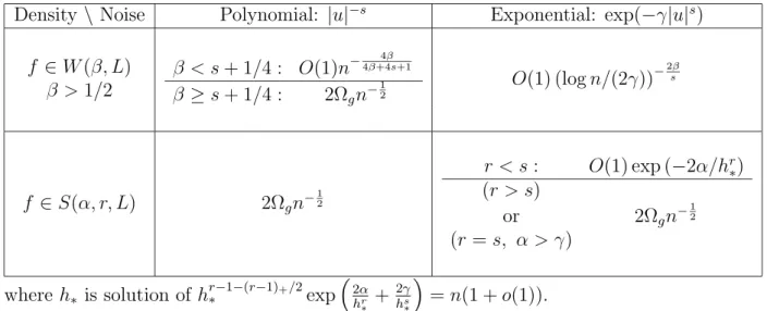
An easy consequence of Proposition 1 is that if the underlying unknown density is smoother enough than the noise (β > s+ 1/4) our parameter can be estimated at parametric rate. We establish next asymptotic normality and a Cramer-Rao type of asymptotic efficiency bound.
Theorem 1 If β > s+ 1/4, the estimator d2
n defined in (11)with bandwidth h =h∗
such that
n−4s1+1 h
∗ n−
1 4β,
is asymptotically normally distributed estimator of d2, i.e.
√
n d2n−d2→d N 0,4Ω2g(f).
Moreover, it attains the asymptotic efficiency Cramer-Rao bound. Proof. Let us decompose the risk of the estimator as follows
Ef[|d2n−d2|]≤B(dn) + p V(dn)≤Lh2β + 2Ωg(f) √ n (1 +o(1)),
and then use Proposition 1. Indeed, ifβ > s+1/4 and ifn−1h−(4s+1) 1 we see that
4Ω2
g(f)/n(1+o(1)) is the dominant term in the variance. Let us takeh=o(n−1/(4β))
such that the bias be infinitely smaller,Lh2β 2Ω
g(f)/n. So,
√
n(d2n−d2) = √n(d2n−Ef[d2n]) +
√
nB(dn).
The second term of the sum in the right-hand side term tends to 0 and the asymptotic normality of the first term can be deduced from Butucea [5]. It is in this case a classical central limit theorem for U-statistics of order 1.
For the Cramer-Rao bound, we follow the lines of proof in Laurent [23]. Similar results were given by Bickel and Ritov [2] following the theory by Ibragimov and Hasminski [18] and Khoshevnik and Levit [22]. A first step of the proof is to compute the Fr´echet derivative of the functional R f2 =R F ·p at likelihood p
0 =f0? g: Z F ·p− Z F0·p0 = Z 2F0(p−p0) + Z (F −F0)(p−p0)
andR(F−F0)(p−p0) = o(kp−p0k2), whenkp−p0k2 →0. Next, consider the space
orthogonal to the square root of the likelihood √p0, H ={k :
Z
k√p0 = 0}
and the projection operator unto this space:
PH(p0)(k) = k−(
Z
k√p0)√p0.
Write Kn = K = T0(p0)√p0 = PH(p0)(k) as hg, ki. Then the minimal variance is
given by kgk2 2. Here,T0(p 0)k = R 2F0k, then K = Z 2F0√p0(k−( Z k√p0)√p0) = Z (2F0√p0)k− Z 2F0p0 Z √p 0k. So, finally, kgk22 = 4 Z |F0|2p0− Z 2F0p0 2 = 4Vf0(F0(Y)).
In the following theorem we compute the rate on the nonparametric side (1/2< β ≤ s + 1/4). We prove in Section 3 that this rate is optimal in the minimax approach under the following additional assumption on the noise distribution.
Assumption (P)The distribution of the polynomial noise in (4) is such that Φg is
at least 3 times continuously differentiable and Φg is at least 2 times continuously
differentiable. Moreover there exist A1, A2 > 1, u0, u1, u2 >0 large enough such
that
|Φg(u)| ≥u0, ∀|u| ≤A1 and |(Φg)(k)(u)| ≤ uk
|u|s+k, for k = 1,2, ∀|u| ≥A2. Theorem 2 If 1/2 < β ≤ s + 1/4, the estimator d2
n of d2 defined in (11) with
bandwidth h∗ satisfies the upper bound (8) for the rate ϕn, where
h∗ =n−4β+42s+1, ϕ
n =n− 4β
4β+4s+1. Moreover, under Assumption (P) this rate is minimax.
Proof of (8). If 1/2< β≤s+ 1/4,kpk2
2/(π(4s+ 1)n2h4∗s+1) is the dominant term in the variance no matter whether β ≥ s or β < s. The bandwidth h∗ minimizes the bias plus the variance. The upper bound of the normalized mean error is less than C= max{L,p2Mp/(π(4s+ 1)}, see Lemma 6.
Remark 2In view of Butucea [5], we get asymptotic normality of the estimatord2
n
defined in (11) in the case 1/2< β < s+ 1/4, for h such that
h =o(1)n−4s1+1 and h=o(1)n− 2 4β+4s+1
(i.e. the variance tends to 0 and the bias is infinitely smaller than the variance, when n→ ∞), nh2s+1/2 d2 n(h)−d2 d →N 0, 2kpk 2 2 π(4s+ 1) .
We will actually use the following type of result for the testing problem
nh2∗s+1/2 dn2 −Ef[d2n] d →N 0, 2kpk 2 2 π(4s+ 1) ,
for the optimal bandwidth h∗ defined in Theorem 2.
2.2
Supersmooth densities and polynomial noise
In the case of supersmooth densities, always smoother than the polynomial noise, we can always define the functionF as the inverse Fourier transform of Φ/Φg. Next
Theorem gives us the right choice of the bandwidth so thatd2
nbe an asymptotically
normal and efficient estimator.
Theorem 3 The estimator d2
n defined in (11) with bandwidth h∗ such that
h∗
logn
4α
−1/r
is asymptotically normally distributed and it attains the asymptotic efficiency
Cramer-Rao bound 4Ω2
g, (see Definition 3).
Proof. In this case, the bias changes,
B(dn)≤Lexp
−2hαr
.
The variance is strongly dependent on the noise distribution, so very little is changed. In this case, the underlying density is always much more regular than the noise, so the function F always exists in this setup. So, we can put together (14) and (17)
V(dn) = 4Ω2 g(f) n (1 +o(1)) + 2kpk2 2 n2h4s+1 (1 +o(1)) π(4s+ 1).
It is obvious that we need to choose h∗ =o(1)(logn/(4α))−1/r, in order to have the squared bias infinitely smaller than the dominant term of the variance 1/n.
2.3
Sobolev densities and exponential noise
In this setup the noise is much smoother so estimation is always difficult, i.e. at nonparametric slower rates. We prove the lower bounds (9), under the following additional assumption, which is not very restrictive.
Assumption (E) The exponential noise distribution in (5) has a continuously dif-ferentiable Fourier transform such that
|Φg(u)| ≤O(1)|u|Aexp(−γ|u|s),
for large enough |u| and some fixed constant A ∈R.
Theorem 4 The estimator d2
n of d2 defined in (11) with bandwidth h∗ satisfies the
upper bound (8) for the rate ϕn, where
h∗ = logn 2γ − 2β+ 1 2γs log logn 2γ −1/s , ϕn =L logn 2γ −2β s . Moreover, under Assumption (E) this rate is minimax.
Proof of (8). In this case, the bias is the same as in Proposition 1,B(dn)≤Lh2β.
As for the variance, we can still writeV(dn) =Ef[|S1|2] +Ef[|S2|2], but both terms
are different now, since they are highly dependent on the noise distribution. We still have, Ef[|S1|2] = 2 +o(1) n(n−1) kpk2 2 h kMnk 2 2, see (15). Now, kMnk22 = h 2π Z |h|≤1/h e4γ|u|sdu= h s 4πγse 4γ hs(1 +o(1)), ash→0, and then Ef[|S1|2] = (2 +o(1))kpk2 2 4πγs hs−1 n2 e 4γ hs. (19)
The other term, can never be of parametric order anymore, the function F never exists in this setup. Indeed, recall that
Ef[|S2|2] ≤ c1 nEf " Z eiuY1Φ K(hu) Φg(u) Φ(u)du 2# (20) ≤ c1 n Z Φ K(hu) Φg(u) Φ(u) du 2
and this integral does not check the Lebesgue convergence theorem anymore. We can compute the rate of divergence, giving a loss in the rate, via Cauchy-Schwarz
Z Φ K(hu) Φg(u) Φ(u) du 2 ≤ Z |Φ(u)|2|u|2βdu Z |u|≤1/h| u|−2βe2γ|u|s du≤c2h2β+s−1e 2γ hs. (21) From (19),(20) and (21), we get
V(d2n)≤C1 hs−1 n2 e 4γ hs(1 +o(1)) +C2h 2β+s−1 n e 2γ hs, (22)
wherec1, c2, C1, C2 >0 are some constants.
As in Theorem 2 we actually select the bandwidth by minimizing an upper bound of the error: Ef[|d2n−d2|]≤ Ef[|d2n−d2|2] 1/2 ≤ B2(dn) +Vf[dn] 1/2 .
The optimality of this upper bound is proven by the corresponding lower bounds. Now, we consider h∗ = arg inf h>0 L2h4β +c2 h2β+s−1 n exp 2γ hs then h∗ is a solution of the equation
h2∗β+1 = c nexp 2γ hs ∗ (1 +o(1)). (23) This proves that the bias is infinitely larger than the variance and gives announced
h∗ and rate of order of the bias ϕn. (If we suppose that the first term on the
right-hand side of (22) is dominant, we get a contradiction).
2.4
Supersmooth densities and exponential noise
In this setup unknown densities and noise densities are both exponentially smooth. Note that minimax rates in the nonparametric ”regime” are faster than any loga-rithm but slower than any polynomial of n.
Theorem 5 If r > s or, if r=s and α > γ, the estimator d2
n defined in (11) with
bandwidth h∗ such that
h∗
logn
4α
−1/r
is asymptotically normally distributed and it attains the asymptotic efficiency
Cramer-Rao bound 4Ω2
g.
If r < sthe same estimator d2
n of d2 with bandwidthh∗ satisfies the upper bounds
(8) for the rate ϕn, where
h∗ solution of hr−1−(r−1)+/2 ∗ exp 2α hr ∗ + 2γ hs ∗ =cn(1 +o(1)), ϕn=Lexp −2hαr ∗ . Moreover, unde Assumption (E) this rate is minimax.
Proof. We skip the proof of asymptotic efficiency. If r < s, we know the bias is
B(d2
n)≤Lexp (−2α/hr) and the variance writes also Vf[d2n] = Ef[|S1|2] +Ef[|S2|2].
Furthermore,Ef[|S1|2] is the same as in (19).
As in (20), we need to study Z |u|≤1/h eiuY1 Φ(u) Φg(u)du 2 .
If r > s or, if r = s and α > γ, this integral is bounded by a constant depending only on α, r, L and the noise density g. So, the variance
Vf[Tn∗2] =Ef[|S2|2](1 +o(1)) =
4Ω2
g(f)
n (1 +o(1)),
as soon ashs−1n−1exp(4γ/hs) =o(1). For the bandwidth we chose in the theorem,
this holds and proves this case. If r < s, Z |u|≤1/h eiuY1 Φ(u) Φg(u)du 2 ≤ Z e2α|u|r|Φ(u)|2du Z |u|≤1/h e−2α|u|re2γ|u|sdu ≤ c1hs−1exp 2γ hs − 2α hr . Thus, Vf[d2n]≤c1 hs−1 n exp 2γ hs − 2α hr +c2 hs−1 n2 exp 4γ hs ,
where c1, c2, . . . are some positive constants. As in Theorems 2 and 4 we find the
optimal bandwidth by minimizing an upper bound of the error
h∗ = arg inf h>0 L2exp −4α hr +c1 hs−1 n exp 2γ hs − 2α hr +c2 hs−1 n2 exp 4γ hs .
When we minimize the sum of the bias and of the first term in the variance, we find that h∗ is solution of the equation
hr∗−1exp 2α hr ∗ +2γ hs ∗ =cn(1 +o(1)).
It implies that the first term in the variance is dominant over the second, if r <1, meaning, moreover that
L2exp −4α hr ∗ =hr∗−sc2 hs−1 ∗ n exp 2γ hs ∗ − 2α hr ∗
If we minimize the sum of the bias and the second term in the variance, we find that optimal bandwidth h∗ verifies
h(∗r−1)/2exp 2α hr ∗ +2γ hs ∗ =cn(1 +o(1)).
The second term of the variance is dominant if r≥ 1 and in this case also the bias is dominant over the variance forr < s and the optimal h∗, respectively, the bias is of the same order as the dominant term in the variance, if r =s and α < γ. This finishes the proof of the Theorem.
Remark 3: More upper boundsLet us add upper bounds of the estimation risk in cases not included in the Theorem. We put them aside since we do not provide corresponding lower bounds in these cases.
In the case r =s and α < γ, the same choice of the bandwidth holds as in the case r < s of the preceding Theorem. The bias is in this case of the same order as the dominant term in the variance (not larger than the variance).
If r=s and α=γ, Vf[d2n]≤ c1 nh+c2 hs−1 n2 exp 4γ hs .
In this case, the first term in the upper bound of the variance is always dominating over the second and when we minimize the sum of this term and of the bias we get an optimalh∗ solution of hr∗−1exp 4α hr ∗ =cn(1 +o(1)),
giving a fast rate of convergence of the order of the variance:
ϕ2n=c3
(logn)r
n .
3
Goodness-of-fit tests
Let us construct a test statistic from noisy data. It is natural to suggest as a test statistic Tn∗, the square root of the optimal estimator of the quadratic functional
kf−f0k22: Tn∗2 = 1 n(n−1) X k6=j hKn,h(· −Yk)−f0, Kn,h(· −Yj)−f0i,
whereh >0, h→0 andKn,h = 1/hKn(·/h), for the same Kn defined in (10).
Define the test procedure ∆∗n= 1 T∗2 n >C∗t2n 0 T∗2 n ≤ C∗t2n (24) for a constant C∗ >0 and some threshold t
Density \ Noise Polynomial: |u|−s Exponential: exp(−γ|u|s) f ∈W(β, L) β >1/2 β < s+ 1/4 : O(1)n−4β+44βs+1 β ≥s+ 1/4 : 2Ωgn− 1 2 O(1) (logn/(2γ))−2sβ f ∈S(α, r, L) 2Ωgn− 1 2 r < s: O(1) exp (−2α/hr ∗) (r > s) or 2Ωgn− 1 2 (r =s, α > γ) whereh∗ is solution ofhr−1−(r−1)+/2 ∗ exp 2α hr ∗ + 2γ hs ∗ =n(1 +o(1)). Table 1: Estimation rates ofd2 from noisy data
3.1
Sobolev densities and polynomial noise
Though two rates were attainable in the same setup for estimating d2, only one
minimax rate of testing is possible. This phenomenon is similar to the case of testing with direct observations.
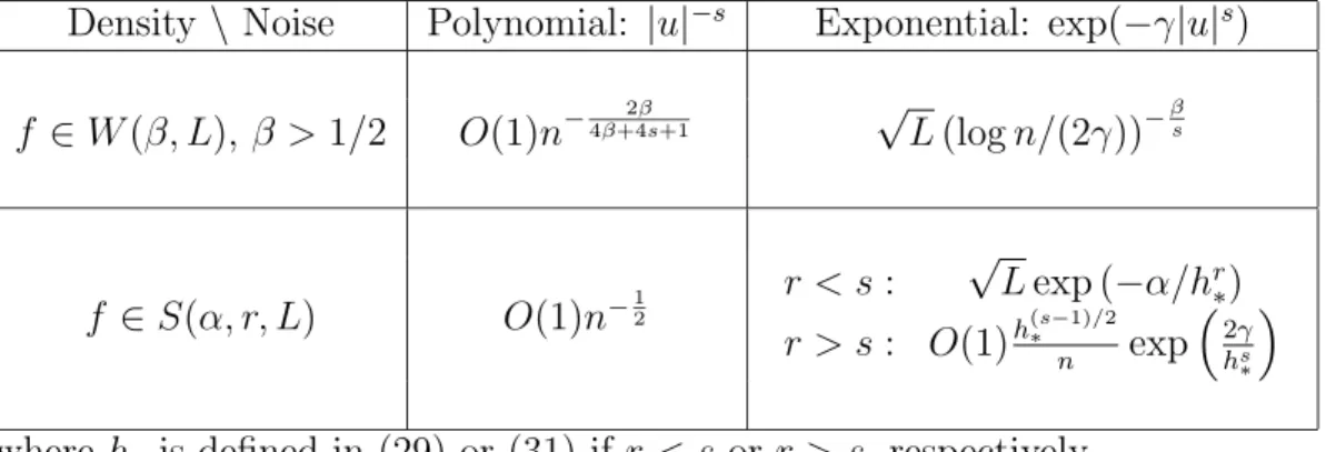
Theorem 6 The test procedure ∆∗
n defined in (24) for the threshold tn attains the
rate ψn and, under Assumption (P), ψn is a minimax rate of testing over the class
W(β, L), where
h=h∗ =n−4β+42s+1, t
n =ψn=n− 2β
4β+4s+1.
Proof of upper bounds (6). Let us bound from above successively the first and second type error. Note that, for a fixed density f0 ∈W(β, L):
Ef0[T
∗2
n ] =kKh? f0−f0k22 =Lh2βo(1),
similarly to the proof of Proposition 1. In order to compute the variance let us write as follows Tn∗2−Ef0[T∗ 2 n ] = 1 n(n−1) X k6=j hKn,h(· −Yk)−f0, Kn,h(· −Yj)−f0i − kKh? f0−f0k22 = 1 n(n−1) X k6=j hKn,h(· −Yk)−Kh? f0, Kn,h(· −Yj)−Kh? f0i +2 n n X k=1 hKn,h(· −Yk)−Kh? f0, Kh? f0−f0i.
Note that, for allk = 1, . . . , n, hKn,h(· −Yk)−Kh? f0, Kh? f0−f0i = 1 2π Z ΦKn(hu)eiuYk−ΦK(hu)Φ 0(u) ΦK(hu)−1Φ0(u)du = 1 2π Z ΦK(hu) ΦK(hu)−1 eiuYk/Φg(hu)−Φ 0(u) Φ0(u)du= 0,
due to the support of ΦK. Finally,
Vf0[T∗ 2
n ] = Ef0[|S1|
2] = Skp0k22
n2h4s+1(1 +o(1)),
whereS = 2/(π(4s+ 1)). So the first type error can be written as follows
Pf0[T ∗2 n ≥ C∗t2n] = Pf0[T ∗2 n −Ef0[T ∗2 n ]≥ C∗t2n−c1h2β] = O(1) n− 2h−(4s+1) (C∗t2 n−c1h2β)2 ≤ α 2 since, forh=h∗ 1 nh2s+1/2 ≤O(1) max{t 2 n, h2β}. (25)
For the second type error, consider a density f in H1(C, ψn). Then, Ef[Tn∗2] =
kKh? f −f0k22.The bias can be bounded from above as follows B[Tn∗2] = |kKh? f −f0k22− kf−f0k22| = |kKh? fk22− kfk22−2hKh? f −f, f0i| ≤ 1 2π Z |u|>1/h| Φ(u)|2du+ 2 2π Z |u|>1/h| Φ(u)| · |Φ0(u)|du ≤ Lh2β(1 +o(1)), since R|u|>1/h|u|2β|Φ
0(u)|2du = o(1), for the fixed density f0. In order to evaluate
the variance, let us decompose as follows
Tn∗2−Ef[Tn∗2] = 1 n(n−1) X k6=j hKn,h(· −Yk)−f0, Kn,h(· −Yj)−f0i − kKh ? f −f0k22 = 1 n(n−1) X k6=j hKn,h(· −Yk)−Kh? f, Kn,h(· −Yj)−Kh ? fi +2 n n X k=1 hKn,h(· −Yk)−Kh? f, f−f0i = S1(f) +S2(f −f0),say.
As in Proposition 1, the last two terms are uncorrelated, soVf[Tn∗2] = Ef[|S1(f)|2] + Ef[|S2(f−f0)|2]. Similar computation lead to
Vf[Tn∗2] ≤ C1 n2h4s+1 + (4 +o(1))Ω2 g(f −f0) n I(β > s) + C3 nh2(s−β)I(β ≤s) ≤ C1 n2h4s+1 + C2kf −f0k22 n I(β > s) = Def v2 n.
Indeed, let us see that whenever β > s, we findM > 0 large enough such that Ω2g(f−f0) ≤ Z (F(y)−F0(y))2p(y)dy≤ kF −f0k2∞ ≤ 1 4π2 Z Φ(uΦ)−g(uΦ)0(u) 2 du ≤ Z |u|≤M c1M2s|Φ(u)−Φ0(u)|2du+ Z |u|>M c2|u|2s|Φ(u)−Φ0(u)|2du ≤ c3kf −f0k22+ c2 M2(β−s) Z |u|>M| u|2β|Φ(u)|2du≤Ckf −f0k22, (26)
where, C is a constant depending only on β, L and of the fixed noise probability densityg. We also use the fact that for h=h∗,
1 nh2(s−β)/ 1 n2h4s+1 =n−4β+41s+1 =o(1).
So, the second type error can be bounded as follows
Pf[Tn∗2 <C∗t2n] = Pf[Tn∗2−Ef[Tn∗]<C∗t2n−Ef[Tn∗] +kf −f0k22− kf−f0k22] ≤ Pf[Tn∗2−Ef[Tn∗]<−kf−f0k22+C∗t2n+B[Tn∗2]] ≤ Pf " T∗2 n −Ef[Tn∗] p Vf[Tn∗2] ≤ −kf−f0k 2 2+C∗t2n+B[Tn∗2] vn # , (27) forn large enough. From Butucea [5] we deduce easily the asymptotic normality of center and reduced T∗2
n . The proof is based on a result by Hall [17] for U-statistics
of order 2 adapted for the case of noisy observations.
So the last probability in (27) is smaller than α/2 +o(1) if −kf−f0k22+C∗t2n+B[Tn∗2] C1 n2h4s+1 + C2kf−f0k22 n I(β ≥s) 1/2 ≤ −z1−α/2, (28)
where zp denotes the p-quantile of the standard gaussian law N(0,1). So, either β ≤s, then −kf −f0k22 +C∗t2n+B[Tn∗2] C1 n2h4s+1 + C2kf−f0k22 n I(β > s) 1/2 ≤ −C∗ψ2 n+C∗t2n+B[Tn∗2] n−1h−(2s+1/2) ,
which is smaller than −z1−α/2 for ψn = tn verifying (25). Or, β > s, then we can
solve
−kf −f0k22+C∗t2n+B[Tn∗2] C4kf−f0k2/√n ≤ −
z1−α/2
and (use also (25)) find
kf −f0k2 ≥ C4z1−α/2 2√n + 1 2 s C2 4z12−α/2 n + 4(C∗t 2 n+B[Tn∗2]) ≥ max ( C5 √ n, C6 C7 n2h4s+1 +Lh 2β 1/2) ≥ C1/2ψ n,
for C∗ large enough, since h = h∗ minimizes the risk C7n−2h−(4s+1) +Lh2β. The
upper bounds in (6) are proven. For the lower bounds in (7) see Section 3.
3.2
Supersmooth densities and polynomial noise
Very surprisingly, in this setup, we can estimated2 at parametric rate, moreover we
can also provide minimax testing at parametric n−1/2 rate. Theorem 7 The test procedure ∆∗
n defined in (24) for the threshold tn attains the
rate ψn and ψn is a minimax rate of testing over the class S(α, r, L), where
h=h∗ logn 4α −1/r , tn=ψn =n− 1 2.
Proof. We follow the lines of proof in Theorem 6, using computation from the proof of Theorem 3 in this setup. For the first type error see that
Ef0[T∗ 2 n ] = o(1)Le−2α/h r and Vf0[T∗ 2 n ] = Skp0k22 n2h4s+1(1 +o(1)),
wherep0 =f0∗g. Using Markov’s inequality Pf0[T∗ 2 n ≥ C∗t2n]≤ Cn−2h−(4s+1) (C∗t2 n−o(1) exp(−2α/hr))2 =o(1),
since max{n−2h−(4s+1),exp(−2α/hr)}=o(t2
n).
For an arbitrary density f ∈H1(C, ψn),
B[Tn∗2] =|kKh? f −f0k22− kf −f0k22| ≤Lexp(−2α/hr)(1 +o(1))
and Vf[Tn∗2] ≤ C1kf −f0k22/n =Def vn. Indeed, similarly to the proof in (26), we
have for some M >0 large enough Ω2g(f−f0)≤c1kf −f0k22+c2e−2αM
rZ
|u|>M
e2α|u|r|Φ(u)|2du≤C
where C1 > 0 depends only on α, r, L and the noise fixed probability density g.
Using the asymptotic normality of this U-statistic of order 2, we get
Pf[Tn∗2 <C∗t2n]≤Pf " T∗2 np−Ef[Tn∗2] Vf[Tn∗2] ≤ −kf −f0k 2 2 +C∗t2n+B[Tn∗2] C11/2kf−f0k2/√n # ≤ α 2 +o(1), if −C1−1/2kf −f0k2 √ n+C1−1/2√n(C∗t2 n+B[Tn∗2])≤ −z1−α/2. We actually have −C1−1/2kf −f0k2√n+C1−1/2 √ n(C∗t2n+B[Tn∗2])≤ −(C/C1)1/2+o(1)
which is less than the needed quantile forC >C∗ large enough.
3.3
Sobolev densities and exponential noise
Theorem 8 The test procedure ∆∗n defined in (24), for the threshold tn and for the
constant C∗ = 1, attains the rate ψ
n and, under Assumption (E), ψn is an exact
minimax rate of testing over the class W(β, L), where
h=h∗ = logn 2γ − 2β+ 1 2γs log logn 2γ −1/s , tn=ψn = √ L logn 2γ −β/s . Proof. Again, under the null hypothesis and h=h∗
Ef0[T∗ 2 n ] = Lh2βo(1), Vf0[T∗ 2 n ] = Ef0[|S1| 2] ≤c1 hs−1 n2 exp 4γ hs .
The first type error can be bounded then:
Pf0[T ∗2 n ≥ C∗t2n]≤ c1hs−1n−2exp(4γ/hs) (C∗t2 n−Lh2β)2 ≤c2hs∗+1 =o(1),
where we used the facts that C∗ = 1, that t2
n ≤Lh2β and that h =h∗ is solution of
(23), i.e. n−2exp(4γ/hs) = c−2h−4β−2. Under the alternative, if f ∈H
1(C, ψn): Bf[Tn∗2]≤Lh2β(1 +o(1)), Vf[Tn∗2]≤c3 h2β+s−1 n exp 2γ hs =c4h4β+s,
where we used again (23). Then for C =C∗(1 +δ)>C∗, δ >0, we have
Pf[Tn∗ <C∗t2n] ≤ Pf " Efp[Tn∗2]−Tn∗2 Vf[Tn∗2] ≥ −C∗t 2 n−Bf[Tn∗2] +kf −f0k22 √c 4h2∗β+s/2 # ≤ Pf " Ef[Tn∗2]−Tn∗2 p Vf[Tn∗2] ≥ C∗δψ 2 n−Lh2∗β(1 +o(1)) √c 4h2∗β+s/2 # ≤ c5hs∗ =o(1),
3.4
Supersmooth densities and exponential noise
Unknown densities and noise densities are both supersmooth. Nevertheless, there is an essential difference with the case of Sobolev densities and polynomial noise from Subsection 3.1. Nonparametric minimax rates of testing are faster whenr > s than in the case r < s.
3.4.1 Case r < s
Theorem 9 The test procedure ∆∗
n defined in (24), for the threshold tn and for the
constant C∗ = 1, attains the rate ψ
n and, under Assumption (E), ψn is an exact
minimax rate of testing over the class S(α, r, L), where
h =h∗ = is a solution of hr−1−(r−1)+/2 ∗ exp 2α hr ∗ +2γ hs ∗ =n(1 +o(1)),(29) tn = ψn = √ Lexp −hαr ∗ .
Proof. Under the null hypothesis and for h=h∗
Ef0[T ∗2 n ] = o(1)Le−2α/h r , Vf0[T ∗2 n ]≤c1 hs−1 n2 exp 4γ hs . (30)
Then the first type error is bounded by
Pf0[T ∗2 n ≥ C∗t2n]≤ c1hs−1n−2exp(4γ/hs) (C∗t2 n−Lexp(−2α/hr))2 ≤c3h2−2r−(r−1)++s−1 =o(1),
where we used the facts that h = h∗ is defined by (29) and that r < s. Under the alternative, use Theorem 7
Bf[Tn∗2]≤Le−2α/h r (1+o(1)), Vf[Tn∗2]≤c1 hs−1 n exp 2γ hs − 2α hr +c2 hs−1 n2 exp 4γ hs .
For C = C∗(1 +δ) > C∗, δ > 0, use Theorem 5 saying that, for h = h
∗ defined in (29), ψ2
n = t2n are of the same order as exp(−4α/hr) which is infinitely larger than
p Vf[Tn∗2] to get Pf[Tn∗2 <C∗t2n] ≤ Pf " Efp[Tn∗2]−Tn∗2 Vf[Tn∗2] ≥ −C∗t 2 n−Bpf[Tn∗2] +kf−f0k22 Vf[Tn∗2] # ≤ Pf " Efp[Tn∗2]−Tn∗2 Vf[Tn∗2] ≥ C∗δψ 2 n−Lexp(p −4α/hr)(1 +o(1)) Vf[Tn∗2] # ≤ Vf[T∗ 2 n ] c4exp(−4α/hr) =o(1), by Markov’s inequality.
3.4.2 Case r > s
Note that no lower bounds are provided for this setup. Nevertheless, we expect the rates to be optimal in the minimax sense.
Theorem 10 The test procedure ∆∗n defined in (24) for the threshold tn is a test
procedure attaining the rate ψn over the class S(α, r, L), (see (6)), where
h =h∗ = is a solution of h(∗r−1)/2exp 2α hr ∗ +2γ hs ∗ =n(1 +o(1)), (31) tn = ψn = h(∗s−1)/2 n exp 2γ hs ∗ .
Proof. Under the null hypothesis, (30) still holds. Forh =h∗ defined in (31),tn is
of the order ofh(s−1)/2n−1exp(2γ/hs) and the bias exp(−2α/hr) =c
2hr−stn=o(tn).
Thus, the first type error is smaller than α/2 for someC∗ large enough. Under the alternative,
Bf[Tn∗2]≤Le−2α/h r (1 +o(1)), Vf[Tn∗2]≤ 4Ωg(f −f0) n +c2 hs−1 n2 exp 4γ hs
and we can prove as in Theorems 6 and 7 that 4Ωg(f −f0) ≤ C1kf −f0k22. Then
the second type error is bounded by α/2 +o(1) as soon as −kf −f0k22+C∗t2n+Lexp(−2α/hr) (C1kf−f0k22/n+c2hs−1n−2exp(4γ/hs))1/2 ≤ − z1−α/2. This is equivalent to kf −f0k2 ≥max 1 √ n, h(s−1)/2 n e 2γ/hs +Le−2α/hr ,
sinceh=h∗defined by (31) minimizes the sum on the right-hand side of the previous inequality. As a result ψn =c3 h(s−1)/2 n e 2γ/hs =h(s−r)/2e−2α/hr
which is infinitely smaller than the bias. Note that, the rate is indeed slower than any polynomialn−a, a >0 but faster than any logarithmic rate.
4
Lower bounds
We show in a first part that proofs for minimax lower bounds for the estimation problem of d2 and for the testing problem in L2 come down to the same choice of
Density \ Noise Polynomial: |u|−s Exponential: exp(−γ|u|s) f ∈W(β, L), β >1/2 O(1)n−4β+42βs+1 √L(logn/(2γ))− β s f ∈S(α, r, L) O(1)n−12 r < s: √Lexp (−α/hr ∗) r > s: O(1)h(∗s−1)/2 n exp 2γ hs ∗
whereh∗ is defined in (29) or (31) if r < s orr > s, respectively. Table 2: Testing rates in L2-norm from noisy data
Let us define Rest := inf ˆ d2 n sup f∈W(β,L) ϕn−1Ef[|dˆ2n−d2|] Rtest := inf ∆n sup f∈W(β,L) PH0(∆n= 1) +PH1(C,ψn)(∆n= 0) .
Lemma 1 Letf0 andf1 be two probability densities in the classW(β, L), depending
on n, and denote by PY
0 , E0 and P1Y, E1 the probability measures of our data and
the expected value when the true underlying parameters are f0 and f1, respectively.
If
a) estimation problem densities are such that |kf1k22 − kf0k22| ≥ 2ϕn, for some ϕn >0,
a0) test problem densities are such that kf
1 −f0k2 ≥ Cψn, for some ψn >0,
b) P1 P0 and there exists 0< γ <1 such that
χ2(P0, P1) :=Def Z dP1 dP0 − 1 2 dP0 ≤γ2 then Rest ≥ (1−γ)(1−√γ) (32) Rtest ≥ (1−γ)(1−√γ). (33)
Proof. For the estimation problem we reduce the risk to two hypothesis:
Rest≥inf ˆ d2 n max i=0,1ϕ −1 n Efi[|dˆ 2 n−d2i|],
and then use directly Lemma 4 from Butucea and Tsybakov [6], adapted from Tsybakov [37].
For the testing problem, we choose two hypothesesf0 the density under H0 and
another densityf1 underH1(which implies thatkf1−f0k2 ≥ Cψn, for someψn>0).
Then the risk for the test problem becomes
Rtest ≥ inf ∆n P0(∆n= 1) + (1−√γ)P0 ∆n= 0, dPY 1 dPY 0 ≥1−√γ ≥ (1−√γ)P0 dPY 1 dPY 0 ≥ 1−√γ ≥ (1−√γ) 1− 1 γE0 " dPY 1 dPY 0 −1 2#! ≥(1−γ)(1−√γ), if Assumption b) holds.
We shall use in the proofs the following construction and Lemma 2. Let 0< δ <1 be small through the remaining proofs of lower bounds. Letf0 be a density function
in the Sobolev class W(β, a(δ)L), respectively,S(α, r, a(δ)L), where 0< a(δ)<1 is a constant depending on δ defined for each setup, such that
f0(x)≥ c0
1 +|x|2, ∀x∈R. (34)
Moreover we want the Fourier transform Φ0 to have compact support included in
(−2δ,2δ).
Let us note immediately that we have a similar property forfY
0 =f0∗g. Indeed,
letA >1 large enough be such that R−AAg(x)dx >1/2, then
f0Y(x)≥ Z A −A f0(x−y)g(y)dy≥cY0 min 1 A2, 1 |x|2 ,∀x∈R, (35) wherecY 0 >0.
Lemma 2 (Lemma 1 in Butucea and Tsybakov [6]) For any δ > 0 and any D >4δ there exists a function ΦG:R →[0,1] such that
(i) ΦG is 3 times continuously differentiable on R and its first 3 derivatives are
uniformly bounded on R,
(ii) ΦG is compactly supported on (δ, D−δ) and
I(2δ,D−2δ)(u)≤ΦG(u)≤I(δ,D−δ)(u),
for all u∈R, where IA(u) denotes the indicator function of the interval A.
Proof of the lower bounds in Theorems 4 and 8. Here we check the assump-tions in Lemma 1 and then (32) and (33) imply the needed results. Let us consider the density functionf0 in the class W(β, a(δ)L) for some small 0< δ <1 such that
Let ΦG be defined by Lemma 2 with D= 1 and the perturbation functionH be
defined via its Fourier transform
ΦH(u, h) =√πLh−βΦ
G(|u| −1/h)
1 +|u|2β ,
whereβ > 1/2 and h→0 as n → ∞.
Then the second hypothesis function f1 is defined as follows f1(x) = f0(x) +H(x, h), forh = logn 2γ − B 2γslog logn 2γ −1/s ,
for some constantB ∈R fixed later on. Note that the characteristic functions verify Φ1(u) = Φ0(u) + ΦH(u, h).
Let us see first that f1 is a probability density function. Indeed, since ΦH(·, h)
is 3 times continuously differentiable, then via integration by parts we get |H(x, h)|= −2πix1 3 Z e−iux(ΦH)000(u)du ≤ 1 +CH|x|3, (36)
for all x∈R, for some constant CH >0. Note also that
kH(·, h)k∞ ≤ 1 2π Z |ΦH(u, h)|du≤ r L π h−β 2 Z δ≤|u|−1/h≤1−δ du 1 +|u|2β ≤ r L πh −β Z 1/h+1 1/h du 1 +u2β ≤ch β, (37)
which is o(1) forβ >1/2 and h→0. Since f0 is such that (34) holds, (36) and (37)
show thatf1 is a non negative function.
Moreover, R f1(x)dx= Φ1(0) = 1 and f1 is a probability density function.
Let us check now that it belongs to the class W(β, L). Indeed, 1 2π Z |ΦH(u, h)|2|u|2βdu ≤ L 2h −2β Z δ≤|u|−1/h≤1−δ |u|2βdu (1 +|u|2β)2 ≤ Lh−2β Z 1/h+1−δ 1/h+δ du u2β ≤ L 2β−1h −2β " 1 h +δ −2β+1 − 1 h + 1−δ −2β+1# ≤ L(1−2δ)(1 +o(1))≤L(1−δ),
for n large enough. So, H belongs toW(β, L(1−δ)), implying that 21π Z |Φ1|2| · |2β 2 ≤ 21π Z |Φ0|2| · |2β 2 + 21π Z |ΦH(·, h)|2| · |2β 2 ≤√L,
for a(δ) = (1−√1−δ)2. Then f
1 ∈W(β, L).
Let us check a), respectively a’) in Lemma 1. Note that Φ0 and ΦH(·, h) have
disjoint supports for allh >0 and then by Plancherel formula kf1k22− kf0k22 =kf1−f0k22 = 1 2π Z |ΦH(u, h)|2du.
Thus, it is enough to deal with kf1−f0k22 = 1 2ππLh −2β Z |ΦG(|u| −1/h)|2 (1 +|u|2β)2 du ≥ L 2h −2β Z 1/h+2δ≤|u|≤1/h+1−2δ du (1 +|u|2β)2 ≥ Lh−2β Z 1/h+1−2δ 1/h+2δ du (1 +u2β)2 ≥ Lh−2β(1−4δ)(1 +o(1)) (1 + (1/h)2β)2 ≥Lh 2β,
for small 0 < δ < 1 and large enough n. Note that this construction provides the right constant for testing, but not for the estimation ofd2.
Let us check b) of Lemma 1. Note first that χ2(P
0, P1) ≤ Cnχ2(f0Y, f1Y), for
some constant C > 0, if nχ2(fY
0 , f1Y) is small. We use again the property (35) of fY 0 : nχ2(f0Y, f1Y) = n Z (fY 1 −f0Y)2(y) fY 0 (y) dy ≤ n cY 0 A2 Z |y|≤A (H(·, h)? g)2(y)dy+ Z |y|>A y2(H(·, h)? g)2(y)dy ≤ cnY 0 A2kH(·, h)? gk22+ n cY 0 Z (ΦH(u, h)Φg(u))02du. (38) On the one hand, let
T1 := nkH(·, h)? gk22 = n 2π Z |ΦH(u, h)Φg(u)|2du ≤ O(1)nh−2β Z 1/h+δ≤|u|≤1/h+1−δ exp(−2γ|u|s) (1 +|u|2β)2 du ≤ O(1)nh−2β Z ∞ 1/h exp(−2γus) (1 +u2β)2 du ≤ O(1)nh2β+s−1exp −2hγs , (39)
for h >0 small enough. On the other hand, under the additional Assumption (E) T2 := n Z (ΦH(u, h)Φg(u))02du ≤ O(1)nh−2β Z ∞ 1/h| u|2Ae−2γ|u|s du ≤ O(1)nh−2β−2A+s−1exp −2hγs , (40)
for some fixedA ∈R. If we choose someB < min{2β+s−1,−2β−2A+s−1}, we conclude from (38), (39) and (40) that
nχ2(fY 0 , f1Y)≤o(1)nhBexp −2γ hs =o(1), by the choice ofh.
Proof of the lower bounds in Theorems 5 and 9. The proof in this case is very similar to the previous one and it can be easily adapted from Butucea and Tsybakov [6] (L2 case). Let us choose f0 such that (34) holds and such that the
support of Φ0 be included in (−2δ,2δ). For ΦGdefined in Lemma 2, letH be defined
via its Fourier transform
ΦH(u, h) = p2παrL(d−1)h(1−r)/2e(d−1)α/hrexp(−αd|u|r)ΦG(|u|r−1/hr),
where d=δ−1/2 and D =D(δ)→ ∞ as δ →0, such that Dδ →0. We know then,
that f1 =f0+H(·, h) belongs to S(α, r, L) as soon as a(δ)<(1−e−α(d−1)δ)2.
We can actually consider hsolution of the equation
nexp
−2hαr − 2hγs
= exp(−(log logn)2).
Then, kf1k22 − kf0k22 =kf1−f0k22 ≥Lexp −2hαr (1−√δ)[e−4α√δ−e−2α(D−2δ)/√δ](1+o(1)),
asn→ ∞. It is easy to prove thatLexp(−2α/hr) =Lexp(−2α/hr
∗)(1+o(1)), where
h∗ is defined in (29). This means we checked a) and a’) in Lemma 1. Following the same ideas as in the previous proof, under the additional Assumption (E), there exists someB ∈R fixed such that b)of Lemma 1:
nχ2(f0Y, f1Y)≤o(1)nhBexp −2α hr − 2γ hs ≤o(1) by the choice ofh. Again, this proof gives exact minimax testing rates.
Proof of the lower bounds in Theorems 2 and 6. This proof is based on a large family of hypotheses. A similar reasoning proves that the same construc-tion is valid for proving lower bounds for both quadratic funcconstruc-tional estimaconstruc-tion and nonparametric testing in L2.
Note that this setup includes Theorem 2 for β < s+ 1/4. This is not a contra-diction, since the lower bounds here are much slower than the parametricn−1/2 rate
that the estimator attained, see Theorem 1.
Let θj, j = 1, . . . , M, be independent Bernoulli random variables and let Π be
the probability measure associated to them. For h > 0 small as n → ∞ and for a functionH to be defined later, let
fθ(x) = f0(x) +
M
X
j=1
θjhβ+s+1Hh(x−xj), (41)
where Hh(·) = 1/hH(·/h), xj =jh and M is an integer such that M/h= 1−o(1),
asn → ∞andhsmall. Note that observationsYi,i= 1, . . . , n, when the underlying
density is fθ, have density
fθY(x) =f0Y(x) +
M
X
j=1
θjhβ+s+1Gh(x−xj), (42)
where the functionG is defined in Lemma 3 and H is such that ΦG(u) = ΦH(u)Φgu h . (43) Indeed, (Hh(· −xj)∗g) (x) = Hh∗g(x−xj) =Gh(x−xj).
Using Lemmas 4 and 5, we see that the hypotheses fit into the model, i.e. fθ are
density functions for all θ, belonging to the Sobolev class W(β, L) and such that Πkfθ−f0k22 ≥ Cn−4β/(4β+4s+1)
→1,
asn → ∞, for fixedc > 0.
Lemma 3 Let the function G: [−1,0]→R be defined by G(x) = exp − 1 1−(4x+ 3)2 I(−1≤x≤ −1/2)−exp − 1 1−(4x+ 1)2 I(−1/2< x≤0).
Then G is an infinitely differentiable function, such that R G(x)dx = 0 and having
all polynomial moments finite. Its Fourier transform is such that
|ΦG(u)| ≤CGexp(−a
p
|u|), as |u| → ∞,
for some positive constants CG, a >0. Moreover ΦG is an infinitely differentiable,
This construction is based on the function fa in Lepski and Levit [24], p. 133 and
the asymptotic behaviour of its Fourier transform follows from the reference therein. All other statements have classical proofs for Fourier and inverse Fourier transforms of functions in L1 and L2.
We stress the fact that in this setup, hypotheses functionsfθ belong toH1(C, ψn)
with probability which tends to 1 when n→ ∞. In order to bound from below the risk, very small modification is needed in the proof of Lemma 1 that we do not discuss in detail here. The last thing to check is that the distance between resulting models is finite: ∆2 := Ef0 "R Qn i=1fθY(Yi)π(dθ)−Qni=1f0Y(Yi) Qn i=1f0Y(Yi) 2# = Ef0 Z n Y i=1 fY θ fY 0 (Yi)π(dθ) !2 −1 = Ef0 Z n Y i=1 1 + M X j=1 θjhβ+s+1 Gh(Yi−xj) fY 0 (Yi) ! π(dθj) !2 −1.
Now, callYi,j those observationsYi belonging to the support ofGh(· −xj) and since
those intervals are disjoint we write ∆2 = Ef0 Z n Y i=1 M Y j=1 1 +θjhβ+s+1 Gh(Yi,j −xj) fY 0 (Yi,j) π(dθj) !2 −1 = M Y j=1 Ef0 Z n Y i=1 1 +θjhβ+s+1 Gh(Yi,j −xj) fY 0 (Yi,j) π(dθj) !2 −1 ≤ M Y j=1 ( 1 2 1 +h 2β+2s+2E " Gh(Y1,j−xj) fY 0 (Y1,j) 2#!n +1 2 1−h 2β+2s+2E " Gh(Y1,j−xj) fY 0 (Y1,j) 2#!n) −1,
where we used the facts that (a+b)2 ≤2a2+ 2b2 and that R G= 0 giving E Gh(Y1,j −xj) fY 0 (Y1,j) = 0.
Use Lemma 5 and expressions ofM and h inn to get ∆2 ≤ 1 +c3n2 h2β+2s+2E " Gh(Y1,j−xj) fY 0 (Y1,j) 2#!2 M −1 ≤ c4M n2h4β+4s+2 ≤c5.
Lemma 4 For all θ ∈ {−1,1}M and for h > 0 which tends to 0 as defined Theo-rems 2 and 6, then
1. the functions fY
θ given by (42), with G defined in Lemma 3 are probability
density functions, i.e. non-negative functions of integral equal to 1,
2. the functionsfθ given by (41), with H defined by (43) and Lemma 3 are
prob-ability density functions, given Assumption (P) and that Φg(u) 6= 0 for all
u∈R.
Proof. 1. It is easy to see that R fY
θ (x)dx = 1, since
R
G(x)dx = 0 and fY
0 is
a probability density function, positive on R. We have to check that fY
θ is
non-negative on [0,1]. For all j = 1, . . . , M and for x in the support of the function
Gh(· −xj) we have fθY(x) = f0Y(x) +θjhβ+s+1Gh(x−xj). Then fθY(x)≥ inf 0≤x≤1f Y 0 (x)−hβ+ssup x | G((x−xj)/h)| ≥cY −o(1)>0,
for n large enough.
2. Let us note first that ΦH(0) = ΦG(0)/Φg(0) = 0, implying thatR H(x)dx= 0.
Moreover, ΦH is in L
1 andL2, uniformly continuous function. Then
R
fθ(x)dx= 1.
In order to study its positivity, we use two methods. First, for x small enough we use hβ+s+1|Hh(x)| ≤ hβ+s+1 1 2π Z Φ G(hu) Φg(u) du ≤ hβ+s+1 1 2π Z |u|≤A u−01|ΦG(hu)|du+ Z |u|>A c3|u|s|ΦG(hu)|du ≤ c4hβ+s Z |v|≤Ah| ΦG(v)|dv+c5hβ Z |v|>Ah| v|s|ΦG(v)|du≤c6hβ(44),
for A > max{A1, A2} large enough (see Assumption (P)). For x large, we need a
sharper bound that we get using derivability and boundedness properties of ΦG
hβ+s+1|Hh(x)| = hβ+s+1 1 2π Z e−ixuΦ G(hu) Φg(u) du = hβ+s+1 exp(−ixu) −2πix ΦG(hu) Φg(u) ∞ −∞ + 1 2πix Z e−ixu ∂ ∂u ΦG(hu) Φg(u) du ≤ h β+s+1 2π|x| Z h (Φ G)0(hu) Φg(u) du+ Z Φ G(hu)(Φg(u))0 (Φg(u))2 du .
We split both integrals as above and obtain
hZ (Φ G)0(hu) Φg(u) du ≤ h Z |u|≤A u−01|(ΦG)0(hu)|du+h Z |u|>A c7|u|s|ΦG(hu)|du ≤ c8+c9h−s ≤c10h−s,
respectively, under Assumption (P), Z Φ G(hu)(Φg(u))0 (Φg(u))2 du ≤ Z |u|≤A c11|ΦG(hu)|du+ Z |u|>A c12|u|s−1|ΦG(hu)|du ≤ c13h−1+c14h−s ≤c15h−s.
So, for x not equal to 0 we havehβ+s+1|H
h(x)| ≤(2π|x|)−1hβ+1(c10+c15).
This bound is not sufficient, so we repeat integration by parts and, under As-sumption (P), we get
hβ+s+1|Hh(x)| ≤c16 hβ+2
|x|2 . (45)
Let us go back to fθ. Whenever x is in [(j −1)/h, j/h] for some j = 1, . . . , M,
we apply (44) on the interval and on small neighbouring intervals, respectively (45) for xfar enough from xj. Then
|fθ(x)| ≥ |f0(x)| − X k∈{j,j±1} hβ+s+1|Hh(x−xk)| − M X k=1,|k−j|>1 hβ+s+1|Hh(x−xk)| ≥ cY0 −3c6hβ− M X k=1,|k−j|>1 c16hβ+2 |k−j|2h2 ≥ cY0 −c6hβ−c17hβ M X k=1 1 k2 >0
for n large enough, since the last sum is finite. For x <0 we use |x−xj| ≥ |x| for
allj = 1, . . . , M and |fθ(x)| ≥ |f0(x)| −c16hβ+2 M |x|2 ≥ |f0(x)| − c18hβ+1 |x|2 >0,
for x in a compact set. For large |x|, we apply (35) and integration by parts up to 3rd derivatives of ΦH using Assumption (P), then
|fθ(x)| ≥ c0
1 +|x|2 − c19
|x|3 >0.
Forx >1 we use |x−xj| ≥ |x−1|and a similar reasoning.
Lemma 5 1. The density functions fθ given by (41), withH defined by(43) and
Lemma 3 are in the Sobolev class for any n large enough;
2. The density functions fθ are such that
Πkfθ−f0k22 ≥ Cn− 4β
4β+4s+1
3. The functionG defined in Lemma 4 is such that for all j = 1, . . . , M h2β+2s+2E " Gh(Y1−xj) fY 0 (Y1) 2# ≤O(1)h2β+2s+1 =o(1), as n → ∞. Proof. 1. Let us see that
kfθ(β)−f0(β)k2 = M X j,k=1 θjθkh2β+2s+2 Z Hh(β)(x−xj)Hh(β)(x−xk)dx = 1 2π M X j=1 h2β+2s+2 Z ΦH(hu)ΦH(hu)|u|2βdu + 1 2π M X j6=k θjθkh2β+2s+2 Z ΦH(hu)ΦH(hu)|u|2βeiu(xj−xk)du.(46)
We prove that the terms in the last sum are bounded by a constant. Indeed, 1 2π M X j=1 h2β+2s+2 Z ΦH(hu)ΦH(hu)|u|2βdu ≤ c1h2β+2s+1 Z |u|2β|ΦG(hu)|2 |Φg(u)|2 du ≤ c2h2β+2s+1 Z |u|≤A| u|2β|ΦG(hu)|2du+c3h2β+2s+1 Z |u|>A| u|2β+2s|ΦG(hu)|2du ≤ c4 Z |u|2β+2s|ΦG(u)|2du(1 +c5h2s)≤C
whereA > A1,2 in Assumption (P) and this is strictly smaller thanL if we multiply
ΦG with a constant. Note that ΦG multiplied by any polynomial is still integrable,
which is equivalent to saying thatGis an infinitely differentiable function. Moreover, ΦG and therefore |ΦG|2 = ΦGΦG are infinitely differentiable functions.