Multilayer Markov Random Field Models for Change Detection in Optical Remote
Sensing Images
Csaba Benedeka, Maha Shadaydeha, Zoltan Katob, Tam´as Szir´anyia, Josiane Zerubiac
aDistributed Events Analysis Research Laboratory, Institute for Computer Science and Control, Hungarian Academy of Sciences
H-1111 Budapest, Kende u. 13-17, Hungary, E-mail:[email protected]
bInstitute of Informatics, University of Szeged, 6701 Szeged, P. O. Box 652, Hungary, Email:[email protected] cINRIA, AYIN team,2004 route des Lucioles, 06902 Sophia Antipolis, France, Email:[email protected]
Abstract
In this paper, we give a comparative study on three Multilayer Markov Random Field (MRF) based solutions proposed for change detection in optical remote sensing images, calledMulticue MRF,Conditional Mixed Markovmodel, andFusion MRF. Our pur-poses are twofold. On one hand, we highlight the significance of the focused model family and we set them against various state-of-the-art approaches through a thematic analysis and quantitative tests. We discuss the advantages and drawbacks of class comparison vs. direct approaches, usage of training data, various targeted application fields and different ways of ground truth generation, meantime informing the Reader in which roles the Multilayer MRFs can be efficiently applied. On the other hand we also emphasize the differences between the three focused models at various levels, considering the model structures, feature extraction, layer interpretation, change concept definition, parameter tuning and performance. We provide qualitative and quan-titative comparison results using principally a publicly available change detection database which contains aerial image pairs and Ground Truth change masks. We conclude that the discussed models are competitive against alternative state-of-the-art solutions, if one uses them as pre-processing filters in multitemporal optical image analysis. In addition, they cover together a large range of applications, considering the different usage options of the three approaches.
Keywords: change detection, Multilayer MRF, Mixed Markov models, Fusion MRF
1. Introduction
Automatic evaluation of aerial image repositories is an im-portant field of research, since periodically repeated manual processing is time-consuming and cumbersome in cases of high number of images and dynamically changing content. Change detection is an important part of many remote-sensing applica-tions. Some country areas are scanned frequently (e.g. year-by-year) to spot relevant changes, and several repositories con-tain multitemporal image samples for the same area. Through the extraction of changes, the regions of interest in the images can be significantly decreased in several cases, helping applica-tions of urban development analysis, disaster protection, agri-cultural monitoring, detection of illegal garbage heaps or wood cuttings. Beside being used as a general preliminary filter, the obtained change map can also provide useful information about size, shape or quantity of the changed areas, which could be ap-plied directly by higher level event detector and object analyzer modules.
However, the definition of “relevant change” is highly task-specific, leading to a large number of change detection meth-ods with significantly different goals, assumptions and applied tools. Even for a given specific problem the data comparison may be notably challenging, considering that due to the large time lag between two consecutive image samples, one must ex-pect seasonal changes, differences in the obtained data quality
and resolution, 3D geometric distortion effects, various view-points, different illumination, or results of irrelevant human in-tervention (such as crop rotation in the arboreous lands). 1.1. Related work
The change detection algorithms in the literature can be grouped based on various aspects. First, they may follow ei-ther thePost-Classification Comparison (PCC)or thedirect ap-proach. Second, depending on the availability of training data, they can besupervisedorunsupervised. Third, they may real-izeregion based(e.g. detecting new forest regions), orobject based(e.g. searching for changed buildings) scene interpreta-tion.
1.1.1. PCC versus direct approaches
PCCmethods (Liu and Prinet, 2006; Castellana et al., 2007; Zhong and Wang, 2007; Szir´anyi and Shadaydeh, 2014) seg-ment first the input images into various land-cover classes, like urban areas, forests, plough lands etc. In this case, changes are obtained indirectly as regions with different class labels in the different time layers. On the other hand direct methods (Wiemker, 1997; Bruzzone and Fernandez-Prieto, 2002; Bazi et al., 2005a; Ghosh et al., 2007; Benedek and Szir´anyi, 2009; Singh et al., 2014) derive a similarity-feature map between the multitemporal input images (e.g. a difference image (DI) or a block correlation map) and then they cluster the feature map
to separate changed and unchanged areas. A straightforward advantage of PCC approaches is that besides change detection, they classify the observed differences at the same time (e.g. a forest region turns into a built-in area). A difficulty with re-gion comparison is that, in several cases we must rely on noisy cluster descriptors during the classification step, and the exact borders of the clusters in the images may be ambiguous. For this reason, if we apply two independent segmentation algo-rithms for the two images, the segmented regions may have slightly different shapes and sizes, even if the image parts have not changed in fact. As possible solutions, the segmentation quality can be enhanced by interactive segmentation of the im-ages (Benedek and Szir´anyi, 2007) or exploiting estimated class transition probabilities (Castellana et al., 2007; Liu et al., 2008). Since direct methods do not use explicit land cover class models, the change detection process does not require defining various segmentation classes with reliable feature models. In addition, in several applications ‘intra-class’ transitions - which are ignored byPCCmethods - may also be worth of attention: e.g. inside an urban region, it could be necessary to detect de-stroyed or re-built buildings, relocated roads etc. On the other hand, due to lack of exact change definition, it is much more difficult to describe the validity range of these models.
1.1.2. Supervised and unsupervised models
Another important point of view is distinguishingsupervised (Serpico and Moser, 2006; Castellana et al., 2007; Chatelain et al., 2008; Fernandez-Prieto and Marconcini, 2011) and unsu-pervisedtechniques (Wiemker, 1997; Melgani and Bazi, 2006; Carincotte et al., 2006; Ghosh et al., 2007; Qi and Rongchun, 2007; Patra et al., 2007; Bovolo et al., 2008; Moser et al., 2011; Subudhi et al., 2014). Sinceunsupervisedmethods do not use manually labeled ground truth data, they usually rely on prior assumptions (Fung and LeDrew, 1988), such as the area of un-changed regions is significantly larger. In that case, changes can be obtained through outlier detection (Hodge and Austin, 2004) or clustering (Xu and Wunsch, 2005) in the feature space. However, as shown by Benedek and Szir´anyi (2009), in opti-cal images the feature statistics for the different classes may be multi-modal and strongly overlapping, therefore unsupervised separation is usually more challenging than in models using multispectral measurements (Bruzzone and Fernandez-Prieto, 2002; Bovolo et al., 2008). Especially, atmospheric and light variations may result in artifacts for change detection on optical images (Castellana et al., 2007). On the other hand if training data is available, we can gain a significant amount of additional information for the classification process. In many real appli-cations, the image repositories contain large batches of images from the same year taken with the same quality, camera settings and similar seasonal and illumination conditions, where it can be admissible to prepare ground truth from a minor part of the available data.
1.1.3. Targeted scenarios
Differences between approaches can also be taken regarding the exact application goals and circumstances. Several methods deal only with either agricultural (Kumar et al., 2012) or urban
(Liu and Prinet, 2006) territories, moreover, they often focus on a specific task like built-up area extraction (Lorette et al., 2000; Zhong and Wang, 2007; Benedek and Szir´anyi, 2007), disas-ter assessment afdisas-ter earthquakes (Kosugi et al., 2004), floods (Martinis et al., 2011; Wang et al., 2013), and mine counter-measure in oceans (Shuang and Leung, 2012). Besides region level change monitoring, a number of approaches consider the change detection task as a problem of training-based object recognition, for example Liu and Prinet (2006) proposed ap-plications for building development monitoring. However the latter approach can only be used if the changes can be inter-preted at object levels, where we need a precisely restricted en-vironment.
1.2. Markovian change detection models
As the above discussion already foreshows, visual change de-tection is in itself a largely diversified topic, and giving a com-plete overview would extend the scope of this article. Therefore we introduce various specifications for our investigations in this comparative paper: we limit our survey toregion level non-object-based approaches working onopticalremote sensing im-ages. Among the different modeling tools we focus on the com-parison of Multilayer Markov Random Field based techniques. At the region level of change detection, Markov Random Fields (MRFs) (Kato and Zerubia, 2012) are widely used tools since the early eighties (Kalayeh and Landgrebe, 1986; Sol-berg et al., 1996; Bruzzone and Fernandez-Prieto, 2000). MRFs are able to simultaneously embed a data model, reflecting the knowledge on the measurements; and prior constraints, such as spatial smoothness of the solution through a graph based image representation, where nodes belong to different pixels and edges express direct interactions between the nodes. Although a num-ber of the corresponding MRF based state-of-the art models deal with multispectral (Bruzzone and Fernandez-Prieto, 2002; Ghosh et al., 2007; Xu et al., 2012; Chen and Cao, 2013; Ghosh et al., 2013; Subudhi et al., 2014) or SAR (Melgani and Ser-pico, 2003; Bazi et al., 2005b; Carincotte et al., 2006; Gamba et al., 2006; Martinis et al., 2011; Wang et al., 2013; Baselice et al., 2014) imagery, the significance of handling optical im-ages is also increasing (Zhong and Wang, 2007; Benedek and Szir´anyi, 2009; Moser et al., 2011; Szir´anyi and Shadaydeh, 2014; Hoberg et al., 2015).
Since conventional MRFs show some limitations regarding context dependent class modeling, different modified schemes have been recently proposed to increase their flexibility. Triplet Markov fields (Wang et al., 2013) contain an auxiliary latent process which can be used to describe various subclasses of each class in different manners. Mixed Markov models (Frid-man, 2003) extend MRFs by admitting data-dependent links be-tween the processing nodes, which enables configurable struc-tures in feature integration. Conditional Random Fields (CRFs) directly model the data-driven posterior distributions of the seg-mentation classes (Chen et al., 2007; Hoberg et al., 2012, 2015). 1.3. Multilayer segmentation models
We continue with the discussion of feature selection. For many problems, scalar valued features alone may be weak to
model complex segmentation clusters appropriately, thus the integration of multiple observations is a crucial issue. In a straightforward solution called observation fusion, the diff er-ent feature componer-ents are integrated into an n dimensional feature vector, and for each class, the distribution of the fea-tures is approximated by anndimensional multinomial density function (Clausi and Deng, 2005; Kato and Pong, 2006). For example, one can fit a Gaussian mixture to the multivariate fea-ture histogram of the training images (Kato and Pong, 2006), where the different mixture components correspond to the dif-ferent classes or subclasses. However, in the above case, each relevant prototype of a given class should be represented by a significant peak in the joint feature histogram, otherwise the observation fusion approach becomes generally less efficient.
The multilayer segmentation models can overcome the be-fore mentioned limitation (Kato et al., 2002; Reed et al., 2006; Jodoin et al., 2007; Benedek et al., 2009). Here the layers corre-spond usually to different segmentations which interact through prescribed inter-layer constraints. The model is called deci-sion fudeci-sionif the layers are first segmented independently by e.g. MRFs, thereafter, a pixel by pixel fusion process infer-ences purely on the obtained labels (Reed et al., 2006), followed by a smoothing step. We can also mention here Factoral MRF models (Kim and Zabih, 2002) with multiple interacting MRF layers, or the fusion-reaction framework proposed by Jodoin et al. (2007), which implements a sequential process of over-segmentation and label fusion.
Amultilayer MRF framework has been introduced in Kato et al. (2002), where a single energy function encapsulates all the constraints of the model, and the result is obtained by a global optimization process in one step. Here, in contrast to decision (Reed et al., 2006) or label (Jodoin et al., 2007) fusion, the observed features are in interaction with the final label map during the whole segmentation process.
1.4. Outline of the paper
Different multilayer MRF techniques have recently been pro-posed for change detection, which differ in both feature selec-tion and in model structure. Since the literature of multilayer MRFs is not as deeply established as in the single-layer case, it is often not straightforward to decide from the application point of view, which are the advantages and drawbacks of the diff er-ent approaches in a given situation.
The goal of this paper is to present a comparative study about three multilayer MRF techniques, developed earlier in the re-search laboratories of the authors. Sec. 2 provides an overview on the three methods, focusing briefly on the similarities and differences between them. In Sections 3-5, each method is in-troduced following the same presentation scheme so that the Reader can follow the main similarities and differences in the model structures, used features and the working constraints. Sections 6. and 7. cover the optimization and parameter set-tings issues, respectively. In the experimental Sec. 8, quantita-tive and qualitaquantita-tive comparison will be provided relying princi-pally on the SZTAKI AirChange Benchmark Set (Benedek and Szir´anyi, 2009).
2. Overview on the three compared models
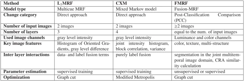
In the paper, we compare three state-of-the-art multilayer MRF techniques for change detection, which have been devel-oped for optical remote sensing image analysis. For a graphical comparison, Figs 1-3 show the structures and the processing workflows of the three models. The main properties of the dif-ferent techniques are summarized in Table 1.
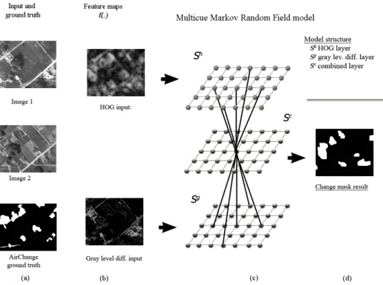
The Multicue MRF model (L3MRF, Fig. 1) (Singh et al.,
2014) integrates the modified Histogram of Oriented Gradients (HOG) and graylevel difference (GLD) features into the orig-inal Multi-MRF structure framework proposed by Kato et al. (2002), where two layers correspond to the two feature maps and the third one is the final segmentation layer. The class models and the inter-layer interaction terms are both affected by observation dependent and prior constraints, while within a given layer the prior Potts terms (Potts, 1952) ensure a smooth segmentation.
The second discussed method is theConditional Multilayer Mixed MRF(CXM, Fig. 2) proposed by Benedek and Szir´anyi (2009). CXM has - in a first view - a similar structure to the L3MRF, however, we can find a number of key diff
er-ences. First, CXM is a multilayer implementation of Mixed Markov models (Fridman, 2003), which uses besides regular MRF nodes the so called address nodes in the graph. Address nodes can link regular nodes in a flexible way based on vari-ous data- and prior conditions, ensuring a configurable graph structure. Second, in CXM the feature maps only affect di-rectly the individual graph nodes, while the interaction terms implement purely prior label fusion soft-constraints. Third, the applied features are also different from L3MRF. In CXM, the
change detection result is based on two weak features: global intensity co-occurrence statistics (ICS) and block correlation; while as a third feature, a contrast descriptor locally estimates the reliability of the weak change descriptors at each pixel po-sition.
Regarding the targeted application fields and the expected image inputs, the scopes of the L3MRF and CXM model are
quite similar. Both work on grayscale inputs and their output is a binary change mask. As practical differences, CXM may handle better scenarios when large radiometric differences may occur between unchanged regions, while L3MRF is quicker and
less sensitive to the presence of registration errors.
While the L3MRF and CXM models have a similar
struc-ture, the Fusion-MRF Model (FMRF, Fig. 3) proposed by Szir´anyi and Shadaydeh (2014) follows a significantly diff er-ent approach. First, while L3MRF and CXM aredirect
tech-niques working without any land cover class models, FMRF is a Post-Classification Comparison (PCC) method which simul-taneously implements an adaptive segmentation and change de-tection model for optical remote sensing images. Even the con-cept of layer is significantly different here. While in the first two models the different layers correspond to different image fea-tures, in FMRF each layer represents given input image; Thus ’multi-layers’ refers to multi-temporal images.
As another important difference between the models, FMRF has been designed to compare several images (two or more)
Method L3MRF CXM FMRF
Model type Multicue MRF Mixed Markov model Fusion-MRF
Change category Direct approach Direct approach Post-Classification Comparison (PCC)
Number of input images 2 images 2 images ≥2 images
Number of layers 3 4 equal to the num. of input images
Used image channels gray level intensity gray level intensity Luminance and color channels
Key image features Histogram of Oriented Gra-dients, gray level difference
joint intensity histogram, block correlation, variance
color, texture, multi-structure
Inter layer interactions data- and label fusion terms purely label fusion segmentation in the joint multitem-poral image domain, CRA similar-ity calculation
Parameter estimation supervised training supervised training unsupervised or supervised
Optimization Graph cut Modified Metropolis Graph cut
Table 1: Main properties of the discussed three models.
from different time instances, while the L3MRF and CXM
methods can compare always two multitemporal images. It is also possible to use the FMRF with an input of an image pair, but the use of three or more images are generally preferred to enhance cluster definitions depending on the quality of the im-ages and the degree of similarity between these imim-ages. The FMRF method applies clustering on a fused image series by us-ing the Cluster Reward Algorithm (CRA) (Inglada and Giros, 2004) as cross-layer similarity measure, followed by a multi-layer MRF segmentation (see Fig. 3). The resulted label map is applied for the automatic training of the single layers. After the segmentation of each single layer separately, changes are detected between the single label-maps.
Although the selected techniques have been mainly tested on optical images, no specific information of image sources is pre-scribed. However, since L3MRF and CXM are based on
sin-gle channel inputs, they typically expect intensity images pro-vided by airborne or spaceborne sensors. On the other hand, the FMRF method can deal with multi-modal as well as multispec-tral images. Here during the tests with FMRF, the chrominance (i.e. color) channels of the images are also exploited, while in the original paper (Szir´anyi and Shadaydeh, 2014), the Reader may also find an example for fusion with an infra-red image.
There are also differences in the applied MRF optimization techniques, which affect the quality and computational speed of the change detection process. Due to the sub-modular struc-tures of the L3MRF and FMRF models, the energy function can
be optimized by the efficient graph-cut based technique. On the other hand, the complex structure components of CXM yield that the energy optimization process is more complicated, and the computationally more expensive simulated annealing algo-rithm should be adopted.
As for the use of training data, L3MRF and CXM are
super-vised models, i.e. the feature model parameters are set using training regions. On the other hand, the FMRF model may be used both in an unsurpervised and in a supervised way upon the availability of manually labeled sample regions.
Regarding the necessary image resolution, our experiments showed that a minimum of 0.5m/pixel is expected, if we want to
highlight e.g. built-in changes in semi-urban areas. There is no explicit upper limit for the image resolution, since the focused techniques use pixel-level and block-based features, and the sizes of blocks can be upscaled for photos with larger resolution (some experiments with 1.5m resolution images were presented in (Benedek and Szir´anyi, 2009)). For the FMRF model, image resolution affects the accuracy of detected changes as discussed in Sec. 7.3.
Although the discussed three models are able to support var-ious applications, they also face some joint limitations. First, since the methods are purely based on pixel level or rectangular block-based image features, only very limited amount of ge-ometric object information can be incorporated in the models. Therefore at object level, geometric approaches such as Marked Point Processes (Benedek et al., 2012) could be used more efficiently. Secondly, since the outputs are binary change/no change masks, the techniques aredirectlynot suitable for high-lighting specific kinds of changes or novelty detection (such as distinguishing new and demolished buildings). However, there are someindirectoptions for change classification. Due to the nature of the PCC approach, if we train the supervised FMRF with semantically meaningful training classes (such as built-in vs. natural areas), we can provide a classification of the changes through the different class transitions. We can also cluster the changes in the CXM model in a limited way, by highlighting only the ICS based (homogeneous regions) or the correlation based (textured urban areas) differences.
3. Change Detection with the Multicue MRF Model
In Singh et al. (2014), aMulticue Markovian modelhas been proposed for change detection in registered optical aerial image pairs with large time differences. AMulticue Markov Random Fieldtakes into account information at two feature layers from two different sets of features:
• difference of a modified Histogram of Oriented Gradients (HOG) and
Figure 1: Structure of the L3MRF model and overview of the Multicue change detection process. Column (a): registered input images and ground truth change
mask for validation, Column (b): feature maps, Column (c): Structure diagram of the L3MRF model, Column (d): Output change mask
Figure 2: Structure of the CXM model and overview of the segmentation process. Column (a): inputs and and ground truth, Column (b):g(.),ν(.) andc(.) feature maps extracted from the input image pair. Column (c): Structure diagram of the CXM model. (note: the inter-layer connections are only shown regarding three selected pixels), Column (d): Output label maps of the four layers after MMD optimization. The segmentation result is obtained as the labeling of theS∗layer.
Figure 3: Structure of the FMRF model and workflow of the implementedPost-Classification Comparisonprocess.
The third layer provides the final change detection by a prob-abilistic combination of the two feature layers via MRF inter-actions. Thus we integrate both the texture level as well as the pixel level information to generate the final result. The pro-posed model uses pairwise interactions which also ensures that sub-modularity condition is satisfied. Hence a global energy optimum is achieved using a standard max-flow/min-cut algo-rithm ensuring homogeneity in the connected regions (Singh et al., 2014).
3.1. Image Model and Features
Let us consider a registered gray scale image pair, G1 and
G2, over the same pixel latticeS ={s1,s2...,sN}. We denote the
grayscale values of a given pixels∈S byg1(s) andg2(s) in the
first and second image, respectively. The goal is to classify each sites∈S as changed (foreground) or unchanged (background). Hence the assignment of a label to a particular site is from the set: λ = {fg,bg}where fg refers to foreground class and bg refers to the background class. The background/ foreground classes are modeled as random processes generating the ob-served image features. These random processes are modeled by fitting a suitable distribution function over the histograms cor-responding to each of the foreground and background classes using a set of training image pairs. The training image pairs contain a Ground Truth having all the pixels manually labeled by an expert. The features adopted in Singh et al. (2014) char-acterize the changes in terms of intensity (GL difference) and in terms of texture/structure (HOG difference).
The graylevel (GL) difference featured(s) computed over the
aligned image pairs for each corresponding pixel is simply d(s)=g1(s)−g2(s). (1)
Analysing the histogram of the background class using the WAFO toolbox (Brodtkorb et al., 2000), the generalized gamma density proved to be a good parametric model to represent these features, thus Pd(s)|bg= f(d(s)|a,b,c)= c bacΓ(a)d(s) ac−1e−d(bs) c , (2) where Γ(.) is the gamma function, and (a,b,c) are the back-ground parameters.
As for the foreground, basically anyd(s) value is allowed, hence it is represented by a uniform density function given as
Pd(s)|fg=⎧⎪⎪⎨⎪⎪⎩
1
bd−ad, ifd(s)∈[ad,bd].
0, otherwise. (3)
using (ad,bd) foreground parameters.
The Histogram of Oriented Gradient (HOG) is a feature de-scriptor that has mainly been used for object detection. It ba-sically involves counting the number of occurrences of diff er-ent orier-entations of gradier-ents inside fixed sized windows and then rounding it to the correct bin of the histogram. In Dalal and Triggs (2005) the image was divided into blocks and then further into small cells for which the histogram of gradients is computed. Finally the concatenation of all resulting histograms leads to the descriptor for the entire image. The HOG feature used in Singh et al. (2014) is a somewhat modified version of
the original method proposed in Dalal and Triggs (2005): in-stead of cells, a sliding window of size 11×11 is used to com-pute HOG. Given the gradients (Ix,Iy) computed at each pixel
via a standard finite difference operator, the magnitude and ori-entation can be calculated using the following equations:
H= I2 x+Iy2 θ=arctan Iy Ix
Note thatθ ∈ [0, π/2]. Then a HOG with9 binsis computed at every position of the sliding window over the entire image, yielding a 9 dimensional vector→−fs associated with every pixel
s ∈ S. The HOG difference featureh(s) corresponding to a particular pixelsis thus given by:
h(s)=−→fs1− −→
fs2 (4)
As for the GL difference feature, the background is mod-eled as a generalized gamma density function Ph(s)|bg = f(h(s)|u,v,w) with parametersu,v,wand the foreground is rep-resented as a uniform distribution over the [ah,bh] interval.
3.2. Multicue Model
Using the featuresd(s) andh(s), a three-layer MRF model is constructed in Singh et al. (2014) to solve the change detection problem as a foreground/background segmentation. As shown in Fig. 1, the proposed MRF segmentation model (Kato et al., 2002; Kato and Zerubia, 2012) is built over a GraphG com-posed of three different layers, namelySh,ScandSg, all being
of the same size as the latticeS of the input images. Each pixel s ∈ S has a corresponding site associated with it in each of these layers denoted as
sh∈Sh, sc∈Sc, sg∈Sg (5)
where Sh,ScandSg are the layers representing the modified
HOG difference feature, final desired change map, and GL dif-ference feature respectively.
Every sitesi,i ∈ {h,c,g}has also a class label associated to
it, which is denoted byω(si) and modeled as a discrete random
variable taking values from the label setλ={fg,bg}. The hid-den label process is thus the set of all the labels over the entire graphGas follows:
ω=ω(si)|s∈S,i∈ {h,c,g} (6) The neighborhood system (representing the conditional depen-dencies of nearby sites) are shown in Fig. 1. The intra-layer interactions consist ofsingletonanddoubletoncliques denoted byC1andC2, respectively. These cliques correspond to a stan-dard first order neighborhood system (Kato and Zerubia, 2012), in whichsingletons with single individual sites are linking the model to the two observation features, whiledoubletons ensure homogeneity within each layer. Note thatsingletons are not de-fined for the combined layerScas it has no direct interaction
with the observations, while for the other two layers, single-tons represent the HOG features forShand GL features forSg,
yielding the observation process
F ={h(sh)|s∈S} ∪ {d(sg)|s∈S}, (7) The inter-layer cliques, marked byC5, are doubletons as dis-played in Fig. 1, and they are responsible for feature integration. Hence the graphGhas the set of cliques
C=C1∪ C2∪ C5 (8)
The goal is to find the optimal labelingωwhich maximizes the a posteriori probability P(ω|F), which is the maximum a posteriori (MAP) estimate (Geman and Geman, 1984) given as
ω=argmax
ω∈Ω P(ω|F) (9)
whereΩdenotes the set of all the possible labellings. Based on the Hammersley-Clifford theorem, the posterior probability for a particular labeling follows a Gibbs distribution:
P(ω|F)= exp(−U(ω)) Z = 1 Zexp ⎛ ⎜⎜⎜⎜⎜ ⎜⎝− C∈C VC(ωC) ⎞ ⎟⎟⎟⎟⎟ ⎟⎠ (10)
whereU(ω) is the energy function, VC denotes theclique
po-tentialof a cliqueC ∈ Chaving the label configuration ωC, andZ is a normalization constant independent of ωgiven by Z = ω∈Ωexp(−U(ω)). Therefore by defining the potentials VCfor the cliques completes the MRF model definition and the
above MAP problem becomes a standard energy minimization problem.
Since the labellings forSh andSg layers are directly
influ-enced by the values ofh(.) andd(.) respectively,∀s ∈ S the singleton will link these layers to the respective observations as:
V{sh}(ω(sh)) = −logP(h(s)|ω(sh)) (11)
V{sg}(ω(sg)) = −logP(d(s)|ω(sg)), (12)
where the conditional probabilitiesP(.|ω(.)) given that the la-bel being a background or a foreground class generate theh(s) ord(s) observations, has already been defined in Section 3.1. However, the labels corresponding to the sites of theSclayer
have no direct influence by these observations and hence the singleton cliques onScare not used.
For the intra-layer cliquesC2 ={si,ri}whereC2 ∈ C2 and
i∈ {h,c,g}, a simple Ising-type potential (Besag, 1986) can be used to ensure local label homogeneity:
VC2
ω(si), ω(ri)=⎧⎪⎪⎨⎪⎪⎩0, ifω(s
i)=ω(ri).
2Ki, ifω(si)ω(ri). (13)
wherei∈ {h,c,g}.Ki≥0 is a parameter controlling the homo-geneity of the regions. AsKiincreases, the resulting regions
in the corresponding layer (indexedi) become more homoge-neous.
C5and{i,j} ∈ {{h,c},{c,g}}, and the potentials are given by: VC5 = f ω(si), ω(rj)= ⎧⎪⎪ ⎨ ⎪⎪⎩ρ hc∗W r∗ V{sh}(ω(sh))−V{sh}(ω(rh)), (a). ρcg∗W r∗ V{sg}(ω(sg))−V{sg}(ω(rg)), (b). (14) where (a) and (b) refer to{i,j} = {h,c}and{i,j} = {c,g} re-spectively. AlsoV{sh}(ω(.)) andV{sg}(ω(.)) are the singleton
po-tentials for the sites sh ∈ Sh and sg ∈ Sg dependent on the
labelingω(.). Both parameters (ρhc ≥0 andρcg ≥0) control
the influence of the feature layers(ShandSg) to the combined
(Sc) layer. W
ris the weight of the interaction. Higher weight
(Wr=0.6) is assigned to the corresponding site whereas smaller
weights (Wr=0.1 each) to the other 4 neighboring sites.
Hence the optimal MAP labeling ω, which maximizes P(ω|F) can be calculated as the minimum energy configuration (Singh et al., 2014) ω=argmin ω∈Ω − s∈S logP(h(s)|ω(sh))− s∈S logP(d(s)|ω(sg))+ C2∈C2 VC2(ωC2)+ C5∈C5 VC5(ωC5) (15)
4. Change detection with the Multilayer Conditional Mixed Markov Model
In Benedek and Szir´anyi (2009), a Multilayer Conditional Mixed Markov model (CXM) has been proposed for change de-tection in optical image pairs. The CXM is defined as the com-bination of a mixed Markov model (Fridman, 2003) and a con-ditionally independent random field of signals. The model has four layers: three of them are feature layers, while the fourth one is the final segmentation layer, having a similar role to the combined layer of the L3MRF model. The feature layers
corre-spond to the following descriptors:
• joint 2D gray level histogram of the multitemporal image inputs
• normalized block correlation using a fix sized window around each pixel
• variance of gray levels within a sliding window for local contrast estimation
Since the gray level histogram and the correlation are comple-mentary features working either in homogeneous or in highly textured image region, the variance descriptor plays an indica-tor role: Based on the local contrast, one can decide which fea-ture is more reliable at a given pixel location. The fourth layer provides the final change detection by a probabilistic combina-tion of the three feature layers via MRF interaccombina-tions. Similarly to L3MRF, pairwise interactions are used between the nodes,
but as a significant difference, the variance layer is composed of address nodes of the Mixed Markov model, while all the other layers contain regular nodes.
4.1. Image model and features
Here the same image model and the corresponding notations are used as introduced in Sec. 3.1 by the L3MRF model. The
starting step of the modeling process is again the extraction oflocal featuresat each s ∈ S which give us information for classifyingsas a changedforeground(fg) or unchanged back-ground (bg) surface point. The fg/bg classes as considered henceforward as random processes generating the features ac-cording to different distributions.
Thefirst featurein the CXM model is based on the investi-gations in the joint intensity domain of the two images. Here, instead of prescribing an intensity offset or other global linear transform between the correspondingg1(s) andg2(s) gray
lev-els (as seen by the L3MRF), we give a multi modal description
of the observed data. We approximate the 2-D histogram of the g(s) = [g1(s),g2(s)]T vectors by a mixture of Gaussians
dis-tribution. In this way, one can measure which intensity values occur often together in the two images. Thereafter, the prob-ability of theg(s) observation in the background is calculated as: Pg(s)bg = Ki=1κi·ηg(s), μi,Σi,where η(.) denotes a
two dimensional Gaussian density function withμi mean vec-tor and Σi covariance matrix, while the κi terms are positive
weighting factors. Using a fixedK = 5, the distribution pa-rameters are estimated automatically by the conventional EM algorithm. On the other hand, anyg(s) value may occur in the changed regions, hence the ‘ch’ class is modeled by a uniform density:Pg(s)fg=u. However, this multi-Gaussian intensity based approach (MGI) may erroneously mark several unaltered regions as changes compared: the miss-classifications would mainly be limited to highly textured regions (e.g. buildings and roads) since theg(s) gray values occurring there are less fre-quent in the global image statistics.
For obtaining thesecondfeature, denoted byc(s), we calcu-late the correlation between the rectangularz×zneighborhoods of sinG1 and inG2 (usedv = 17). Pixels with higherc(s)
values lie more likely in unchanged image regions. The exper-iments of the authors showed that theP(c(s)|bg) andP(c(s)|fg) probabilities can be approximated by different Gaussian dis-tributions. Note that in itself, a simple Maximum Likelihood (ML) classification based onc(.) would also results in a fairly poor segmentation, but theg(s) andc(s) are efficient comple-mentary features. In low contrasted image regions, where the noisyc(s) may be irrelevant, the decision based ong(s) is reli-able. In textured areas one should choosec(s) instead ofg(s).
As the previous paragraphs suggest, we may estimate the re-liability of the segmentation based on theg(s) intensity respec-tivelyc(s) correlation features at each pixels. Letνi(s) be the
variance of the gray levels in the neighborhood of s, and let beν(s)=[ν1(s), ν2(s)]T. For implementing a probabilistic
fea-ture selection process, we approximate theν(s) variances of the lowandhighcontrasted image regions by 2-D Gaussian density functions, where the parameters are estimated with an iterative algorithm presented in Benedek and Szir´anyi (2009).
4.2. Multilayer Mixed Markov model
As mentioned in the introduction, Mixed Markov models (Fridman, 2003) extend the modeling capabilities of Markov
random fields: they enable using both static and observation-dependent dynamic links between the processing nodes. We can take here the advantage of this property, since theν(s) fea-ture plays a particular role: it may locally switch ON and OFF the g(s) and c(s) features into the integration procedure. We consider the task as a composition of four interactive segmenta-tion processes. Thus we project the problem to a graphGwith four layers: Sg,Sc,SνandS∗. We assign to each pixel s∈S a unique graph node in each layer: e.g. sg is the node corre-sponding to pixel son the layerSg. Denote sc ∈ Sc,sν ∈ Sν
ands∗∈S∗similarly.
Following the approach of Sec. 3.2, we introduce next the la-beling random process, which assigns a labelω(.) to all nodes of
G. As usual, graph edges express direct dependencies between the corresponding node labels. The present approach exploits that Mixed Markov models distinguish two types of processing units, calledregularandaddressnodes (Fridman, 2003). The Sg,Sc, andS∗layers containregular nodes, where the label
de-notes a possible fg/bg segmentation class:∀s∈S,i∈ {g,c,∗}: ω(si) ∈ {fg,bg}.For each s,ω(sg) resp. ω(sc) corresponds to
the segmentation based on theg(s) resp.c(s) feature; while the labels at theS∗layer present the final change mask.
On the other hand, the Sν layer contains address nodes, where forsν∈Sνthe labelω(sν) is a pointer to a regular node of G. In contrast with static edges, address pointers represent dynamic connections between the nodes.
We use the following notations: ˜ω(sν) := ω(ω(sν)) is the label of the (regular) node addressed bysν, andω={ω(si)|s∈
S, i∈ {g,c, ν,∗}}denotes a global labeling. LetF ={Fs|s∈S}
be the global observation, where Fs is the union of theg(s),
ν(s) andc(s) local features extracted at pixel s. By definition of Mixed Markov models (Fridman, 2003), (static) edges may link any two nodes, and the a posteriori probability of a given global labelingωis given by:
P(ω|F)=α
C∈C
exp−VC
ωC, ωνC,F , (16)
whereCis the set of cliques inG. ForC ∈ C:ωC ={ω(q)|q ∈
C}andωνC={ω˜(sν)sν∈Sν∩C}.VCis aC →Rclique
poten-tial function, which has a ‘low’ value if the labels within the set ωC∪ωνCare semantically consistent, whileVC is ‘high’
other-wise. Scalarαis a normalizing constant, which is independent ofω. Note that we will also usesingleton cliqueswhich contain single nodes.
Next, we define the cliques ofGand the correspondingVC
clique potential functions. The observations affect the model through the singleton potentials. As we stated previously, the labels in the Sg and Sc layers are directly influenced by the
g(.) respectively c(.) values, while the labels in S∗ have no direct links with these measurements. For this reason, let be V{sg} = −logPg(s)ω(sg), V{sc} = −logPc(s)ω(sc) and
V{s∗} ≡ 0. Note that the above distributions were already
de-fined in Section 4.1, andV{sν}will be later given.
For presenting smooth segmentations, we put connections within each layer among node pairs corresponding to neighbor-ing pixels on theS image lattice. Denote the set of the resulting
intra-layercliques byC2. The prescribed potential function of a clique inC2will penalize neighbouring nodes having diff er-ent labels. Assumingr ands to be neighboring pixels onS, the potential of the doubleton cliqueC2={ri,si} ∈ C2for each
i∈ {g,c, ν,∗}is calculated similarly to formula (13) from Sec. 3.2.
We continue with the description of theinter-layer interac-tions. Based on previous investigations,ω(s∗) should mostly be equal either toω(sg) or toω(sc), depending on the observed
ν(s) feature. Hence, we put an edge amongs∗andsν, and pre-scribe that sν should point either to sg or to sc . As for the
singleton potentials in theSνlayer, ifsνpoints tosψ|ψ∈{g,c}, let beV{sν} =−logPν(s)hψ. On the other hand, we get the po-tential of theinter-layer clique C3 ={s∗,sν}with a fixedρ >0
as VC3 ω(s∗),ω(˜ sν)= 0 if ω(s∗)=ω˜(sν) ρ otherwise
Finally, based on (16), theωmaximum a posteriori estimate of the optimal global labeling, which maximizesP(ω|F) (hence minimizes−logP(ω|F)) can be obtained as:
ω=argmin ω∈Ω s∈S;i V{si}ω(si),Fs+ + {s,r}∈C2;i VC2 ω( si), ω(ri)+ s∈S VC3 ω( s∗),ω(˜ sν) (17) wherei ∈ {g,c, ν,∗}andΩdenotes the set of all the possible global labelings. The final segmentation is taken as the labeling of theS∗layer.
5. Multitemporal Image Segmentation with the Fusion-MRF Model
In the Fusion-MRF (FMRF) method (Szir´anyi and Shaday-deh, 2014), remote sensing areas of fused image series are ex-amined in different levels of MRF segmentation; the goal is to automatically detect the category changes of the yearly trans-muting areas having rich variations within a category by using more sample layers. The overlapping combination of category variations can be collected in a multilayer MRF segmentation; this supports the layer-by-layer MRF segmentation and change detection later. The definition of change is parallel to the def-inition of similarity; locations of image time series data that come from different sensors at different lighting and weather conditions can be compared if robust in-layer and cross-layer descriptors could be found. For this reason, in the proposed FMRF method, block-wise similarity measures is added to the stacking of the layers’ pixel/microstructure information; the au-thors propose to use Cluster Reward Algorithm (CRA) (Inglada and Giros, 2004) in the multilayer fusion calculated between layer pairs in the series. The novelties of the FMRF approach are discussed in the following:
• Finding clusters on the stack of image-layers results in aligned cluster-definitionfor the different layers;
• Fused segmentation on the stack of image-layers, resulting inmultilayer labeling;
• Multilayer labeling is used for theunsupervisedclustering of the single-layer labeling; this aligned labeling makes thechange detection unequivocal;
• A noise-tolerant cross-layer similarity measure,CRA, is used to better identify some classes where radiometric val-ues are dubious.
5.1. Multitemporal Image Model and Similarity Feature In a series of N layers of remote sensing images, let xLis denote the feature vector at pixel s of layer Li,
i = 1,2,· · ·,N. This feature vector might contain color, texture/micro-structural features, cross layer similarity mea-sures, or mixture of these. SetX ={xs|s∈S}marks the global
image data. An example of a feature vector would be
xLis =[xCLi(s),xLiM(s)]T (18) where xCLi(s) contains the pixel’s color values, andxLiM(s) is the cross layer similarity measures between the image and other two or more images in the series. The cross layer similarity measure might be correlation, mutual information, orCRA.
The multiple layers of remotely sensed images time series are characterized by the stack xLi1...in
s of these vectors for a
rea-sonable set of them,n≤N: xLi1...in s ={x Li1 s ,x Li2 s , ...x Lin s } (19)
Different similarity measures have been considered in the preliminary tests, such as distance to independence, mutual in-formation, CRA (Inglada and Giros, 2004), Kullback Leibler divergence (see (Alberga, 2009) and references therein). The CRAsimilarity measure is chosen as it gives better segmenta-tion and change detecsegmenta-tion results than other similarity measures such as Kullback Leibler divergence and mutual information. 5.2. Fusion-MRF: multilayer segmentation and change
detec-tion
The segmentation and change detection procedure contains different levels of MRF optimization in the following main steps:
1. Selecting and registering the image layers; an example is shown in Inglada and Giros (2004). In case of professional data suppliers orthonormed and geographically registered images are given; no further registration is needed. In the discussed method no color-constancy or any shape/color semantic information is needed; the color of the corre-sponding areas and the texture can differ strongly layer-by-layer.
2. Finding clusters in the set of vectors (xLi1...in
s ) and
calcu-lating the cluster parameters (mean and covariance of the conditional term in (22)) for the fusion based ”multilayer clusters”. This step can be performed either by using un-supervised methods such as the K-means algorithm, or by choosing the characteristic training areas manually.
3. Running MRF segmentation on the fused layer data (xLi1...in
s ) containing the cross-layer measures, and the
multi-layer cluster parameters, resulting in a multimulti-layer labeling
ΩLi1...in;
4. Single-layer training: the map of multilayer labeling
ΩLi1...in is used as a training map for each image layerLi:
cluster parameters are calculated for each single layer con-trolled by the label map of multilayer clusters.
5. For each single layer Li (containing only its color and
maybe texture features) a MRF segmentation is processed, resulting in a labeling:ΩLi;
6. The consecutive image layers (...,(i−1),(i), ...) are com-pared to find the changes among the different label maps to get theδi−1,ichange map:
δi−1,i(.)=
ΩLi(.)ΩLi−1(.)
=TRUE (20) In the proposed segmentation algorithm a multilayer MRF model is applied by contributing the term of the cross-layer CRAsimilarity measure calculated between each pair in a sub-set of three or more consecutive images. In what follows three consecutive images are used, however the algorithm can be eas-ily extended to more layers. The stack of feature vectorsxL1...3
s
is generated as follows
1. For each pair of the three consecutive imagesLi,Li+1 and
Li+2, theCRAimage is calculated. In the calculation of the
CRAimage at each pixel, we useD×D-pixel estimation window around this pixel to calculate the local histograms; Let the obtained CRA images beCRA(i,i+1),CRA(i+1,i+ 2), andCRA(i,i+2).
2. LetxLis denote the luminance value of pixelsin imageLi.
Construct the stack of feature vectors for pixels sin the three imagesLi,Li+1andLi+2as follows:
xLi,i+1,i+2 s = [xLis +αCRAs(i,i+1), xLi+1 s +αCRAs(i+1,i+2), xLi+2 s +αCRAs(i,i+2)]T (21)
whereαis a positive normalizing scalar ensuring the same range of the two different terms.
Note that the use of the addition ofxLis andCRAs(i,i+1) in
the feature vector as given in (21) means lower dimensional-ity than using these features as two separate values as in (18). However, with the assumption thatxLis andCRAs(i,i+1) are
statistically independent, it can be verified that they will con-tribute similar terms to the energy of MRF as when they are used as two separate features.
Next, we define the MRF energy model. Let S =
{s1,s2, ...sH} denote the image pixels, and ω = {ω =
(ωs1, . . . , ωsH) : ωsi ∈ Λ,1 ≤ i ≤ H}be the set of all
The output labeling is taken again as the MAP estimator of the following energy function:
ω=argmin ω∈Ω s∈S −logP(xs|ω(s))+ r,s∈S VC2(ω(r), ω(s)) (22) where similarly to the intra-layer interactions in the L3MRF and
CXM methods, the Potts constraint (Potts, 1952) is used again to obtain smooth connected regions in the segmentation map (see formula (13) from Sec. 3.2).
6. MRF optimization
There is a large variety of MRF optimization algorithms used by the different change detection models, such as the Iterated Conditional Modes (ICM) (Besag, 1986) algorithm, or various simulated annealing techniques. Graph cut based minimiza-tion techniques have particularly become popular in the last ten years, since unlike the above iterative approaches, they guar-antee to provide the global minimum of the energy in polyno-mial time. However the energy function must fulfill a number of specific requirements which must be considered during the modeling phase, limiting the possible model structures.
The Multicue MRF segmentation model presented in Sec-tion 3.2 provides a binary labeling, where a labelω(si),s ∈S
and i ∈ {h,c,g}, can be regarded as a binary variable taking values 0 and 1. Moreover, the Gibbs energy given in (15) is composed of singleton and doubleton potentials only, i.e. the model has unary and pairwise interactions only. Therefore the Gibbs energy in (15) can be represented as a weighted graph
G = (V,E) (Kolmogorov and Zabih, 2004). The set of ver-tices’s Vin the graph Gconsists of all the sites of the three-layer MRF model and two terminal nodes: the source sand the sink t. The edgesE are present between interacting sites as defined by the MRF model and special edges are connect-ing each site with the terminal nodessandt(for more details see (Kolmogorov and Zabih, 2004)). Estimating the minimal energy configuration is equivalent to compute the min cut/max flow on the corresponding graphG. The energy functionE(ω) is composed of unary and pairwise interactions (Kolmogorov and Zabih, 2004): E(ω)= s∈S Es(ω(si))+ (s,r)∈C−{C1} Es,r(ω(si), ω(rj)) (23)
where i,j ∈ {h,c,g}; i = j for intra-layer cliques and inter-layer clique’s otherwise. The above equivalence between en-ergy minimization ofEand the min cut/max flow on the graph is only true, if E also satisfies the submodularity constraint. Hence the authors used a standard graph-cut algorithm imple-mented by Vladimir Kolmogorov (http://pub.ist.ac.at/
~vnk/software.html) to minimize the energy in (15). The energy term of (16) in the CXM model can be minimized by conventional iterative techniques, like ICM or simulated an-nealing (Geman and Geman, 1984). For choosing a good com-promise between the quality factor and processing speed, the
CXM model adapted the deterministic Modified Metropolis re-laxation algorithm (Kato and Zerubia, 2012) to the multilayer model structure, as detailed in Benedek and Szir´anyi (2009). Accordingly the four layers of the model are optimized simul-taneously, and their interactions develop the final segmentation, which is taken at the end as the labeling of theS∗layer. As the authors noted, due to the fully modular structure of the en-ergy term, the introduced model could be completed straight-forwardly with additional sensor information (e.g. color or infrared sensors) or task-specific features depending on avail-ability, in exchange that the iterative optimization takes usually longer time than the graph-cut optimization.
Similarly to the L3MRF model, the FMRF energy function
can be optimized by graph cut based techniques. The authors in Szir´anyi and Shadaydeh (2014) adopted theα-expansion algo-rithm for MRF energy minimization, using the implementation of Szeliski et al. (2006). This relaxation technique ensures the convergence to a solution, where the energy is guaranteed to be under a boundary defined by the global minimal solution mul-tiplied by a constant factor.
7. Parameter settings in the different model
The L3MRF and CXM models follow asupervisedapproach
of change detection. Hence all the parameters are estimated us-ing the trainus-ing data provided in each of the three data sets. Regarding the data term parameters, different feature distri-butions for the changed and unchanged regions should be es-timated based on the empirical feature histograms obtained from the labeled training data. The standard Expectation-Maximization (EM) algorithm was applied in both models, however in CXM the EM steps were embedded into an itera-tive framework due mutual dependency between the parameters (Benedek and Szir´anyi, 2009).
In the FMRF, calculation of the cluster parameters for the fusion based multilayer clusters can be performed either by us-ing unsupervised methods such as the K-means algorithm, or by supervised training by choosing the characteristic training areas manually. In all experiments presented here the unsuper-vised K-means algorithm was used.
7.1. L3MRF parameters
The following parameters are used in the proposed model which need to be estimated :
• Parameters for Modified HOG feature selection:{dw,nb}
• Parameters of the various pdf’s as introduced in (3), (4), (6), (7) :{a,b,c,u,v,w,ad,bd,ah,bh}
• Parameters of the intra-layer and inter-layer clique poten-tial functions :{Ki, ρhc, ρcg}wherei∈ {h,c,g}
The initial parameters for the HOG feature selection namely the detection window sizedwand the bin sizenbwere set by evalu-ating the maximum-likelihood results. By experimentation the desired results were obtained by setting the detection window to 11×11 and the number of bins to 9 (Singh et al., 2014).
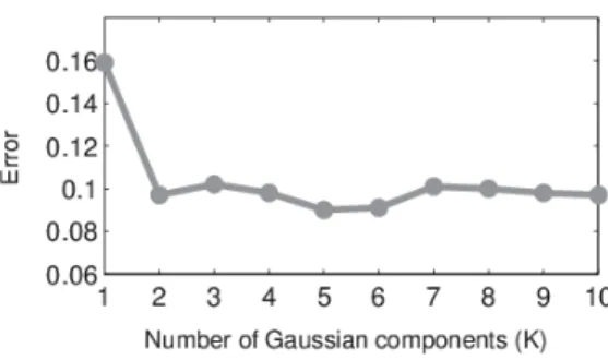
Figure 4: CXM parameter analysis example. Error of the mixture of Gaussians approximation of the joint intensity statistics as a function of the number of mixture components (K).
Parameters for the Generalized Gamma Distribution (in (3), (6)) corresponding to the background class (both for the gray level and the Modified HOG features) were learned from the training data provided in each of the data sets. The threshold values for the uniform distribution (in (4), (7)) corresponding to the foreground class for both the gray level and the HOG features were set to the optimal values again for each of the training data belonging to its respective data set.
The intra- and inter-layer clique potentials are independent of the input images hence we set their values by trial and error over a small training dataset and then keep these values for all input image pairs.
7.2. CXM parameters
The CXM segmentation model has the following parameters:
• Preliminary parameters of feature calculation (see Sec. 4.1):Λ ={K,z}
• Parameters of the probability density functions introduced in Sec. 4.1:Θ ={μi,Σi|i∈1. . .K} ∪ {μc, σc, μψ,Σψ}
• Parameters of the intra- and inter-layer potential functions:
Φ = ρ,Ki:i∈ {g,c,∗, ν}!
The first step is determining the Λpreliminary parameters. K, which is the number of the Gaussian mixture components in the background’s intensity model, was set by a quantitative analysis. We considered the distribution sequencePK(g(s)|bg)
for K =1,2, . . .wherePK is obtained by EM estimation from
the training data using K mixture components. Thereafter we measured the Bhattacharyya distances between the empir-ical histogram and the approximated distributions. As Fig. 4 demonstrates in the Szadaset, the minimal error has been
ob-served at K = 5, but the variance of the measured error rates was under 10% for the differentKcomponents between 2 and 10.
On the other hand the size of the correlation window z particularly depends on the image resolution and textureness. Since in the considered images the buildings were the princi-pal sources of texture, we have chosen a correlation window which narrowly covers an average house (for the three test sets
we usedz = 17). During the tests we found this choice op-timal: with significantly larger windows (z > 30) some indi-vidual building changes have been erroneously ignored, while small rectangles (z<5) reported many false changes.
After fixingΛ, theΘparameters can be obtained automati-cally from the training image pairs using conventional estima-tors embedded in an iterative framework as detailed in Benedek and Szir´anyi (2009). As for theΦparameter set, the experi-ments indicated that the model is not sensitive to a particular setting within a wide range, and these parameters can be esti-mated a priori. We usedρ=Ki=1,i∈ {g,c,∗, ν}.
7.3. FMRF parameters
The following parameters are used in the FMRF model
• Number of image layersNand number of classesH.
• Window sizeDused in the calculation of the CRA simi-larity measure.
• The homogeneity weightK used in the Potts term of the energy function.
For the present experiments using three image layers in the comparison gives good results. Using more layers requires di-mensionality reduction or larger training areas that assure the presence of sufficient independent samples. Moreover, in such case, the number of possible CRA image combinations is larger than the number of layers. The used CRA images can be se-lected on the basis of maximal cross-layer information com-plexity. The number of classes used is based on the change detection application.
In CRA similarity measure calculation, the choice of the win-dow size D, used in the estimation of local histograms, is se-lected based on the resolution of the images and the scale of the desired change detection. The size of the window should be less than the size of the change to be detected. The detection of small changes requires small window size; however larger window size gives better estimation of the CRA similarity mea-sures. In our experiments, a minimum window size of 5x5 win-dow is required regardless of image resolution to obtain good estimate of the local histograms used in CRA similarity mea-sure calculation. Finding the optimum window size for each point adaptively, along with the definition of the scale of change detection and the image resolution, needs further research. In an attempt to deal with this problem Shadaydeh and Szir´anyi (2014) proposed new method for improved similarity measure estimation using weighted local histograms. The weight as-signed to each pixel in the histogram estimation window fol-lows an exponential function of its distance from the center of the window and the corresponding pixel value in an initial change map image which is derived from other microstructure or radiometric information. This improved similarity measure benefits from the good detection ability of small estimation window and the good estimation accuracy of large estimation window; hence it can replace the time-consuming multi-scale selection approaches for statistics based similarity measures in remote sensing.
The homogeneity weightKwas again set by trial and error, similarly to the L3MRF model.
8. Method comparison
8.1. Test Databases and Experimental Conditions
For comparative evaluation of the L3MRF, CXM and FMRF
techniques, we used mainly the SZTAKI AirChange Bench-mark Set1. This benchmark has already been used in Benedek
and Szir´anyi (2009) for an extensive validation of the CXM model, which was compared to the then-state-of-the-art, and it serves well the comparison between CXM and L3MRF. The
benchmark contains images from three data sets of optical aerial images provided by the Hungarian Institute of Geodesy Cartography & Remote Sensing (F ¨OMI) and Google Earth and corresponding Ground Truth change masks. All the images have been aligned as orthophotos.
Thefirstdata set – called Szada– contains co-registered
im-ages taken by F ¨OMI in years 2000 and 2005. This test set con-sists ofseven- also manually evaluated - image pairs, covering in aggregate 9.5km2 area at 1.5m/pixelresolution (the size of
each image in the test set is 952×640 pixels). The second test set – called Tiszadob– includesfiveimage pairs from 2000
and 2007 (6.8km2) with similar size and quality parameters to Szada. Images of 2000 and 2005 were scanned on photo-films
(Hasselblad 500 EL/M) before digital scan. The 2007 image has been originally scanned in digital form (Nikon D3X, with AF-S Nikkor 50 mm 1.4G lens). Finally, in thethird data set– called Archive– an aerial image taken by F ¨OMI in 1984 can be
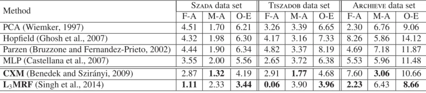
compared to a corresponding Google Earth image from around 2007. The latter case is highly challenging, since the image from 1984 has a degraded quality, and several major diff er-ences appear due to the 23 years time difference between the two shots. An important additional information is that the im-age pair from the Archiveset has been taken from the same area
as the first image pair of the Szadaset, therefore in this region
four co-registered images available with different time stamps (three of them are partially shown in Fig. 6). The latter fact can be utilized by the Fusion-MRF (FMRF) model (Szir´anyi and Shadaydeh, 2014), which may consider several images to obtain a robust change mask between two selected time layers. Considering the above conditions, during the experiments with the FMRF model, three image layers were used on the Szadadata set by extracting changes between years 2000 and
2005. The authors used as third (auxiliary) image the Google Earth photo of Archivefrom 2007. As the input of the PCC
ap-proach, two segmentation classes were used: one for urban and one for non-urban areas. The feature vector used for the mul-tilayer segmentation contained luminance value and the CRA similarity measure as defined in (21), while the CIE L*a*b* color values were only used in the single layer segmentation step. For change detection between years 1984 and 2007 (ex-periment Archive), the Szada2005 image was used as third
1http://web.eee.sztaki.hu/remotesensing/airchange_
benchmark.html.
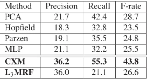
Method Precision Recall F-rate
PCA 21.7 42.4 28.7 Hopfield 18.3 32.8 23.5 Parzen 19.1 35.5 24.8 MLP 21.1 32.2 25.5 CXM 36.2 55.3 43.8 L3MRF 36.0 21.1 26.6
Table 3: Method evaluation:Precision,RecallandF-measurerates in percent w.r.t. the ‘change’ class in the Szadaset (higher values are preferred)
image. Similarly to the previous case, urban and non-urban regions have been distinguished during the segmentation and the used feature vector included luminance and CRA similar-ity. For single layer segmentation, luminance values and tex-ture featex-tures (output energy of Laws filters) were exploited. All the used features were normalized to have maximum value of 1. Finally athirdexperiment has been conducted in a fully natural (non-urban) region, called Forest(see Fig. 7), which was not
included in the AirChange Benchmark. From the selected area, three high resolution images (around 0.5m/pixel) were avail-able, but only two images were used in the final validation test, as the experiments did not report further improvement by in-cluding the third image. For the segmentation, three classes were defined here: meadow, planted meadow and forest. The feature vector contained the luminance and CRA similarity as usual. In single layer segmentation, no color components were used except luminance in addition to theLawsfeatures. 8.2. Ground Truth generation
Relevant Ground Truth (GT) generation is a difficult and of-ten controversial issue in change detection evaluation. For this reason, we will discuss two different GT approaches in this pa-per: one forDirecttechniques, and one forPost-Classification Comparison (PCC)methods, with also showing experiments for cross-validation.
InDirect methodsthe users often define from the application point of view the relevant types of changes, and they directly la-bel the changed regions. The creators of theAirChange Bench-mark Set followed this approach, and they considered three main prototypes of changes, as displayed in Fig. 5: (a) new built-up regions and building operations (b) planting of large group of trees of forestation (c) fresh plough-land or ground-works before building over. Note that this AirChange GT does NOT contain change classification, only binary changed-unchanged decision for each pixel.
On the other hand, inPCC methods, where the results of dif-ferent image segmentations are compared, the GT should be generated for the classification step at each time layer, there-after the change GT can be automatically derived as taking the image regions with altered class labels. This evaluation ap-proach is followed in theRegion PCC GTgeneration process of Szir´anyi and Shadaydeh (2014), where different segmentation classes have been considered for the different image pairs (see Sec. 8.1), such as urban and non-urban for Szadaand Archive;