Parametric bootstrap mean squared error of a small area multivariate EBLUP

Moretti, A

and

Shlomo, N

and

Sakshaug, JW

(2018)Parametric bootstrap

mean squared error of a small area multivariate EBLUP. Communications in

Statistics: Simulation and Computation. ISSN 0361-0918

Downloaded from:

http://e-space.mmu.ac.uk/625178/

Version:

Accepted Version

Publisher:

Taylor & Francis

DOI:

https://doi.org/10.1080/03610918.2018.1498889

Please cite the published version

1

Parametric Bootstrap Mean Squared Error of a Small Area Multivariate EBLUP

Angelo Moretti1_{, Natalie Shlomo}2 _{and Joseph W. Sakshaug}3

1 (Corresponding author). University of Sheffield, Department of Geography. Email:

[email protected] or [email protected]

2 University of Manchester, Social Statistics Department. Email:

[email protected]

2

Parametric Bootstrap Mean Squared Error of a Small Area Multivariate EBLUP

Manuscript

Abstract

This article deals with mean squared error (MSE) estimation of a multivariate empirical best linear unbiased predictor (MEBLUP) under the unit-level multivariate nested-errors regression model for small area estimation via parametric bootstrap. A simulation study is designed to evaluate the performance of our algorithm and compare it with the univariate case bootstrap MSE which has been shown to be consistent to the true MSE. The simulation shows that, in line with the literature, MEBLUP provides unbiased estimates with lower MSE than EBLUP. We also provide a short empirical analysis based on real data collected from the U.S. Department of Agriculture.

Keywords: Multivariate empirical best linear unbiased predictor; Model-based inference; Multivariate small area estimation; Multivariate multilevel models; Resampling

3

1. Introduction

Regional policies need to base their funding allocation on reliable statistical information. However, large-scale social sample surveys are typically not designed to be representative at a low geographical level. Thus, small area estimation (SAE) methods based on models might provide more accurate estimates than direct estimators (Rao and Molina, 2015). Mixed effects linear regression models are traditionally used in order to provide more accurate estimates than design-based estimation techniques. These kinds of models have been used extensively in the literature, and for a detailed review of these in SAE we refer to Rao and Molina (2015). Estimating the precision of small area estimates is a crucial and challenging exercise (Marchetti et al., 2012).

As Molina (2009) points out, when the target of inferential interest is a random vector, multivariate regression models might be a natural model setting. Indeed, multivariate models take into account the correlation structure among the vector components; hence, it is possible to improve the precision of the estimates over the univariate case (Datta et al., 1999). Fuller and Harter (1987) develop a multivariate mixed effects model to predict a vector of means of multiple characteristics of a finite population. Datta et al. (1999) propose a multivariate empirical best linear unbiased predictor (MEBLUP) and empirical bayes (EB) approach for small area mean vectors along with an approximation for the mean squared error (MSE). Some recent work in the literature are Molina (2009) and Baillo and Molina (2009). Molina (2009) deals with the multivariate mixed effects model with logarithmic transformation, and Baillo and Molina (2009) study a particular case of the multivariate nested error regression model with correlated sampling errors. Both papers provide analytical approximations for the MSE.

4

The best linear unbiased predictor (BLUP) depends on unknown quantities (variance components). When these quantities are estimated using suitable estimation techniques, we obtain the empirical BLUP (EBLUP). Unfortunately, the exact MSE of an EBLUP cannot be obtained in closed form; therefore, approximations have been proposed in the literature (González-Manteiga et al., 2008a). Kackar and Harville (1981) propose an approximation of the MSE assuming normality of the errors and random effects. Prasad and Rao (1990) obtain an MSE approximation for models with block-diagonal covariance matrices. Datta and Lahiri (2000) provide analytical approximations for general models with a block-diagonal structure when variance components are estimated by maximum likelihood (ML) or restricted maximum likelihood (REML). Das et al. (2004) deal with approximations for a wider class of models. In multivariate SAE, Datta et al. (1999) propose a second-order unbiased analytical approximation for the MSE of a multivariate EBLUP following Datta and Lahiri (2000). When the MSE exact analytical estimator cannot be computed, an alternative way to approximate the MSE is via bootstrap techniques. It is important to highlight that, even when large sample approximations are available, the bootstrap may provide more accurate estimation alternatives due to its second-order accuracy (González-Manteiga et al., 2008a). This property is not achieved by the majority of asymptotic methods. We refer to Efron and Tibshirani (1993) and Hall (1992) for a broader discussion of this property.

In this article, we assume that the values of the target vector in the units of a finite population are realizations of a random multivariate variable following the Fuller and Harter multivariate mixed effects model (Fuller and Harter, 1987). We propose a maximum likelihood (ML)-based parametric bootstrap procedure designed for estimating a vector of MSEs for a vector of means when the auxiliary variables are available at the unit-level.

5

This paper is organised as follows. In section 2 the multivariate mixed effects model is reviewed along with the multivariate EBLUP. In section 3 we discuss the MSE estimation via parametric bootstrap. In section 4 we study the behaviour of our bootstrap MSE in a model-based simulation study and compare it with the univariate case. In section 5 we present an example based on survey data on corn and soy bean production. In section 6 we conclude with some final remarks.

2. Multivariate Small Area Estimation of a Means Vector

Let 𝑑 = 1, … , 𝐷 denote the small areas for which we want to compute the estimates and let us consider a sample 𝑠 ⊂ 𝛺 of size 𝑛 drawn from the target finite population 𝛺 of size 𝑁. The non-sampled units, 𝑁 − 𝑛 are denoted by 𝑟, hence, 𝑠_𝑑 = 𝑠⋂𝛺_𝑑 is the sub-sample from the small area 𝑑 of size 𝑛_𝑑, 𝑛 = ∑𝐷_𝑑=1𝑛_𝑑, and 𝑠 =∪_𝑑 𝑠_𝑑. 𝑟_𝑑 denotes the non-sampled units for small area 𝑑 of 𝑁𝑑− 𝑛𝑑 dimension.

Considering 𝒚_𝑑𝑖= (𝑦_𝑑𝑖1, . . . , 𝑦_𝑑𝑖𝐾), which denotes the K-dimensional row vector of observations on the target K variables for 𝑖 = 1, … , 𝑁_𝑑 and 𝑑 = 1, … , 𝐷, we can define the target mean vector as follows:

𝒚 ̅_𝑑 = 𝑁_𝑑−1∑ 𝒚𝑑𝑖 𝑁𝑑 𝑖=1 . (1)

Because of linearity of this quantity, each area mean vector can be split into sampled and non-sampled (out-of-sample) elements as follows:

6 𝒚 ̅_𝑑 = 𝑁_𝑑−1(∑ 𝒚_𝑑𝑖 𝑖∈𝑠𝑑 + ∑ 𝒚_𝑑𝑖 𝑖∈𝑟𝑑 ). (2)

The quantity ∑_{𝑖∈𝑟𝑑}𝒚_𝑑𝑖 is not observed, so it needs to be predicted. In this article we make use of the multivariate mixed effects model advocated in unit-level SAE by Fuller and Harter (1987).

2.1Multivariate nested-error linear regression model

We assume that the following linear model relates the response variables to the covariates in the population as follows (Fuller and Harter, 1987):

𝜉: 𝒚𝑑𝑖 = 𝒙𝑑𝑖𝜷 + 𝒖𝑑+ 𝒆𝑑𝑖, 𝑑 = 1, … , 𝐷, 𝑖 = 1, … , 𝑁𝑑,

𝒖_𝑑𝑖𝑖𝑑~𝑁_𝐾(𝟎, 𝜮𝑢), 𝒆𝑑𝑖~ 𝑖𝑖𝑑

𝑁_𝐾(𝟎, 𝜮𝑒)

(3)

where 𝒙_𝑑𝑖 is a p-dimensional row vector of auxiliary variables, 𝜷 is a 𝑝 × 𝐾 matrix of unknown regression coefficients, 𝒖_𝑑 is a K-dimensional row vector of area effects, and 𝒆_𝑑𝑖 is

K-dimensional row vector of the individual effects; 𝒖𝑑 and 𝒆𝑑𝑖 are assumed to be

independent and normally distributed, 𝑁_𝐾 denotes a K-variate Normal distribution. Here, the 𝐾 × 𝐾 positive-definite matrices 𝜮_𝑢 and 𝜮_𝑒 are the variance-covariance matrices of the area effects and individual effects, respectively.

7

𝒚̅_𝑑 = 𝒙̅_{𝑑,𝑝𝑜𝑝}𝜷 + 𝒖_𝑑 (4)

where 𝒙̅_{𝑑,𝑝𝑜𝑝} denotes the known population means of 𝒙_𝑑𝑖 for area d.

2.2Estimation and prediction of unknown parameters

For simplicity we now make use of the following notation (Fuller and Harter, 1987): 𝒀′ = (𝒚11, 𝒚12, . . . , 𝒚1,𝑛1, . . . , 𝒚𝐷1, . . . , 𝒚𝐷,𝑛𝐷),

𝑿′ = [(𝑰_𝐾⨂𝒙₁₁)′, (𝑰_𝐾⨂𝒙₁₂)′, . . . , (𝑰_𝐾⨂𝒙_1,𝑛1)′, . . . , (𝑰_𝐾⨂𝒙_{𝐷,𝑛𝐷})′],

where 𝒀 denotes the vector of NK observations on 𝒚_𝑑𝑖 where 𝒚_𝑑𝑖 is defined above, and 𝑿 denotes the 𝑁𝐾 × 𝑝𝐾 matrix of covariates. The operator ⨂ denotes the Kronecker product, and 𝑰 denotes the identity matrix.

Let us now denote the covariance matrix of 𝒀 by

𝑽(𝒀) = 𝑏𝑙𝑜𝑐𝑘 𝑑𝑖𝑎𝑔(𝑽₁₁, … , 𝑽_𝐷𝐷) (5)

where 𝑽_𝑑𝑑 = (𝑱_𝑑𝑑⨂𝜮_𝑢) + (𝑰_𝑛𝑑⨂𝜮_𝑒). 𝑱_𝑑𝑑 is the 𝑛_𝑑× 𝑛_𝑑 matrix with every element equal to one. Let 𝑣𝑒𝑐 𝜷 denote the column vector of dimension pK obtained by listing the columns of 𝜷one under the other starting from the first column. The estimator of𝑣𝑒𝑐 𝜷 is:

8

The empirical best linear unbiased predictors of the random effects are given by the following expression (Fuller and Harter, 1987):

𝒖̂_𝑑 = (𝒚̅_𝑑,𝑠− 𝒙̅_𝑑,𝑠𝜷̂)[(𝜮̂_𝑢+ 𝑛_𝑑−1𝜮̂_𝑒)−1𝜮̂_𝑢], 𝑑 = 1, … , 𝐷 (7)

where 𝒚̅_𝑑,𝑠 denotes the sample mean vector and 𝒙̅_𝑑,𝑠 denotes the means of the auxiliary variables in area d. The index ‘s’ refers to the sample quantities. 𝜮̂_{𝑢 and 𝜮}̂_{𝑒 are estimators of} 𝜮_𝑢 and 𝜮_𝑒, respectively. We refer to Schafer et al. (2002) for the estimation algorithm where the maximum likelihood (ML) approach is used.

The Multivariate Empirical Best Linear Unbiased Predictor (MEBLUP) of 𝒚̅_𝑑 is given by (Fuller and Harter, 1987; Rao and Molina, 2015):

𝒚 ̅

̂_𝑑𝑀𝐸𝐵𝐿𝑈𝑃 _{= 𝒙̅𝑑,𝑝𝑜𝑝𝜷̂ + 𝒖̂𝑑, 𝑑 = 1, … , 𝐷}

(8)

where 𝒙̅_{𝑑,𝑝𝑜𝑝} denotes the known population means vector.

3. Parametric Bootstrap

This section introduces a bootstrap algorithm approximation of the MSE of 𝒚̅̂_𝑑𝑀𝐸𝐵𝐿𝑈𝑃 denoted by 𝑴𝑺𝑬 (𝒚̅̂_𝑑𝑀𝐸𝐵𝐿𝑈𝑃) and given by the following (Kackar and Harville, 1984):

𝑴𝑺𝑬 (𝒚̅̂_𝑑𝑀𝐸𝐵𝐿𝑈𝑃) = 𝐸 [(𝒚̅̂_𝑑𝑀𝐸𝐵𝐿𝑈𝑃− 𝒚̅_𝑑) (𝒚̅̂_𝑑𝑀𝐸𝐵𝐿𝑈𝑃 − 𝒚_𝑑)′] = (9)

9

+𝐸 [(𝒚̅̂_𝑑𝑀𝐸𝐵𝐿𝑈𝑃 − 𝒚̅̂_𝑑𝑀𝐵𝐿𝑈𝑃) (𝒚̅̂_𝑑𝑀𝐸𝐵𝐿𝑈𝑃 − 𝒚̅_𝑑 )′]

+ 𝐸 [(𝒚̅̂_𝑑𝑀𝐵𝐿𝑈𝑃 − 𝒚̅_𝑑 ) (𝒀̂̅_𝑑𝑀𝐸𝐵𝐿𝑈𝑃 − 𝒚̅̂_𝑑𝑀𝐵𝐿𝑈𝑃)′].

where we denote the Multivariate Best Linear Unbiased Predictor of 𝒚̅𝑑 (assuming known

covariance matrices) by 𝒚̅̂_𝑑𝑀𝐵𝐿𝑈𝑃. It can be shown that the last two terms of equation (9) are equal to zero for any unbiased and translation invariant estimator of the variance components (Kackar and Harville, 1984). The term 𝐸 [(𝒚̅̂_𝑑𝑀𝐸𝐵𝐿𝑈𝑃− 𝒚̅̂_𝑑𝑀𝐵𝐿𝑈𝑃) (𝒚̅̂_𝑑𝑀𝐸𝐵𝐿𝑈𝑃 − 𝒚̅̂_𝑑𝑀𝐵𝐿𝑈𝑃)′] accounts for the estimation of the variance components.

We propose to use the parametric bootstrap procedure proposed by González-Manteiga et al. (2008a) extended to the multivariate mixed effects model used in this article. Let 𝛺 be a finite population of dimension 𝑁 generated by the superpopulation model given by (3), and let 𝒚

̅_𝑑 = 𝑁_𝑑−1∑𝑁𝑑 𝒚_𝑑𝑖

𝑖=1 be the linear vector of target parameters of 𝛺. Let s be a random sample

drawn from 𝛺of dimension 𝑛, using a specific sampling design. We list the steps of the algorithm as follows:

1. Fit the multivariate model (3) to the sample s, 𝒚𝑠 = (𝒚1𝑠′ , … , 𝒚𝐷𝑠′ )′, and obtain the

estimates of the model parameters: let us denote the estimates as 𝜷̂, 𝜮̂𝑢, and 𝜮̂𝑒.

2. Generate the bootstrap area effects 𝒖_𝑑∗(𝑏)𝑖𝑖𝑑~ 𝑁_𝐾(𝟎, 𝜮̂_𝑢), 𝑑 = 1, … , 𝐷. We use the symbol * for the bootstrap quantities, while (b) refers to the index of the bth _{bootstrap replication,}

𝑏 = 1, . . . , 𝐵.

10

of the 𝒖_𝑑∗(𝑏), 𝑑 = 1, … , 𝐷.

4. Calculate the true means vectors for each small area of the bootstrap population as follows:

𝒚̅_𝑑∗(𝑏) = 𝒙̅_{𝑑,𝑝𝑜𝑝}𝜷̂ + 𝒖_𝑑∗(𝑏) , 𝑑 = 1, … , 𝐷, (10)

where 𝒙̅_{𝑑,𝑝𝑜𝑝} denotes the means of the known population auxiliary variables.

5. Generate the responses for the sample units by using the sample covariates vectors 𝒙_𝑑𝑖, 𝑖 ∈ 𝑠_𝑑:

𝜉∗: 𝒚_𝑑𝑖∗(𝑏) = 𝒙_𝑑𝑖𝜷̂ + 𝒖_𝑑∗(𝑏)+ 𝒆_𝑑𝑖∗(𝑏), 𝑑 = 1, … , 𝐷, (11)

The bootstrap sample data vector is denoted by 𝒚_𝑠∗(𝑏)= [(𝒚_1𝑠∗(𝑏))′, … , (𝒚_𝐷𝑠∗(𝑏))′]

′

. Under model 𝜉∗_{, given s, the MSE of 𝒚̅}

𝑑

𝑀𝐸𝐵𝐿𝑈𝑃∗ _{is denoted by 𝑴𝑺𝑬}

∗(𝒚̅̂𝑑𝑀𝐸𝐵𝐿𝑈𝑃∗). Hence, for

estimating the MSE of 𝒚̅̂_𝑑𝑀𝐸𝐵𝐿𝑈𝑃 given in (9), we propose to use the bootstrap MSE.

6. Fit model (3) to the bootstrap sample data 𝒚_𝑠∗(𝑏) and obtain the bootstrap MEBLUPs 𝒚

̅ ̂

𝑑

∗(𝑏)_{, 𝑑 = 1, … , 𝐷.}

7. Replicate steps (2) through (6) for 𝑏 = ,1 … , 𝐵. The Monte Carlo approximation of the bootstrap estimator 𝑴𝑺𝑬_∗(𝒚̅̂_𝑑𝑀𝐸𝐵𝐿𝑈𝑃∗) is given by:

11 𝒎𝒔𝒆_∗(𝒚̅̂_𝑑𝑀𝐸𝐵𝐿𝑈𝑃∗) = 1 𝐵∑(𝒚̅̂𝑑 ∗(𝑏) − 𝒚̅_𝑑∗(𝑏))(𝒚̅̂_𝑑∗(𝑏)− 𝒚̅_𝑑∗(𝑏))′, 𝑑 = 1, … , 𝐷. 𝐵 𝑏=1 (12)

We note that when 𝐵 → ∞, 𝒎𝒔𝒆∗(𝒚̅̂𝑑𝑀𝐸𝐵𝐿𝑈𝑃∗) is a consistent estimator of𝑴𝑺𝑬∗(𝒚̅̂𝑑𝑀𝐸𝐵𝐿𝑈𝑃∗)

(Rao and Molina, 2015).

The parametric bootstrap procedure has been proven to be consistent as an estimator of the true MSE under the univariate unit-level model (González-Manteiga et al., 2008a) and the Fay-Herriot model (González-Manteiga et al., 2008b). In general, the proofs in these papers have been based on the fact that the final estimate of the MSE obtained by the bootstrap procedure is consistent if the model parameter estimates are consistent. Since we are using the Maximum Likelihood estimators for estimating the model parameters in the multivariate SAE approach, which have well-known consistency properties as shown in Sweeting (1980) and Mardia and Marshall (1984), we can prove the consistency of our proposed parametric bootstrap algorithm to the true MSE by the method of imitation.

4. Simulation Study

This simulation is designed to study the performance of the bootstrap MSE estimator presented in Section 3 under a multivariate mixed effects model when the target vector parameter is a vector of means. The results are compared with the “truth” as described in Section 4.2 and the aim is to show that a multivariate bootstrap procedure will be appropriate in the case of multivariate SAE. The bias is also studied. In the case of the univariate SAE, the bootstrap MSEs are compared with the Prasad-Rao analytical approximation of MSE (Prasad and Rao, 1990). Software developed by Yucel (2010) and Molina and Marhuenda

12

(2015) are used in order to estimate parameters of the multivariate and univariate models, respectively. We list the details of the functions in the appendix.

4.1Generating the population

The simulation is a model-based simulation, where 𝑆 = 1,000 populations are generated, then a sample from each population is extracted. We generate an unbalanced population using parameters with 𝑁 = 20,000, 𝐷 = 80, and 130 ≤ 𝑁_𝑑 ≤ 420. 𝑁_𝑑, 𝑑 = 1, … , 𝐷 is generated from the discrete Uniform distribution, 𝑁_𝑑 ∼ 𝑑𝑈𝑛𝑖𝑓(130, 420), with ∑𝐷_𝑑=1𝑁_𝑑 = 20,000. The simulation modelling parameters have been chosen according to survey and satellite data for corn and soy beans in 12 Iowa counties, obtained from the 1978 June survey of the U.S. Department of Agriculture and from land observatory satellites, also known as LANDSAT during the 1978 growing season. These data were also used by Datta et al. (1999).

𝒚_𝑑𝑖 observations are generated according to the multivariate mixed effects model (3) described in section 2. Here we consider a bivariate model with 𝑘 = 1,2; 𝐾 = 2. In this section, we use the following notation, 𝑌_𝑘 for 𝑘 = 1,2 which denote the target variables. Regarding the auxiliary variables, we have (𝑝 = 3) 𝒙_𝑑𝑖 = (1, 𝑥_𝑑𝑖1, 𝑥_𝑑𝑖2). The two uncorrelated covariates are generated from the discrete Uniform distribution as follows:

𝑥_𝑑𝑖1~𝑑𝑈𝑛𝑖𝑓(145, 459), 𝑥_𝑑𝑖2~𝑑𝑈𝑛𝑖𝑓(55, 345). The regression coefficients are given in the following matrix:

𝜷 = [ 17.97 0.36 −0.03 −16.35 0.02 0.50 ] The variance-covariance matrices are given by:

𝜮_𝑒 = [ 297.71 −150.82 −150.82 170.29 ]

13

𝜮𝑢 = [63.31_{35.35 219.32}35.35]

with associated correlation coefficients 𝜌_𝑒 = −0.7 and 𝜌_𝑢 = 0.3, respectively. The intra-class correlations are 0.2 and 0.6 for the first and second components, respectively; these have been chosen according to the LANDSAT data. We also studied the case where 𝜌_𝑒 and 𝜌_𝑢 have the same signs i.e. 𝜌_𝑒 = 0.7 and 𝜌_𝑢 = 0.3.

For computational reasons, we did not perform a simulation study varying many 𝜌_𝑒, 𝜌_𝑢 and intra-class correlation coefficient values. For more details on the role of these in multivariate SAE we refer to Datta et al. (1999). Their paper shows that when 𝜌_𝑒 and 𝜌_𝑢 have opposite signs the multivariate modelling performs much better than the univariate modelling in terms of MSE. Of course, when 𝜌𝑒 and 𝜌𝑢 are small (theoretically tending to zero), we are close to

the independence case, where the univariate modelling performs identically to the multivariate modelling Datta et al. (1999).

The steps of the simulation are as follows, for 𝑑 = 1, … , 𝐷 and 𝑠 = 1, … , 𝑆, with 𝑆 = 1000: 1. Populations generation: generate 𝒚_𝑑𝑖𝑠 according to model (3) for 𝑠 = 1, … , 𝑆, with

parameters presented above;

2. Sample selection: draw a simple random sample without replacement of size 𝑛 = 1,000 from each simulated population;

3. Fit the univariate Battese, Harter and Fuller model (BHF) (Battese et al., 1988) on each sample s and obtain the estimates of the model parameters: 𝜎̂𝑒𝑠2, 𝜎̂𝑢𝑠2 and 𝜷̂𝑠𝐵𝐻𝐹, thus the

univariate EBLUPs are estimated: 𝑦̅̂_𝑑𝑠,1𝐸𝐵𝐿𝑈𝑃 _{and 𝑦̅̂}

𝑑𝑠,2𝐸𝐵𝐿𝑈𝑃;

4. Estimate the MSEs of 𝑦̅̂_𝑑𝑠,1𝐸𝐵𝐿𝑈𝑃 and 𝑦̅̂_𝑑𝑠,2𝐸𝐵𝐿𝑈𝑃 on each sample s via parametric bootstrap (González-Manteiga et al., 2008a) with 𝐵 = 500 replications and Prasad-Rao analytical

14

approximation (PR) according to Prasad and Rao (1999). In the economy of space, the PR approximation is estimated for the 𝜌_𝑒 = −0.7 and 𝜌_𝑢 = 0.3 case only;

5. Fit the multivariate mixed effects model given in (3) on each sample s and obtain the model parameters estimates: 𝜮̂_{𝑒𝑠, 𝜮}̂_{𝑢𝑠 and 𝜷}̂_{𝑠, and the multivariate EBLUP: 𝒚̅}̂_𝑑𝑠𝑀𝐸𝐵𝐿𝑈𝑃 _for

𝜌_𝑒 = −0.7, 𝜌_𝑢 = 0.3 and 𝜌_𝑒 = 0.7, 𝜌_𝑢 = 0.3 cases.

6. Estimate the vector of MSEs of 𝒚̅̂_𝑑𝑠𝑀𝐸𝐵𝐿𝑈𝑃 on each sample s via the parametric bootstrap proposed in section 3 with 𝐵 = 500 replications.

The results are evaluated via the empirical MSE (EMSE), which is considered to be the “truth”, the bootstrap MSE across the 𝑆 = 1,000 simulations, and the relative bias (RBIAS) for each small area d. These quantities are respectively defined by the following estimators:

𝑬𝑴𝑺𝑬(𝒚̅̂_𝑑𝑀𝐸𝐵𝐿𝑈𝑃) = 𝑆−1_{∑ (𝒚̅̂} 𝑑𝑠 𝑀𝐸𝐵𝐿𝑈𝑃 𝑆 𝑠=1 − 𝒚̅𝑑𝑠)(𝒚̅̂𝑑𝑠𝑀𝐸𝐵𝐿𝑈𝑃− 𝒚̅𝑑𝑠)′, (12) 𝒎𝒔𝒆∗𝐵(𝒚̅̂𝑑𝑀𝐸𝐵𝐿𝑈𝑃∗) = 𝑆−1∑𝑠=1𝑆 𝒎𝒔𝒆∗𝒔(𝒚̅̂𝑑𝑠𝑀𝐸𝐵𝐿𝑈𝑃∗), (13)

where we denote the bootstrap MSE of sample s in area d by: 𝒎𝒔𝒆∗𝒔(𝒚̅̂𝑑𝑀𝐸𝐵𝐿𝑈𝑃∗) 𝑹𝑩𝑰𝑨𝑺 [𝒎𝒔𝒆∗(𝒚̅̂_𝑑 𝑀𝐸𝐵𝐿𝑈𝑃∗ )] = 𝑆−1∑𝑠=1𝑆 [𝒎𝒔𝒆∗𝑠(𝒚̅̂_𝑑 𝑀𝐸𝐵𝐿𝑈𝑃∗ ) − 𝑬𝑴𝑺𝑬(𝒚̅̂_𝑑𝑀𝐸𝐵𝐿𝑈𝑃)] /𝑬𝑴𝑺𝑬(𝒚̅̂_𝑑𝑀𝐸𝐵𝐿𝑈𝑃). (14)

𝑬𝑴𝑺𝑬(𝒚̅̂_𝑑𝑀𝐸𝐵𝐿𝑈𝑃) denotes the empirical mean squared error of 𝒚̅̂_𝑑𝑀𝐸𝐵𝐿𝑈𝑃, where 𝒚̅_𝑑𝑠 = 𝑁_𝑑−1∑_𝑖=1𝑁𝑑 _𝒚

𝑑𝑖𝑠. 𝒎𝒔𝒆∗(𝒚̅̂𝑑𝑀𝐸𝐵𝐿𝑈𝑃∗) denotes the average of the bootstrap MSEs (based on 𝐵 =

500 replicates) across the 𝑆 = 1,000 samples drawn in the simulation, and 𝑹𝑩𝑰𝑨𝑺[𝒎𝒔𝒆_∗(𝒚̅̂_𝑑𝑀𝐸𝐵𝐿𝑈𝑃∗)]denotes its relative bias.

The same estimators can be written for the univariate case both for the bootstrap and Prasad-Rao (PR) approximations. We do not review the Prasad-Prasad-Rao analytical approximation in this

15

paper, thus we refer to Prasad and Rao (1999) for theoretical details. The reader may want to refer to González-Manteiga et al. (2008a) for the parametric bootstrap for the univariate case.

4.2Results

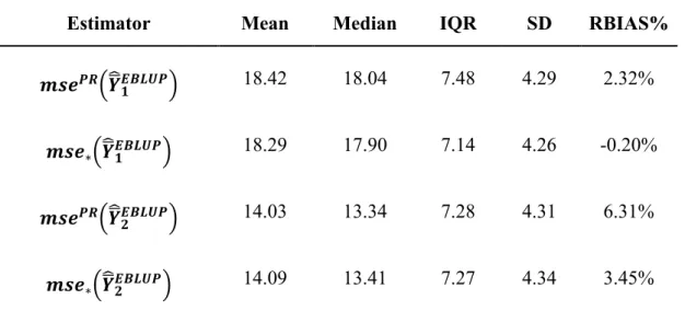
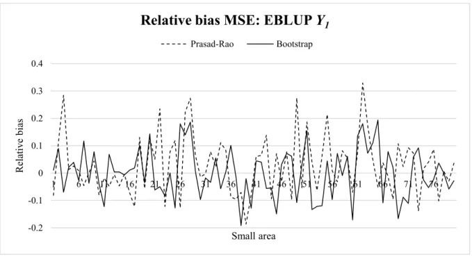
Here we compare first the MSE estimates obtained via the Prasad-Rao analytical approximation with the MSE estimates obtained by parametric bootstrap for the univariate case. Table 1 shows the descriptive statistics and bias of the Prasad-Rao and bootstrap estimators for univariate EBLUP across the small areas. It can be seen that the Prasad-Rao MSEs analytical approximations are slightly more biased than the bootstrap MSEs (by comparing the EMSE with its mean across the 𝑆 = 1,000 samples) under our scenario. Figure 1 and Figure 2 show the relative bias of the MSEs; these show that the Prasad-Rao MSE approximation slightly overestimates the true MSE for some areas. This is particularly true for 𝑌₁. For more details on the Prasad-Rao approximation compared to the bootstrap for univariate EBLUP via simulation studies we refer to González-Manteiga et al. (2008a).

--- Insert Table 1 about here

--- Insert Figure 1 about here

--- --- Insert Figure 2 about here

---In Table 2 we compare the results of the univariate with the multivariate bootstrap MSE estimation in terms of reduction in MSE and bias. We calculate the relative percentages of reduction in terms of EMSE (and bootstrap MSE) as follows: Δ_𝑑𝑘 =

16 𝐸𝑀𝑆𝐸(𝑌̅̂_𝑑𝑘𝑀𝐸𝐵𝐿𝑈𝑃)−𝐸𝑀𝑆𝐸(𝑌̅̂_𝑑𝑘𝐸𝐵𝐿𝑈𝑃)

𝐸𝑀𝑆𝐸(𝑌̅̂𝑑𝑘𝐸𝐵𝐿𝑈𝑃)

∙ 100, for 𝑑 = 1, … , 𝐷, where 𝑘 = 1,2 denotes the index of the

kth _{component of the MEBLUP means vector or the k}th _{variable in case of univariate EBLUP.}

These are shown in parentheses ( ). We also show the median across the small areas of the following quantities: empirical MSE (𝐸𝑀𝑆𝐸), bootstrap MSE estimates (𝑚𝑠𝑒_∗) and relative bias % (𝑅𝐵𝐼𝐴𝑆(𝑚𝑠𝑒_∗)%), and relative percentages of reduction in terms of EMSE (and bootstrap MSE) (𝛥𝑑). We provide the median across the small area as a robust central

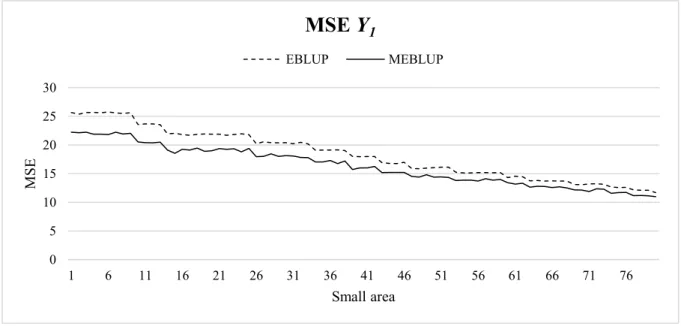
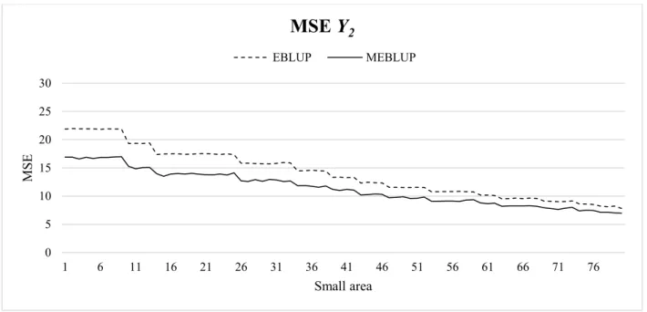
tendency index to avoid the impact of extreme values in some small areas (Giusti et al., 2013; Chambers et al., 2011). Figure 3 and Figure 4 show the comparisons of the bootstrap MSEs estimated for the EBLUPs and MEBLUPs for the opposite signs case only. It can be seen that, in line with the EMSEs, the multivariate bootstrap procedure provides predictions with lower variability than the univariate approach, and the MSE estimates show no noticeable bias across the small areas. When the population size in area d, 𝑁_𝑑, increases, 𝛥_𝑑𝑘 becomes smaller. The percentages of reduction in terms of MSE are smaller in the case of same signs of the correlation coefficients in the variance-covariance matrices.

--- Insert Table 2 about here

--- Insert Figure 3 about here

--- --- Insert Figure 4 about here

17

The percentage of reductions in terms of MSE (and EMSE) may depend on the magnitude and sign of 𝜌_𝑒 and 𝜌_𝑢 as well as the intra-class correlation coefficient. As Datta et al. (1999) points out that when 𝜌_𝑒 and 𝜌_𝑢 have opposite signs, the multivariate model performs better in terms of MSE than the univariate modelling case. It can be seen that when the signs in the variance-covariance matrices are the same the percentages of reduction in terms of MSE of the multivariate EBLUP over the univariate ones are smaller than in the case of opposite signs.

Our bootstrap procedure performs well under the model assumptions, and we can see appreciable gains in efficiency in terms of MSE over the univariate modelling. Also, we note that there is no bias in the estimates of the MSE.

5. Application to Corn and Soy Bean Data

We apply our multivariate bootstrap method to the well-known corn and soy bean data of the LANDSAT data that was used in Battese et al. (1988) comparing the multivariate and univariate models. LANDSAT comprises survey and satellite data for corn and soy beans for 12 Iowa counties, obtained from the 1978 June Enumerative Survey of the U.S. Department of Agriculture and from land observatory satellites during the 1978 growing season. The data file consists of 𝑛 = 37 observations, 𝐷 = 12 areas, and the following variables:

 CornHec: hectares of corn (𝑌₁);

 SoyBeansHec: hectares of soy beans (𝑌2);

 CornPix: number of pixels of corn in sample segment within county (𝑥₁);

18

As shown, the county means of number of pixels per segment of corn and soy beans, from satellite data, for 12 counties in Iowa are also used where we have the population size, sample size, and means of these auxiliary variables. These data files can be downloaded from Molina and Marhuenda (2015). In order to provide better modeling fit we applied Box-Cox family transformations (Box and Cox, 1964) to the response variables.

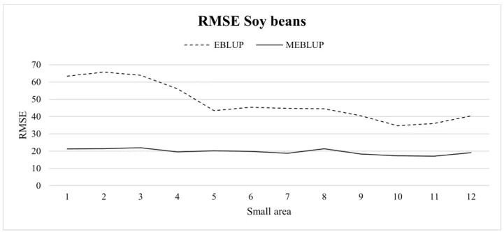
--- Insert Figure 5 about here

--- --- Insert Figure 6 about here

---Figure 5 and ---Figure 6 show the RMSE of the univariate and multivariate EBLUPs where the small areas are ordered by growing sample sizes. It can be seen that the multivariate bootstrap algorithm provides estimates with smaller variability than the univariate case as was confirmed in the simulation study. The model diagnostics show good model fitting in both cases.

6. Conclusion

In this paper we proposed the use of parametric bootstrap for estimating MSEs for vectors of means of small domains under a multivariate mixed effects model for unit-level SAE. The multivariate SAE is more appropriate than the univariate SAE in the case of correlated responses. Indeed, in this case, multivariate mixed effects models may lead to more reliable estimates than the univariate BHF model. This, of course, needs to be taken into account when estimating the MSE and hence we have proposed the parametric bootstrap for the MEBLUP. In the simulation study we assessed empirically the behaviour of our approach for

19

estimating the MSE and in particular the bias. Our results are in line with the literature and no bias is shown.

Although this paper focuses on vectors of means as the target inferential parameter, this bootstrap procedure can be extended to other quantities in a multivariate setting. Non-parametric bootstrap procedures could be studied in future work, and comparisons between the two methodologies would be useful for practitioners. Normality assumptions can be relaxed according to Hall and Maiti (2006). Furthermore, hybrid bootstrap MSE estimators should be considered. González-Manteiga et al. (2008a) studied hybrid bootstrap MSE estimators which are second-order unbiased. Other interesting extensions to this paper may involve the study of robustness to non-normality.

Acknowledgments

This research was financially supported by the UK Economic and Social Research Council (ESRC), grant number ES/J500094/1.

20

Appendix: Specification of the R functions used

Here we describe the main R packages (and functions) that we used to conduct the simulation study and application.

1. Estimation of small area means and bootstrap MSE under the univariate BHF model: ‘sae’ R package (Molina and Marhuenda, 2015):

 Required packages: nlme, MASS,

 Functions: eblupBHF( ) and pbmseBHF( ).

2. Estimation of the multivariate mixed effects model parameters (𝜮_𝑒, 𝜮_𝑢, 𝜷) described in (3): ‘mlmmm’ R package (Yucel, 2010):

21

References

Baillo, A. and Molina, I. (2009). Mean Squared Errors of Small-Area Estimators Under a Unit-Level Multivariate Model. Statistics 43:553-569.

Battese, G. E., Harter, R. M. and Fuller, W. A. (1988). An Error-Components model for Prediction of County crop areas using Survey and Satellite data. Journal of the American Statistical Association 83(401): 28-36.

Box, G. E. P. and Cox, D. R. (1964). An analysis of transformations. Journal of Royal Statistical Society Series B 26:211-246.

Chambers, R., Chandra, H., and Tzavidis (2011). On bias-robust mean squared error estimation for pseudo-linear small area estimators. Survey Methodology 37:153-170. Das, K., Jiang, J. and Rao, J.N.K. (2004). Mean Squared Error of Empirical Predictor. Annals

of Statistics 32:818-840.

Datta, G. S., Day, B. and Basawa, I. (1999). Empirical best linear unbiased and empirical Bayes prediction in multivariate small area estimation. Journal of Statistical Planning and Inference 75:269-279.

Datta, G.S. and Lahiri, P. (2000). A Unified Measure of Uncertainty pf Estimated Best Linear Unbiased Predictors in Small Area Estimation Problems. Statistica Sinica 10:613-627. Efron, B. and Tibshirani, R. (1993). An Introduction to the Bootstrap. London: Chapman and

Hall.

Fuller, W. A. and Harter, R. M. (1987). The Multivariate Components of Variance Model for Small Area Estimation, in R. Platek, J. N. K. Rao, C. E. Sarndal, and M. P. Singh (Eds.),

Small Area Statistics, New York: Wiley, 103-123.

González-Manteiga, W., Lombardía, M. J., Molina, I., Morales, D. and Santamaría, L. (2008a). Bootstrap Mean Squared Error of a Small-Area EBLUP. Journal of Statistical Computation and Simulation 78:443-462.

González-Manteiga, W., Lombardía, M. J., Molina, I., Morales, D. and Santamaría, L. (2008b). Analytic and bootstrap approximations of prediction errors under multivariate Fay-Herriot model. Computational Statistics and Data Analysis 52:5242-5252.

Giusti, C., Tzavidis, N., Pratesi, M. And Salvati, N. (2013) Resistance to Outliers pf M-Quantile and Robust Random Effects Small Area Models. Communications in Statistics

22

– Simulation and Computation 43:549-568.

Hall, P. (1992). The Bootstrap and Edgeworth Expansion. New York: Springer.

Hall, P. and Maiti, T. (2006). Nonparametric Estimation of Mean-Sqaured Prediction Error in Nested-Error Regression Models. Annals of Statistics 34:1733-1750.

Kackar, R.N. and Harville, D.A. (1981). Unbiasedness of Two-Stage Estimation and prediction Procedure for Mixed Linear Models. Journal of the American Statistical Association 79:853-862.

Marchetti, S., Tzavidis, N. and Pratesi, M. (2012). Non-parametric Bootstrap Mean Squared Error Estimation for M-quantile Estimators of Small Area Averages, Quantiles and Poverty Indicators. Computational Statistics and Data analysis 56:2889-2902.

Mardia, K. V., and Marshall, R. J. (1984). Maximum Likelihood Estimation of Models for Residual Covariance in Spatial Regression. Biometrika 71(1).

Molina, I. (2009). Uncertainty under a multivariate nested-error regression model with logarithmic transformation. Journal of Multivariate Analysis 100:963-980.

Molina, I., and Marhuenda, Y. (2015). sae: An R Package for Small Area Estimation. The R Journal 7(1):81-98.

Prasad, N.G.N. and Rao, J.N.K. (1990). The Estimation of Mean Squared Error of Small-Area Estimators. Journal of the American Statistical Association 85:163-171.

Rao, J. N. K. and Molina, I. (2015). Small area estimation. New York: Wiley.

Schafer, J. L., and Yucel, R. M. (2002). Computational Strategies for Multivariate Linear Mixed-Effects Models With Missing Values. Journal of Computational and Graphical Statistics 11:437-457.

Sweeting, T. J. (1980). Uniform Asymptotic Normality of the Maximum Likelihood Estimator. The Annals of Statistics 8.

Yucel, R. (2010) mlmmm: ML estimation under multivariate linear mixed models with missing values. R package version 0.3-1.2. Retrieved from http://CRAN.R-project.org/package=mlmmm.

23

Tables and Figures

Estimator Mean Median IQR SD RBIAS%

𝒎𝒔𝒆𝑷𝑹(𝒀̅̂_𝟏𝑬𝑩𝑳𝑼𝑷) 18.42 18.04 7.48 4.29 2.32%

𝒎𝒔𝒆_∗(𝒀̅̂_𝟏𝑬𝑩𝑳𝑼𝑷) 18.29 17.90 7.14 4.26 -0.20%

𝒎𝒔𝒆𝑷𝑹(𝒀̅̂_𝟐𝑬𝑩𝑳𝑼𝑷) 14.03 13.34 7.28 4.31 6.31%

𝒎𝒔𝒆∗(𝒀̅̂𝟐𝑬𝑩𝑳𝑼𝑷) 14.09 13.41 7.27 4.34 3.45%

Table 1 Descriptive statistics and relative bias of the Prasad-Rao and bootstrap estimators for univariate EBLUP MSE across small areas, 𝑬𝑴𝑺𝑬(𝒀̅̂_𝟏𝑬𝑩𝑳𝑼𝑷) = 𝟏𝟕. 𝟗𝟖,

𝑬𝑴𝑺𝑬(𝒀̅̂_𝟐𝑬𝑩𝑳𝑼𝑷) = 𝟏𝟐. 𝟕𝟓, for 𝝆_𝒆 = −𝟎. 𝟕 and 𝝆_𝒖 = 𝟎. 𝟑. Correlation structure Performance measure EBLUP MEBLUP 𝒀𝟏 𝒀𝟐 𝒀𝟏 𝒀𝟐 𝝆_𝒆= −𝟎. 𝟕, 𝝆𝒖= 𝟎. 𝟑 EMSE 17.98 12.75 16.26 (-9.25) 10.62 (-17.63) 𝒎𝒔𝒆_∗ 17.90 13.41 16.34 (-9.40) 11.12 (-17.48) 𝑹𝑩𝑰𝑨𝑺(𝒎𝒔𝒆∗)% -0.20% 3.45% -0.06% 1.50% 𝝆_𝒆 = 𝟎. 𝟕, 𝝆_𝒖= 𝟎. 𝟑 EMSE 17.27 12.64 17.43 (1.10%) 12.06 (-6.25%) 𝒎𝒔𝒆_∗ 18.07 13.38 17.88 (-1.41) 12.21 (-.9.00%) 𝑹𝑩𝑰𝑨𝑺(𝒎𝒔𝒆_∗)% 3.56% 6.41% 1.72% 2.55%

24

Table 2 Empirical mean squared error, bootstrap MSE, relative bias median results across the small areas: EBLUP and MEBLUP estimates – parametric bootstrap. (𝜟_𝒌

shown in parenthesis).

Figure 1 Relative bias of univariate EBLUPs’ MSEs of 𝒀_𝟏 estimated via Prasad-Rao approximation and parametric bootstrap for 𝝆_𝒆 = −𝟎. 𝟕 and 𝝆_𝒖 = 𝟎. 𝟑, ordered by increasing 𝑵_𝒅. -0.2 -0.1 0 0.1 0.2 0.3 0.4 1 6 11 16 21 26 31 36 41 46 51 56 61 66 71 76 R elativ e bias Small area

Relative bias MSE: EBLUP Y

25

Figure 2 Relative bias of univariate EBLUPs’ MSEs of 𝒀𝟐 estimated via Prasad-Rao

approximation and parametric bootstrap for 𝝆_𝒆 = −𝟎. 𝟕 and 𝝆_𝒖 = 𝟎. 𝟑, ordered by increasing 𝑵_𝒅.

Figure 3 Bootstrap MSEs 𝒀_𝟏: comparison between EBLUP and MEBLUP 𝝆_𝒆 = −𝟎. 𝟕

and 𝝆𝒖 = 𝟎. 𝟑, ordered by increasing 𝑵𝒅. -0.2 -0.1 0 0.1 0.2 0.3 0.4 1 6 11 16 21 26 31 36 41 46 51 56 61 66 71 76 R elativ e bias Small area

Relative bias MSE: EBLUP Y

Prasad-Rao Bootstrap 0 5 10 15 20 25 30 1 6 11 16 21 26 31 36 41 46 51 56 61 66 71 76 MSE Small area

MSE Y

26

Figure 4 Bootstrap MSEs 𝒀_𝟐: comparison between EBLUP and MEBLUP 𝝆_𝒆 = −𝟎. 𝟕

and 𝝆𝒖 = 𝟎. 𝟑 ordered by increasing 𝑵𝒅.

Figure 5 Bootstrap RMSEs corn: comparison between EBLUP (---) and MEBLUP (__).

0 5 10 15 20 25 30 1 6 11 16 21 26 31 36 41 46 51 56 61 66 71 76 MSE Small area

MSE Y

RMSE Corn

27

Figure 6 Bootstrap RMSEs soy beans: comparison between EBLUP (---) and MEBLUP (__). 0 10 20 30 40 50 60 70 1 2 3 4 5 6 7 8 9 10 11 12 R MSE Small area

RMSE Soy beans