A. Binary-Constraint
Search Algorithm
for Minimizing
Hardware
during
Hardware/Software
Partitioning
Frank Vahidf Jie Gong and Daniel D. Gajski Department of Information and Computer Science
University of California, Irvine, CA, 92717
Abstract
Partitioning a system ‘3 functionality among interact- ing hardware and software components is an important part of system design. We introduce a new partitioning approach that caters to the main objective of the hard- ware/software partitioningproblem, i.e., minimizing hard- ware ,for given performance constraints. We demonstrate results superior to those of previously published algorithms
intendedjor hardware/software partitioning. The approach
may be genera&able to problems in which one metric must be minimized while other metrics must merely satisfy con-
straints.
1
Introduction
Co.mbined hardware/software implementations are common in embedded systems. Software running on an existing processor is less expensive, more easily modi- fiable, and more quickly designable than an equivalent application-specific hardware implementation. However,
hardware may provide better performance. A system de- signer’s goal is to implement a system using a minimal amount of application-specific hardware, if any at all, to satisfy required performance. In other words, the designer attempts lo implement as much functionality as possible in software.
Deficiencies of the much practiced ad-hoc approach to partitioning have led to research into more formal, algo- rithmic approaches. In the ad-hoc approach, a designer starts with an informal functional description of the de- sired system, such as an English description. Based on
previous experience and mental estimations, the designer partitions the functionality among hardware and software components, and the components are then designed and integrated. This approach has two key limitations. First, due to limited time, the designer can only consider a small numbe.r of possible partitionings, so many good solutions
will never be considered. Second, the effects that partition-
ing has on performance are far too complex for a designer to accurately estimate mentally. As a result of these limi- tations, designers often use more hardware than necessary to ensure performance constraints are met.
--
tF. V&id . IS presently with the Department of Computer
Science, University of California, Riverside, CA 92521.
In formal approaches, one starts with a functional de- scription of the system in a machine-readable language, such as VHDL. After verifying, usually through simula- tion, that the description is correct, the functionality is decomposed into functional portions of some granularity. These portions, along with additional information such as data shared between portions, make up an internal model of the system. Each portion is mapped to either hardware or software by partitioning algorithms that search large numbers of solutions. Such algorithms are guided by au- tomated estimators that evaluate cost junctions for each partitioning. The output is a set of functional portions to be mapped to software and another set to be mapped to hardware. Simulation of the designed hardware and com- piled software can then be performed to observe the effects of partitioning. Figure 1 shows a typical configuration of a hardware/software partitioning system.
FU-CWld duaiplm
Figure 1: Basics parts of a hw/sw partitioning system
The partitioning algorithm is a crucial part of the for- mal approach because it is the algorithm that actually min- imizes the expensive hardware. However, current research into algorithms for hardware/software partitioning is at an early stage. In [l], the essential criteria to consider dur- ing partitioning are described, but no particular algorithm is given. In [2], certain partitioning issues are also de- scribed but no algorithm is given. In [3], an approach based on a multi-stage clustering algorithm is described, where the closeness metrics include hardware sharing and con- currency, and where particular clusterings are evaluated based on factors including an area/performance cost func- tion. In [4], an algorithm is described which starts with most functionality in hardware, and which then moves por-
sign. In [5], an approach is described which starts with all functionality in software, and which then moves portions into hardware using an iterative-improvement algorithm such as simulated annealing. The authors hypothesize that starting with an all-software partitioning will result in less final hardware than starting with all-hardware partition- ing (our results support this hypothesis). In [6], simulated annealing is also used. The focus is on placing highly uti- lized functional portions in hardware. However, there is no direct performance measurement. The common short- coming of all previous approaches is the lack of advanced methods to minimize hardware.
We propose a new partitioning approach that specifi- cally addresses the need to minimize hardware while meet- ing performance constraints. The novelty of the approach is in how it frees a partitioning algorithm, such as simu- lated annealing, from simultaneously trying to satisfy per- formance constraints and to minimize hardware, since try- ing to solve both problems simultaneously yields a poor solution to both problems. Instead, in our approach, we use a relaxed cost function that enables the algorithm to focus on satisfying performance, and we use an efficiently- controlled outer loop (based on binary-search) to han- dle the hardware minimization. As such, our approach can be considered as a meta-algorithm that combines the binary-search algorithm with any given partitioning algo- rithm. The approach results in substantially less hard- ware, while using only a small constant factor of additional computation and still satisfying performance constraints (whereas starting with an all-software partition and apply- ing iterative-improvement algorithms often fails to satisfy performance). Such a reduction can significantly decrease implementation costs. Moving one of the subproblems to an outer loop may in fact be a general solution to other problems in which one metric must be minimized while others must merely satisfy constraints.
The paper is organized as follows. Section 2 gives a definition of the hardware/software partitioning problem. Section 3 describes previous hardware/software partition- ing algorithms, an extension we have made to one previ- ous algorithm to reduce hardware, and our new hardware- minimizing algorithm based on constraint-search. Sec- tion 4 summarizes our experimental results on several ex- amples.
2
Problem
Definition
While the partitioning subproblem interacts with other subproblems in hardware/software codesign, it is distinct, i.e., it is orthogonal to the choice of specification language, the level of granularity of functional decomposition, and the specific estimation models employed.
We are given a set of functional objects 0 =
{01,02,..., on} which compose the functionality of the sys-
tem under design. The functions may be at any of various levels of granularity, such as tasks (e.g., processes, pro- cedures or code groupings) or arithmetic operations. We are also given a set of performance constraints Cons =
{Cl,C2 ,..., Cm), where Cj = {G, timecon}, G C 0, and
limecon E Posihve. hvnecon is a constraint on the maxi- mum execution-time of the all functions in group G. It is simple to extend the problem to alIow other performance constraints such as those on bitrates or inter-operation de- lays, but we have not included such constraints in order to simplify the notation.
A hardware/software partition is defined as two sets H and S, where H C 0, S C 0, H US = 0, HnS=O.Th is e ni ion does not prevent further par- dfi t tition of hardware or software. Hardware can be parti- tioned into several chips while software can be executed on more than one processor. The hardware size of H, or Hsite(H) is defined as the size (e.g., transistors) of the hardware needed to implement the functions in H. The performance of G, or Performance(G), is defined as the total execution time for the group of functions in G for a given partition H,S. A performance satisfying parti- tion is one for which Performance(Cj.G) 5 Cj.timecon for all j = 1 . . . m.
Deflnition 1: Given 0 and Cons, the Hard- ware/Software Partitioning Problem is to find a per- formance satisfying partition H and S such that Hsize(H) is minimal. In other words, the problem is to map all the functions to either hardware or software in such a way that we find the minimal hardware for which all perfor- mance constraints can still be met. Note that the hard- ware/software partitioning problem, like other partitioning problems, is NP-complete.
The all-hardware size of 0 is defined as the size of an all-hardware partition, or in other words as Hsize(0). Note that if an all-hardware partition does not satisfy per- formance constraints, no solution exists.
To compare any two partitions, a cost function is re- quired. A cost function is a function Cod(H, S, Cons, I) which returns a natural number that summarizes the overall goodness of a given partition, the smaller the better. I contains any additional information that is not contained in II, S or Cons. We define an it- erative improvement partitioning algorithm as a procedure PadAlg( H, S, Cons, I, Cost()) which returns a partition H’, S’ such that Cosl(H’, S’, Cons,I) 5 Cost( H, S, Cons, I). Examples of such algorithms include group migration [7] and simulated annealing [8].
Since it is not feasible to implement the hardware and software components in order to determine a cost for each possible partition generated by an algorithm, we assume that fast estimators are available [9, 10, 111.
3
Part it ioning solution
3.1 Basic algorithmsOne simple and fast algorithm starts with an initial partition, and moves objects as long as improvement OC-
curs. The algorithm presented in [4], due to Gupta and DeMicheli, and abbreviated as GD, can be viewed as an extension of this algorithm which ensures performance con- straints are met. The algorithm starts by creating an all- hardware partition, thus guaranteeing that a performance
satisfying partition is found if it exists (actually, certain functions which are considered unconstrainable are ini- tially placed in software). To move a function requires not only cost improvement but also that all performance con- straints still be satisfied (actually they require that max- imum interfacing constraints between hardware and soft- ware be satisfied). Once a function is moved, the algorithm tries to move closely related functions before trying others.
Greedy algorithms, such as the one described above, suffer from the limitation that they are easily trapped in a local minimum. As a simple example, consider an ini- tial partition that is performance satisfying, in which two heavily communicating functions or and 02 are initially in hardware. Suppose that moving either 01 or 02 to soft- ware results in performance violations, but moving both 01 and 02 results in a performance satisfying partition. Neither of the above algorithms can find the latter solu- tion because doing so requires accepting an intermediate, seemmgly negative move of a single function.
To overcome the limitation of greedy algorithms, oth- ers have proposed using an existing hill-climbing algorithm such as simulated annealing. Such an algorithm accepts some number of negative moves in a manner that over- comes many local minimums. One simply creates an initial partit,ion and applies the algorithm.
In [5], such an approach is described by Ernst and Henkel that uses an all-software solution for the initial par- tition. A hill-climbing partitioning algorithm is then used to extract functions from software to hardware in order to meet performance. The authors reason that such ex- traction should result in less hardware than the approach where functions are extracted in the other direction, i.e., from bardware to software.
Cost function
We now consider devising a cost function to be used by the hill-climbing partitioning algorithm. The difficultly lies in trying to balance the performance satisfiability and hardware minimization goals. The GD approach does not encounter this problem since performance satisfiabiiity is not part of the cost function. The cost function is only used to evaluate partitions that already satisfy the perfor- mance constraints. The algorithm simply rejects all par- titions that are not performance satisfying. We saw that this approach will become trapped in a local minimum. The Ernst/Henkel approach does not encounter this prob- lem since hardware size is not part of the cost function; instead, it is fixed beforehand, by allocating resources be- fore partitioning. This approach requires the designer to manually try numerous hardware sizes, reapplying parti- tioning for each, to try to find the smallest hardware size that yields a performance satisfying partition.
We propose a third solution. We use a cost function with two terms, one indicating the sum of all performance violations, the other the hardware size. The performance term is weighed very heavily to ensure that a performance satisfying solution is found, so minimizing hardware is a secondary consideration. The cost function is:
Cost( H, S, Cons) = kperf Violation(C.,)
J”1 + k OPeD x Hsize(H)
where Violation(Cj) = Performance(CJ.G)-Cj.timecon if the difference is greater than 0, else Violadion(C,) = 0. Also, kperf >> k,,,,, but kperf should not be infinity, since then the algorithm could not distinguish a partition which almost meets constraints from one which greatly violates constraints.
We refer to this solution as the PWHC (performance- weighted hi-climbing) algorithm. We shall see that it gives excellent results as compared to the GD algorithm, but there is still room for improvement. In particular, when starting with an all-software partition, hill-climbing algorithms often fail to find a performance-satisfying solu- tion.
3.2
A new constraint-search
approach
While incorporating performance and hardware size considerations in the same cost function, as in PWHC, tends to gives much better results than previous ap proaches, we have determined a superior approach for min- imizing hardware. Our approach involves dec0uplin.g to a degree the problem of satisfying performance from the problem of minimizing hardware.3.2.1 Foundation
The first step is to realize that the difficulty experienced in PWHC is that the two metrics in the cost function, performance and hardware size, directly compete with each other. In other words, decreasing performance violations usually increases hardware size, while decreasing hardware size usually increases performance violations. An iterative- improvement algorithm has a hard time making significant progress towards minimizing one of the metrics since any reduction in one metric’s value yields an increase in the other metric’s value, resulting in very large “hills” that must be climbed. To solve this problem, we can relax the cost function goal. Rather than minimizing size, we just wish to find any size below a given constraint C,,,,.
Cost ( H, S, Cons, Csize ) m
= k P-f x c Violation(C,)
j=1
+ k area x Violation(Hsize( H), Csize)
It is no longer required that kperf >> kare,,. We set k Per! - - k,,,, = 1. The effect of relaxing the cost function
goal is that once the hardware size drops below the con- straint, decreasing performance violations does not neces- sarily yield a hardware-size violation; hence the iterative- improvement algorithm has more flexibility to work to- wards eliminating performance violations.
The hardware minimization problem can now be stated distinct from the partitioning problem.
Deflnition 2: Given 0, Cons, PartAlg() and Cosl(), the Minimal Hardware-Constraint Prob- lem is to determine the smallest Csire such that Cost(PartAlg(H, S, COTIS, Csize, Cost()),Cons, Csize) = 0. In other words, we must choose the smallest size con- straint for which a performance satisfying solution can be found by the partitioning algorithm.
Theorem 1: Let PartAlg() be such that it al- ways finds a zero-cost solution if one exists. Then Cost(PartAlg(H, S, Cons, Csize, Cost()), Cons, Csize) = 0 implies that Cost( PartAlg( H, S, Cons, Csize + 1, Cost()), COTZS, Csize + 1) = 0.
Proof: we can create a (hypothetical) algorithm which subtracts 1 from its hardware-size constraint if a zero-cost solution is not found. Given Csize + 1 as the constraint, then if a zero-cost is not found, the algorithm will try Csize as the constraint. Thus the algorithm can always find a zero-cost solution for Csile + 1 if one exists for Csile.
The above theorem states that if a zerocost solution is found for a given Csize, then zerocost solutions will be found for all larger values of Csire also. From this theorem we see that the sequence of cost numbers ob- tained for C *,ze = 0, 1, . ..) AllHardwareSiae consists of z non-zero numbers followed by Ceil= - z zero’s, where z E {O..A~~HardwareSize}. Let CostSequence equal this sequence of cost numbers. Figure 2 depicts an example of a CostSequence graphically. (It is important to note that CostSequence is conceptual; it describes the solu- tion space, but we do not actually need to generate this sequence to find a solution). We can now restate the min- imal hardware-constraint problem as a search problem:
mr zwo
CUSf 500 200 300 350 50 b 0 . . 0 0
Size H++i+++FH
conatraht 0 1 2 3 4 5 6 AllHardwareSlze
Figure 2: An example cost sequence
Deflnition 3: Given H, S, Cons, PattAlg() and Cost0 the Minimal Hardware-Constraint Search Problem is to find the first zero in CostSequence.
Given this definition, we see that the problem can be easily mapped to the well-known problem of Sorted-array search, i.e., of finding the first occurrence of a key in an ordered array of items. The main difference between the two problems is that whereas in sorted-array search the items exist in the array beforehand, in our constraint- search problem an item is added (i.e. partitioning applied and a cost determined) only if the array location is visited during search. In either case, we wish to visit as few ar- ray items as possible, so the difference does not affect the solution. A second difference is that the first z items in CostSequence are not necessarily in increasing or decreas- ing order. Since we are looking for a zero cost solution,
we don’t care what those non-zero values are, so we can convert CostSequence to an ordered sequence by mapping each non-zero cost to 1.
The constraint corresponding to the first zero cost rep- resents the minimal hardware, or optimal solution to the partitioning problem. Due to the NP-completeness of par- titioning, it should come as no surprise that we can not actually guarantee an optimal solution. Note that we as- sumed in the above theorem that PatlAlg() finds a zero- cost solution if one exists for the given size constraint. Since partitioning is NP-complete, such an algorithm is impractical. Thus PartAlg() may not find a zero-cost so- lution although one may exist for a given size constraint. The result is that the first zero in CostSequence may be for a constraint which is larger than the optimal, or that non-zero costs may appear for constraints larger than that yielding the first zero cost, meaning the sequence of zeros contains spikes. However, the first zero cost should corre- spond to a constraint near the optimal if a good algorithm is used. In addition, any spikes that occur should also only appear near the optimal. Thus the algorithm should yield near optimal results.
It is well-known that binary-search is a good solution to the sorted-array search problem, since its worst case behavior is log(N) for an array of N items. We.therefore incorporate binary-search into our algorithm.
3.2.2 Algorithm
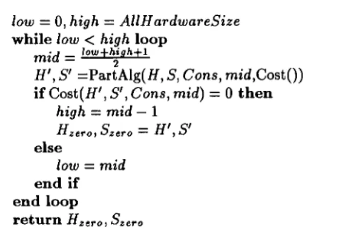
We now describe our hardware-minimizing partitioning al- gorithm based on binary-search of the sequence of costs for the range of possible hardware constraints, which we refer to as the BCS (binary constraint-search) algorithm. The algorithm uses variables low and high which indicate the current window of possible constraints in which a zero-cost constraint lies, and variable mid which represents the mid- dle of that window. Variables H,,,, and S,,,, store the zero-cost partition which has the smallest hardware con- straint so far encountered.
Algorithm 3.1 BCS hw/sw partitioning
low = 0, high = AllHardwareSize
while low < high loop
,,,id = low+high+l
H’, S’ =PariAlg(H, S, Cons, mid,Cost())
if Cost(H’, S’, Cons, mid) = 0 then
high = mid - 1 H zet.0, S,,,, = H’,S’ else low = mid end if end loop return Hz,,, , Lo
The algorithm performs a binary search through the range of possible constraints, applying partitioning and
then the cost function as each constraint is “visited”. The algorithm looks very much like a standard binary-search algorithm with two modifications. First, mid is used as a hardware constraint for partitioning whose result is then used to determine a cost, in contrast to using mid as an index to an array item. Second, the cost is compared to 0, in contrast to an array item being compared to a key.
3.2.;3 Reducing runtime in practice
After experimentation, we developed a simple modification of t.he constraint-search algorithm to reduce its runtime in pract.ice. Let SiZebest be the smallest zerocost hardware const.raint. If a Csize constraint much larger than SiZebest
is provided to PartAIg(), the algorithm usually finds a so- lution very quickly. The functions causing a performance violation are simply moved to hardware. If a Csile con- straint much smaller than SiZebest is provided, the algo- rithm also stops fairly quickly, since it is unable to find a sequence of moves that improves the cost. However, if Csize is slightly smaller or larger than SiZebest, the algo- rithm usually makes a large number of moves, gradually inching its way towards a cost of zero. This situation is very qdifferent from traditional binary-search where a com- parison of the key with an item takes the same time for any item. Near the end of binary-search the window of possible constraint values is very small, with SiZebesr some- where inside this window. Much of the constraint-search algorithm’s runtime is spent reducing the window size by minute amounts and reapplying lengthy partitioning.
In practice, we need not find the smallest hardware size to such a degree of precision. We thus terminate the binary-search when the window size (i.e., high - low) is less than a certain percentage of AIIHardurareSize. This percentage is called a precision factor. We have found that a precision factor of 1% achieves a speedup of roughly 2.5; we allow the user to select any factor.
X2.4: Complexity
The worst-case runtime complexity of the constraint- search algorithm equals the complexity of the chosen parti- tioning algorithm PartAlg() multiplied by the complexity of our binary constraint-search. While the complexity of the binary search of a sequence with AllHardwareSize
items is logz(AllHardwareSize), the precision factor re- duces this to a constant.
Theorem 2: The complexity of the binary search of an N element CostSequence with a precision factor a is loch($).
Proof: We start with a window size of N, and repeat- edly divide the window size by 2 until the window size equals. a x N. Let w be the number of windows generated;
w will thus give us the complexity. An equivalent value for w is obtained by starting with a window size of a x N, and multiplying the size by 2 until the size is N. Hence we obtain the following equation: (a x N) x 2’” = N. Solving
for w yields w = logs( 5) = logz( a). The complexity is therefore logz(i).
We see that binary constraint-search partitioning with a precision factor has the same theoretical complexity as the partitioning algorithm PartAlg(). In practice, the binary constraint-search contributes a small constant factor. For example, a precision factor of 5% results in a constant
factor of logs(20) = 4.3.
4
Experiments
We briefly describe the environment used to compare the various algorithms on real examples. It is important to note that most environment issues are orthogonal t.o the issue of algorithm design. Our algorithms should perform
well in any of the environments discussed in other work such as [II 2, 3,4,5]. It should also be noted that any par- titioning algorithm can be used within the BCS algorithm, not just simulated annealing.
We take a VHDL behavioral description as input. The description is decomposed to the granularity of tasks, i.e., processes, procedures, and optionally to statement blocks such as loops. Large data items (variables) are also treated as functions. Estimators of hardware size and behavior execution-time for both hardware and software are avail- able [9, lo]. These estimators are especially designed to be used in conjunction with partitioning. In particular, very fast and accurate estimations are made available through special techniques to incrementally modify an estimate when a function is moved, rather than reestimating en- tirely for the new partition. The briefness of our discuission on estimation does not imply that it is trivial or simple, but instead that it is a different issue not discussed in this paper. We also note here that ILP solutions are inadeq,uate for use here because the metrics involved are non-linear, since they are obtained by using sophisticated estimators based on design models, rather than by using linear but grossly inaccurate metrics.
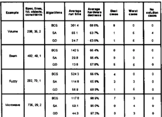
We implemented three partitioning algorithms: GD, PWHC, and BCS. The PartAIg() used in PWHC and BCS is simulated annealing. From now on, we also refer the PWHC algorithm as SA (Simulated Annealing). The pre- cision factor used in BCS is 5%. We applied each algori.thm to several examples: a real-time medical system (Volume) for measuring volume, a beam former system (Beam), a fuzzy logic control system (Fuzzy), and a microwave trans- mitter system (Microwave). For each example, a varie,ty of performance constraints were input. Some examples have performance constraints on one group of tasks in the sys- tem. Others have performance constraints on two groups of tasks in the system. We tested each example using ;s set of performance constraints that reside between the time re- quired for an all-hardware partition and the time requ.ired for an all-software partition. The initial partition used in each trial by SA and BCS is an all-software partition. We also ran SA and BCS starting with an all-hardware par- tition, but found that the results were inferior to those starting with an all-software partition.
Figure 3 summarizes the results. The Average run lime is the measured CPU time running on a Sparc2. The Au-
~*__171._11
T if 1;; 1 ; 1 ; 1 ;
Figure 3: Partitioning results on industry examples
which each algorithm reduces the hardware, relative to the
size of an all-hardware implementation. The Best cases is
the number of times the given algorithm results in a hard-
ware size smaller than those of both other algorithms. The
Worst cases is the number of times the algorithm results
in a hardware size that is larger than those of both other
algorithms. No solution cases is the number of times the
algorithm fails to find a performance-satisfying partition.
The results demonstrate the superiority of the BCS al-
gorithm in finding a performance-satisfying partition with
minimal hardware. BCS always finds a performance-
satisfying partition (in fact, it is guaranteed to do so),
whereas SA failed in 5 cases, which is 13.2% of all cases.
While GD also always finds a performance-satisfying par-
tition, BCS results in a 9.5% savings in hardware, cor-
responding to an average savings of approximately 12083
gates [12]. An additional positive note that can be seen
from the experiments is that the increase in computation
time of BCS over simulated annealing is only 4.1, slightly
better than the theoretical expectation of 4.3.
To further evaluate the BCS algorithm, we developed a
general formulation of the hardware/software partitioning
problem. This formulation enables us to generate problems
that imitate real examples, without spending the many
months required to develop a real example. In addition,
the formulation enables a comparison of algorithms with-
out requiring use of sophisticated software and hardware
estimators, which makes algorithm comparison possible for
others who do not have such estimators. We generated 125
general hardware-software partitioning problems, and then
applied BCS with a 5% precision factor, SA and GD. The
BCS algorithm again finds performance-satisfying parti-
tions with less hardware. SA failed to find a performance-
satisfying partition in 15 cases, which is 12.5% of all cases.
While GD also always found a performance-satisfying par-
tition, BCS resulted in nearly a 10% savings in hardware.
Figure 4 summarizes the comparison of BCS to the other
algorithms. Details of the formulation, the psuedorandom
hardware/software problem generation algorithm, and the
partitioning results are provided in [13].
Hardware Hardware Failure rate Time increase
(SA) “~% 8flvdR dKG-
4.1x 2.7% 9.5% 12.5%
Figure 4: BCS compared to other algorithms
5
Conclusion
The BCS algorithm excels over previous hard-
ware/software partitioning algorithms in its ability to min-
imize hardware while satisfying performance constraints.
The computation time required by the algorithm is well
within reason, especially when one considers the great ben-
efits obtained from the reduction in hardware achieved by
the algorithm, including reduced system cost, faster de-
sign time, and more easily modifiable final designs. The
BCS approach is essentially a meta-algorithm that removes
from a cost function one metric that must be minimized,
and thus the approach may be applicable to a wide range
of problems involving non-linear, competing metrics.
References
[l] D. Thomas, J. Adams, and H. Schmit, “A model
and methodology for hardware/software codesign,” in
IEEE Design d Test of Computers, pp. 6-15, 1993.
[2] A. Kalavade and E. Lee, “A hardware/software code-
sign methodology for DSP applications,” in IEEE De-
sign f4 Test of Computers, 1993.
[3] X. Xiong, E. Barros, and W. Rosentiel, “A method
for partitioning unity language in hardware and soft-
ware,” in EuroDAC, 1994.
[4] R. Gupta and G. DeMicheli, uSystem-level synthe-
sis using re-programmable components,” in EDAC,
pp. 2-7, 1992.
[5] R. Ernst and J. Henkel, “Hardware-software code-
sign of embedded controllers based on hardware ex-
traction,” in International Workshop on Hardware-
Software Co-Design, 1992.
[6] Z. Peng and K. Kuchcinski, “An algorithm for par-
titioning of application specific systems,” in EDAC,
pp. 316-321, 1993.
[7] B. Preas and M. Lorenzetti, Physical Design flu-
tomation of VLSI Systems. California: Ben-
jamin/Cummings, 1988.
[8] S. Kirkpatrick, C. Gelatt, and M. P. Vecchi, “Opti-
mization by simulated annealing,” Science, vol. 220,
no. 4598, pp. 671-680, 1983.
[9] J. Gong, D. Gajski, and S. Narayan, “Software esti-
mation from executable specifications,” in Journal of
Computer and Software Engineering, 1994.
[lo] S. Narayan and D. Ga’ski, “Area and performance es-
timation from system- eve1 specifications.” i UC Irvine,
Dept. of ICS, Technical Report 92-16,1992.
[ll] W. Ye, R. Ernst, T. Benner, and J. Henkel, “Fast
timing analysis for hardware-software co-synthesis,”
in ICCD, pp. 452-457, 1993.
[12] Lf[lOO 1.5 Micron CMOS Datapath Cell Library,
[13] F. Vahid, J. Gong, and D. Gajski, “A hardware-
software partitioning algorithm for minimizing hard-
ware.” UC Irvine, Dept. of ICS, Technical Report 93-