Replicating DeepMind StarCraft II reinforcement learning benchmark with actor-critic methods

UNIVERSITY OF TARTU

Faculty of Science and Technology

Institute of Mathematics and Statistics

Mathematical Statistics

Roman Ring

Replicating DeepMind StarCraft II

Reinforcement Learning Benchmark

with Actor-Critic Methods

Bachelor’s Thesis (9 EAP)

Supervisors: Ilya Kuzovkin, MSc

Tambet Matiisen, MSc

Replicating DeepMind StarCraft II Reinforcement Learning Benchmark with Actor-Critic Methods

Bachelor’s thesis Roman Ring

Abstract. Reinforcement Learning (RL) is a subfield of Artificial Intelligence (AI) that deals with agents navigating in an environment with the goal of maximizing total reward. Games are good environments to test RL algorithms as they have simple rules and clear reward signals. Theoretical part of this thesis explores some of the popular classical and modern RL approaches, which include the use of Artificial Neural Network (ANN) as a function approximator inside AI agent. In practical part of the thesis we implement Advantage Actor-Critic RL algorithm and replicate ANN based agent described in [Vinyals et al., 2017]. We reproduce the state-of-the-art results in a modern video game StarCraft II, a game that is considered the next milestone in AI after the fall of chess and Go.

Keywords: reinforcement learning, artificial neural networks CERCS research specialisation: P176 Artificial intelligence

DeepMind’i StarCraft II stiimulõppe tulemuste reprodutseerimine aktor-kriitik meetoditega

Bakalaureusetöö Roman Ring

Lühikokkuvõte. Stiimulõpe on tehisintellekti valdkond, mille uurimisobjektiks on agent, mis navigeerib etteantud keskkonnas eesmärgiga maksimeerida oma tegevustest tulenevat preemiat. Mängud on sobivad keskkonnad stiimulõppe algo-ritmide testimiseks, kuna nendel on lihtsad reeglid ja selgelt defineeritud preemia. Töö teoreetilises osas uuritakse stiimulõppe populaarsemaid meetodeid, s.h. tehis-närvivõrkude kasutust. Praktilises osas on realiseeritud tehisnärvivõrgul põhinev aktor-kriitik algoritm [Vinyals et al., 2017]. Töös reprodutseeritakse hetke pari-maid tulemusi videomängus StarCraft II, mida peetakse tehisintellekti valdkonna järgmiseks verstapostiks pärast male ja Go alistamist.

Märksõnad: stiimulõpe, tehisnärvivõrgud CERCS teaduseriala: P176 Tehisintellekt

Contents

Introduction 4

1 Background 6

1.1 Reinforcement Learning . . . 6

1.1.1 Markov Decision Process . . . 8

1.1.2 Credit Assignment Problem . . . 9

1.1.3 Value-Based Methods . . . 10

1.1.4 Policy-Based Methods . . . 11

1.1.5 Actor–Critic Methods . . . 11

1.2 Function Approximation . . . 12

1.2.1 Artificial Neural Network . . . 12

1.2.2 Convolutional Neural Network . . . 13

1.3 Deep Reinforcement Learning . . . 14

1.3.1 Advantage Actor-Critic (A2C) . . . 15

1.4 StarCraft II . . . 17

1.4.1 PySC2 . . . 20

2 Agent for StarCraft II 21 2.1 Model Architecture . . . 21 2.1.1 Embedding Layer . . . 23 2.1.2 Action Policies . . . 24 2.2 Implementation Details . . . 25 3 Evaluation 28 3.1 Tasks . . . 28 3.2 Setup . . . 29 3.3 Results . . . 30 3.4 Discussion . . . 31 3.4.1 Failures . . . 32 3.4.2 Future Work . . . 32 Conclusion 34 Bibliography 35 Appendices 39

Introduction

The phenomenon of learning has been a topic of interest for many generations of researchers. Though there is no consensus on the exact types of experiences that produce long lasting, behavior altering effects, games seem to play a key role in learning, especially in early developmental stages of the brain. In fact, it seems that most animals learn by playing games, at least initially – from kittens and puppies acquiring necessary skills for survival by play-fighting; to humans learning ways to solve a variety of abstract and complex tasks through the multitude of games they play in their childhood.

Given the role games have in the formation of animal’s intelligence, it is no wonder that developing and evaluating Artificial Intelligence (AI) agents has been historically done through games - from the very first attempts at AI in check-ers [Samuel, 1959] to modern explosion of Reinforcement Learning (RL) based AIs in classical board games such as Go [Silver et al., 2016], and in video games such as Atari platform [Mnih et al., 2015], Ms. Pac-Man [van Seijen et al., 2017], and Doom [Kempka et al., 2016].

Company DeepMind in particular has been actively pushing the boundaries of machine learning based AIs. After IBM’s Deep Blue victory over Kasparov in chess, Go was widely seen as the next great challenge for AI. Having significantly bigger state space and branching factor than chess, it was assumed by many AI researchers that it might take another decade before competitive Go AI emerged. Which is why DeepMind’s decisive victory over Go world champion Lee Sedol in March 2016 was as significant as Deep Blue and has solidified DeepMind’s reputation as one of the world’s leading AI research laboratories.

A short time after their achievement in Go, DeepMind has announced StarCraft II – a popular real-time strategy video game – as their next research target. In cooperation with Blizzard Entertainment, DeepMind has released StarCraft II Learning Environment (SC2LE): a set of easy to use tools and libraries to connect with the StarCraft II game and enable training of RL based AI.

Alongside SC2LE, DeepMind has released a paper describing their baseline end-to-end RL agent architecture. This agent learns from input data similar to what a human player would perceive and makes choices from the same action options a human player would have [Vinyals et al., 2017]. Described agent was evaluated

on a set of mini-games and their results were recorded as a benchmark for future research attempts. For comparison’s sake, DeepMind has also recorded results from two humans: an amateur player, and professional expert.

However, one key piece is missing from DeepMind’s contribution to the field of RL-based AI – namely, the source code of their benchmark agent was not made public along with the scientific publication. Without the source code, the publica-tion provides only general guidelines, but not the exact details on how to recreate the AI agent described in the paper.

Focus of this thesis is to explore modern Reinforcement Learning based approaches by replicating and open-sourcing DeepMind’s baseline architecture, following de-scribed specification as closely as possible and ensuring that implemented agent is capable of achieving set benchmark results.

1. Background

In this chapter we describe the background necessary to understand the work that follows. We first introduce what can now be considered “classical” Reinforcement Learning and its mathematical formalization as a Markov Decision Process. We then introduce Artificial Neural Networks (ANN) - a key concept in all of modern Machine Learning (which RL is a subset of). In particular, we will see that at their core, ANNs are simply non-linear function approximators. Additionally, we look at Convolutional Neural Networks (CNNs) - a special type of ANNs that performs well on data containing spatial information, such as images.

Combining RL with ANNs we arrive at Deep Reinforcement Learning (DRL) and describe the relatively novel algorithm used in this thesis: Advantage Actor-Critic. We will then briefly describe some successful applications of RL algorithms to various games. Finally, we will describe StarCraft II video game, its rules, and the DeepMind’s PySC2 library through which communication with StarCraft II is made.

1.1

Reinforcement Learning

The idea of learning by reinforcement is historically rooted in behavioral psychol-ogy [Thorndike, 1898], and boils down to the observation that an animal is more likely to repeat a desired pattern of actions in a given environment if the actions are followed by a stimulus (either positive or negative). Applying this idea to the context of self-learning agents in computer science, the field of Reinforcement Learning was formed [Samuel, 1959].

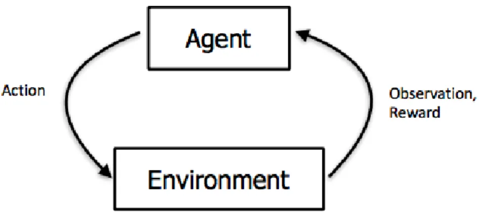
A typical RL model describes an agent taking actions in some environment and receiving rewards (typically scalar values) as a result (see Figure 1.1). The goal of the agent is to find best choice of actions for every given state such that agents returns (cumulative rewards) are maximized.

For example, in the classical game of Tic-Tac-Toe, the agent navigates 3×3

board states by choosing actions from a list of available cells, receiving +1 for a winning move (with −1to the opponent) and +0.5 for a tie.

There is no direct control over the specifics of the learned behavior, which are left for the agent to decide as long as it satisfies the goal of maximizing returns. This is in contrast with the more common Supervised Learning based approaches, where the researcher provides the agent with samples of state and optimal action pairs, typically collected by observing human experts.

Figure 1.1: Reinforcement Learning model of interaction with the environment.

Source: CS294 DRL Course, Berkeleyhttp://rll.berkeley.edu/deeprlcourse-fa15

Autonomy of learning agents in RL based approaches is the reason they are often considered to be closest to human intelligence and a potential key to eventually solving the problem of Artificial General Intelligence (AGI) – an AI capable of conscious thought and reasoning.

While the end goal of RL may lie in practical applications such as optimiza-tion of data center energy consumpoptimiza-tion [Gao, 2014] or even as grandiose as solving AGI, there is a need for simpler environments to initially test novel approaches. As the field evolved, games quickly became the benchmark environments of choice for many researchers as they are defined with (relatively) simple rules for navigation (ex. move up or down) and clear reward signals (ex. win or lose).

In fact, the birth of RL field is often linked to an early AI experiment with a self-learning agent that quickly surpassed its creator at the game of check-ers [Samuel, 1959]. This at the time monumental success for the AI field had the unfortunate side-effect of cultivating too much interest from the general public. The interest peaked with the release of Marvin Minsky’s “Perceptrons” book, but eventually lead to (understably) failed expectations and the so-called “AI winter”.

Problems of unreasonable expectations haunt the field of AI to this day, fueled now more so by fear of “Terminator”-like events, where a sentient AI chooses to eliminate the human race based on incorrectly provided reward function. It is important to consider the possibility of such events, and discuss ways to build in safety measures, but RL as a field is still in very early stages and it is more productive to focus on development and improvement of RL based approaches based on game environments.

Reinforcement Learning algorithms are often divided into based and model-free categories. Model-based algorithms attempt to learn a model of the envi-ronment, represented by the transition probabilities and reward function in the MDP formulation above. In contrast, model-free RL algorithms focus only on the end goal of cumulative reward maximization, effectively disregarding informa-tion about the environment the agent is operating in. While there are pros and cons to both approaches, RL researchers mainly focused on model-free algorithms due to their relative simplicity in implementation and computation. For simplic-ity, all the work that follows is implicitly assumed to be in the model-free RL family. The two dominant approaches to solving Reinforcement Learning problems in a model-free fashion are defined by the underlying optimization problem they are solving: either by optimizing on the expected value of the actions (e.g. Q-Learning) or on the policy itself (e.g. Policy Gradients). These approaches are different enough to have evolved into two separate families of algorithms and are explored in greater detail in sections 1.1.3, 1.1.4 below.

While there are many different approaches to solving RL based problems, one common thing between them all is in their mathematical formalization as a Markov Decision Process.

1.1.1

Markov Decision Process

The problem of RL can be viewed as a Markov Decision Process (MDP), which is formally defined by the < S, A, P, R > tuple:

• S: set of all possible states

• A: set of all possible actions

• P: (S, A, S)→[0,1], where P(s0|s, a) is the probability of arriving at s0 ∈S

given s∈S and a∈A

• R: (S, A, S)→_R, where R(s, a, s0)is the reward function for arriving in state

That is, given a set of all possible states S, a set of all possible actions A, transi-tion probability functransi-tionP, and a reward function R, find an optimal policy π – probability distribution over action space given current state – such that expected returns are maximized. Policy can be either deterministic π(s)or stochastic π(a|s).

The underlying stochastic process is defined by the transition probability P and in the context of RL problems (especially in games) is often implicitly assumed to be stationary, meaning it does not change over time. This assumption significantly simplifies following theoretical reasoning about the agent.

As the agent acts in the same environment with discrete timesteps, it is often useful to reason about the sequence of states, actions and rewards through time together as a single trajectory τ: < s0, a0, r1 >, < s1, a1, r2 >, . . . , < sn−1, an−1, rn>, where

rt represents agents immediate reward at a given time-stept: rt=R(st−1, at−1, st).

If full state information is not accessible to the agent then it is possible to ex-tend definition above and model the problem as a Partially Observable Markov Decision Process (POMDP), which defines an additional observation set O and its conditional probabilities PO(o|s0, a).

1.1.2

Credit Assignment Problem

While an agent receives some rewards immediately after an action was taken, it is often unclear whether the action actually contributed to the reward gained. Imagine a game of Tic-Tac-Toe where the agent has caught the opponent in a trap which will lead to his inevitable loss. While the win reward will be assigned to the final action, the contributing action was actually made beforehand. This is known as credit assignment problem and it is an open area of research.

One very common solution to the credit assignment problem is known as n-step discounted returns, where the cumulative rewards following action at for n steps

are exponentially weighted by some γ ∈(0,1]:

Rt = n

X

k=0

γkrt+k+1

The task is to then find an optimal policy π that maximizes expected returns

1.1.3

Value-Based Methods

In value-based RL methods the goal of finding an optimal policy π(s) is defined through maximizing the estimate the state value function:

Vπ(s) =Est+1∼P(·|st,at),at∼π(st)[Rt|st=s]

However, this task is not possible to solve in most real-world applications as we do not know the transition probabilities. For this reason the notion of state-action pair Qπ(s, a)(Q-value) is introduced and optimized instead:

Qπ(st, at) =Est+1∼P(·|st,at)[Rt|st=s, at =a]

Q-value represents expected cumulative reward given that action a∈A is taken in states∈S, followed by actions chosen based on the policyπ. It is often more useful to define Q-value recursively, separating immediate reward to its own component:

Qπ(st, at) = Est+1∼P(·|st,at)[R(st, at, st+1) +γQπ(st+1, at+1)]

Recursive definition above is commonly refered to as the Bellman Equation and is tightly related to the Bellman Optimality Equation:

Q∗(st, at) = Est+1∼P(·|st,at)[R(st, at, st+1) +γmax

at+1

Q∗(st+1, at+1)],

where Q∗(s, a)denotes an optimal state-action value function. This definition has a favorable property – it can be iteratively approximated (by e.g. bootstrapping). There are several algorithms based on this definition, one popular among them is the Q-Learning algorithm [Watkins and Dayan, 1992].

The Q-Learning algorithm approximates optimal state-action values Q∗(s, a) with Temporal Difference (TD) Learning, a general framework for iteratively optimizing a function while bootstrapping from current estimates [Sutton, 1988]. In context of Q-Learning, the TD update step is defined as follows (α is learning rate):

Qi+1(st, at)←Qi(st, at) +α rt+1+γmax

a Qi(st+1, a)−Qi(st, at)

This algorithm is guaranteed to produce an optimal greedy policyπ(s) = argmax

a

Q(s, a).

In practice, learned policy is often parametrized by some set of parameters θ. Though in that case convergence guarantees do not hold, empiricially this has proven not to be an issue in most RL based problems.

1.1.4

Policy-Based Methods

Alternative approach to value-based methods is to directly optimize the parametrized policyπ(a|s;θ)with regards to the expected returns_Est+1∼P(·|st,at),at∼π(st)[Rt|st= s].

There are several reasons why this approach could be beneficial or even the only viable option, for example continuous action space or a need for stochastic policy. In policy-based methods the optimization procedure is typically done with gradient descent family of algorithms. There are several ways to define the cost function for the underlying optimizer, but by far the most common method is the REINFORCE family [Williams, 1992].

The core of the REINFORCE approach is in its unbiased re-parametrization of the optimization target which results in their gradients definition being computa-tionally feasible for stochastic optimization procedure. Specifically, REINFORCE defines an unbiased estimate of ∇_θE[Rt|st] as∇θlogπ(at|st;θ)Rt [Williams, 1992].

1.1.5

Actor–Critic Methods

REINFORCE approach can be improved by reducing variance of the gradient estimate with a baseline bt(st) subtracted from the returns Rt, resulting in the

estimate ∇θE[Rt|st]taking the form ∇θlogπ(at|st;θ)(Rt−bt(st)), which is shown

to remain unbiased [Williams, 1992].

Often used baseline is an estimate of the state value function Vπ(s) =E[Rt|st= s].

Since Rt can be shown to be an estimate of Qπ(s, a) = E[Rt|st = s, at = a],

then Rt−Vπ(st) can be considered to be an estimate of the advantage function

A(st, at) =Qπ(st, at)−Vπ(st).

Algorithms that learn with the resulting estimate ∇θlogπst(at;θ) ˆA(st, at) are

referred to as the Actor-Critic methods, with the idea of the approach boiling down to the combination of optimization targets of the policy (actor) and the value (critic) terms [Sutton and Barto, 1998]. See Figure 1.2 below for a visual model.

Intuitively this approach can be understood as agents inner dialogue where the agent learns to act optimally in his environment, while scrutinizing his behavior based on the missed expected returns.

Though the critic terms name and its relation to Q-Learning can be deceiving, as critic’s task is not so much tied to agents ability to navigate the environment as it is to accurately predicting the value of the current state.

Figure 1.2: Actor-Critic model as illustrated in [Sutton and Barto, 1998].

1.2

Function Approximation

While an RL agent can be successfully trained on full state representations when the state space is relatively simple, the problem quickly becomes computationally infeasible as the state dimensionality and complexity grows. For this reason, a function approximator is often used that serves both as a dimensionality reduction technique and the mapping of similar states to the same result.

Though it should be noted that by using function approximators, convergence guarantees are not necessarily going to hold. In practice however that is rarely a significant problem. In particular, a staple of modern RL algorithms has become the use of a specific type of non-linear function approximators, commonly referred to as Artificial Neural Networks.

1.2.1

Artificial Neural Network

As the name suggests, Artificial Neural Networks are inspired by neuronal con-nections in the brain. The idea of using brain-inspired mathematical models was first explored relatively long ago [McCulloch and Pitts, 1943], but it only really took off with introduction of backpropagation: a method to iteratively calculate derivatives of complex functions by applying dynamic programming tech-niques [Rumelhart et al., 1986].

In practice, the backpropagation procedure is typically done behind the scenes by automatic differentiation libraries such as TensorFlow [Abadi et al., 2016] or PyTorch [Paszke et al., 2017].

Formally, ANNs can be viewed as non-linear function approximators:

ˆ

f(x) = Wnhn(Wn−1hn−1(. . .(W0x+b0). . .) +bn−1) +bn,

where hi(x) is the activation function – a function that ensures non-linearity in

the approximator at layer i. It was shown that with the correct choice of the activation function, ANNs are able to approximate any continuous function in a compact subset of _Rn_{, making them universal approximators [Hornik, 1991].}

Typical examples of h(x) are sigmoid and tanh.

Whilesigmoidandtanhwere favorable mathematically, having desirable properties such as continuity and differentiability, they also resulted in convergence break-ing side-effects such as “vanishbreak-ing” gradients, where the gradient of the function quickly became zero as the input grew in magnitude. Recently, Rectified Linear Unit (ReLU, h(x) = max(0, x)) became the nonlinearity function of choice for many researchers as it doesn’t suffer from vanishing gradient problems, and is computationally faster [Nair and Hinton, 2010].

ANNs enjoyed some success during 1980-1990, a notable example of that would be “ALVINN” - an automated vehicle where turning direction was chosen by the ANN [Pomerleau, 1989]. But their real potential was showcased only in second part of 2000s, when people started experimenting with running massively parallel matrix computations on specialized hardware, most notably on easily accessible consumer graphics processing units by NVIDIA.

This, coupled with practical advancements in model initialization [Hinton et al., 2006], led to breakthroughs in many areas. Notably, in 2012 this led to significant improve-ments over state-of-the-art at the time in speech recognition [Dahl et al., 2012] and in image recognition [Krizhevsky et al., 2012], the latter was done by making use of a special type of layer, specialized for spatial information processing – convolutional layer.

1.2.2

Convolutional Neural Network

Convolutional Neural Networks are a special type of ANN that contain one or more convolutional layers. These layers are designed to work well on certain types of

data such as images, making use of the inherent spatial information while keeping number of parameters relatively small (compared to classical ANNs). While used mainly for image processing, they have been recently shown to perform well on text-based tasks as well.

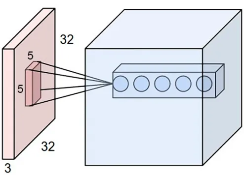
Each layer consists of a number of filters: small tensors, typically 3 ×3 ×C

or 5×5×C in size (where C matches the image depth), that produce outputs by performing sliding window dot products on localized parts of the input image step-by-step (Figure 1.3). Step size (or stride) is often fixed to 1 (meaning sliding window moves 1 pixel at a time), although other options are also not uncommon. Sometimes image dimensions will not be compatible with configured filter size and stride in which case input image border is often padded with zeros as a workaround. The idea of using convolutional layers on spatial information has been explored in the past [Fukushima, 1980], but the biggest showcase of their potential was probably done by “AlexNet” - a specialized ANN architecture that has won Ima-geNet Large Scale Visual Recognition Challenge in 2012 with a significant jump in classification accuracy performance [Krizhevsky et al., 2012]. This achievement is often referred to as the start of “Deep Learning” era in Machine Learning.

CNN based architectures are particularly notable because they are first examples of “end-to-end” solutions, where a single Artificial Neural Network performs all the necessary sub-tasks for problems such as recognition and classification. Prior to CNNs, typical image processing solutions contained multitude of hand-crafted filters and input preprocessing functions, all of which often required domain experts to write. Though some researchers argue that relying on convolutional layers in itself can be considered domain knowledge and thus CNN based approaches cannot be called truly “end-to-end”.

1.3

Deep Reinforcement Learning

Using Artificial Neural Networks as function approximators for classical RL al-gorithms has led to a significant improvement in their performance across many different tasks and environments. This has put the field of Reinforcement Learning into the spotlight both for researchers and the general public.

The idea itself was not novel and first successful applications date as far back as 1995 with TD-gammon: a Backgammon AI that relied on NNs for state eval-uation [Tesauro, 1995]. But the work that has led to bringing RL approaches notoriety is most likely to be DeepMind’s Atari AI.

Figure 1.3: Convolutional layer. Each circle represents a single filter of size5×5×3. Here the first filter is performing a dot product on the middle portion of the input image. Source: http://cs231n.github.io/convolutional-networks/

DeepMind researchers showed the full potential of RL based approaches with their Deep Q-Network paper, which used Atari Learning Environment – an emula-tor for the classical Atari console video games – as their benchmark environment. The importance of this paper was in the fact that the agent was learning to outplay human experts by learning only from the raw pixel inputs, not only resembling how a human would perceive the game, but also not having access to any domain knowledge from the experts [Mnih et al., 2015].

This was the first time an AI agent was capable of surpassing human perfor-mance in a complex environment while having no additional information such as domain specific features, and has led to an explosion in research of (Deep) Reinforcement Learning based approaches.

1.3.1

Advantage Actor-Critic (A2C)

The algorithm known as A2C has an interesting history of conception in that there is no official publication describing it, even though it is widely used and referenced.

In articles, A2C is often defined as a synchronous version of the Asynchronous Advantage Actor-Critic (A3C) algorithm [Mnih et al., 2016]. The two algorithms are essentially equivalent mathematically, though this is not the case when it comes to technical implementation.

Conceptually the A2C/A3C algorithms are quite similar to the classical actor-critic methods described in section 1.1.5, where the policyπs (actor) and value estimate

Vπ(s) (critic) are trained at the same time as a form of self-scrutinizing learning

loop. However, there are some key differences that are big enough to warrant considering them as a separate algorithm.

First, the use of Neural Networks as end-to-end non-linear function approximators both for the value and policy outputs. This breaks any convergence guarantees provided by the original algorithms, but significantly improves the level of com-plexity of environments an agent can learn to navigate in.

Second, the algorithms’ key selling point is in their capacity for mass parallelization. For A3C this is defined through client-server architecture, where each client contains a local copy of the model, computes its own gradients and pushes those to the central server. Central server performs a single optimization step based on the incoming gradients, updates model weights (parameters of the ANN) and then distributes new model version to all child workers.

In A2C, everything related to the model is stored on the server side, with client workers are only responsible for communicating with the environment itself. A2C workers are executed synchronously, which results in a trade-off between per-formance during sample gathering stage and during training stage. A2C gains significant computational speed due to the fact that the model can be efficiently executed on the GPU hardware, which is in contrast with the typically CPU only architecture of A3C based agents.

Finally, a common pitfall of the original actor-critic algorithms is the explo-ration/exploitation problem, which refers to maintaining a healthy balance between greedily following the current best policy (exploitation) and experimenting with alternative policies to see if the result improves (exploration). Since both policy and value functions are parametrized and are not guaranteed to converge to optimal values, an agent can quickly converge to some local optimum which may be far from desired behavior.

In the A2C/A3C algorithms this problem is alleviated by introducing a sepa-rate policy entropy maximization target to the gradient descend optimization objective. Specifically, the optimization problem is solved with the additional entropy term.

The full objective loss function for some sampled trajectory τ is defined as follows:

J(θ) = _Eτ logπ(at|st;θ) ˆA(st, at) + Rt−Vˆ(st;θ) 2 −π(at|st;θ) log(π(at|st;θ))

We can now present pseudo-code for the described Advantage Actor-Critic algorithm, roughly adapted from [Mnih et al., 2016]:

Algorithm 1 Advantage Actor-Critic algorithm

input: learning rateα, number of updatesTmax, number of n-steps tmax

while T < Tmax do:

t←0

Get s0 state

while t < tmax do:

Perform at∼π(·|st;θ)

Get rt reward and st+1 state

t←t+ 1

if st−1 is not terminal then:

Rtmax ←Vˆ(st−1;θ)

else

Rtmax ←0

for all i∈ {tmax−1, . . . ,0} do:

Ri ←ri+γRi+1

θ←θ+α∇θJ(θ)

T ←T + 1

1.4

StarCraft II

StarCraft was an immensely popular video game developed and published by Bliz-zard Entertainment in 1998. Much like the classical board games such as chess and go, StarCraft holds the property of being relatively easy to learn, but extremely difficult to master. This ensured that interest in the activity is not quickly lost and, given competitive nature of humans, eventually led to a competitive following.

Many consider StarCraft as one of the contributing games to the birth of the e-sports movement.

In fact, this game was considered a national sport of South Korea for almost two decades with many young people pursuing professional careers as StarCraft players, joining one of many organizations that specialized in this sport. Major tournaments were broadcasted live on television and gathered millions of viewers. Best players in South Korea were often very well-paid and recognized by the general public on same level as celebrities and athletes in more traditional sports.

However, given rapid technological advancement, StarCraft started to become out-dated and in 2010 Blizzard released its successor StarCraft II. While not as popular as its ancestor due to rise of many great competitors, it still gathers thousands of viewers for regular tournaments broadcasted live of various platforms.

The fact that this game is still played actively by millions of people across all levels of expertise from amateur beginner to professional veteran is very important from the point of view of AI research. Given that humans are still the best known solvers of complex and abstract tasks, they can play roles of a benchmarks for AIs and provide demostrations for the AI agents to learn from.

StarCraft II is a real-time strategy video game, which means that in order to win a player must continually make strategic decisions that are better than their adversary. A player starts with a set number of worker units and a central structure. Workers can either gather resources and return them to the central structure or, given enough resources, build additional structures. Central structure produces additional workers, but many others produce attacker type units which compose players army.

At any given time a player has access to only a small part of the game state. He has no direct access to what other players are doing, which contrast with most classical games and adds a significant layer of complexity to decision making. In order to win a player must “scout” his opponent by sending a unit to approximate position of opponents location and make educated guesses based on the (often minimal) information he has received before the scout was destroyed.

For simplicity of understanding, the game is often viewed in two distinct parts: “macro” and “micro”. Macro refers to general strategic and economic actions which may have long-term effects, such as choice of buildings and army composition. Micro refers to split-second decisions most often with regards to their army and

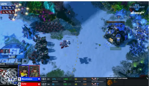
its actions towards opponents army or buildings. The ability to balance between making correct strategic decisions on a “macro” level mixed with controlling the army on a “micro” level is what often sets best players from others (Figure 1.4). Given that the game is real-time, a player must constantly make all the deci-sions, often multiple times per second. Number of decisions a player makes is measured by Actions Per Minute (APM) and for most professional players it is around 400, meaning a player makes about 6 actions every second throughout the game.

Additional complexity arises from the fact that each player can choose one of three district races, each with their own unique set of structures and units.

Figure 1.4: A game of StarCraft 2. Blue player must constantly switch between defending his resource gathering units from red player’s army and at the same time coordinating an attack of his own, seen on the minimap in bottom left. Source: Global StarCraft League tournament “GSL vs the World”, August 2017

Mathematically, StarCraft II can be viewed as POMDP (see section 1.1.1) with practically infinite state and action spaces. For this reason, it is especially beneficial to rely on function approximators when attempting to navigate this environment via RL based agents.

1.4.1

PySC2

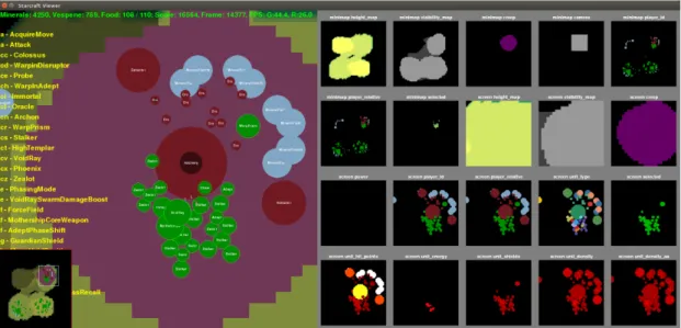
To communicate with the game programmatically, PySC2 library was used. This library exposes a list of spatial and non-spatial features containing information similar to what a player would have access to. All benchmark results were gathered on a set of minigames: maps with pre-defined sets of goals such as moving a unit to a target location, defeating enemy army or gathering resources and building structures (Figure 1.5). Full specification for input features and actions can be viewed online:

https://github.com/deepmind/pysc2/blob/master/docs/environment.md

Figure 1.5: PySC2 environment view example. On the left is a simplified game engine GUI meant to illustrate what is happening in the game for a human observer. On the right are the actual spatial features an AI agent would see, including unit and structure affiliation, types, health and visibility [Vinyals et al., 2017].

2. Agent for StarCraft II

In this chapter we first provide a birds-eye view of the implemented model archi-tecture. We then dive deeper into two key aspects: categorical feature embeddings and action policies with multiple outputs. These aspects are not only critical to the whole agent, but also neither present in other common benchmark environments such as Atari and MuJoCo, nor described in-depth in the reference publication. Finally, we describe some of the important implementation details such as platform choice and codebase structure.

2.1

Model Architecture

Agent model architecture closely follows FullyConv architecture description from the SC2LE paper and visualized in Figure 2.1 below. The name FullyConv refers to the fully convolutional, resolution preserving nature of the model, remaining spatial in structure from beginning to the end. This approach is in contrast with typical usages of convolutional layers, that reduce in size at each layer, ending with a conversion to a flat vector with dense layer on top (ex. Atari DQN architec-ture [Mnih et al., 2015]).

The need for spatial structure preserving architecture stems from the nature of the environment and how an agent typically interacts with it. A significant part of navigating StarCraft comes in the form of mouse clicks, either directly on the game screen or on the minimap. For this reason it would be beneficial for the spatial policies to remain in the same domain space as the incoming spatial features [Vinyals et al., 2017].

The model begins with three essentially separate blocks, representing different sources of information: two for spatial data (screen and minimap) and one for non-spatial data. First two sources represent the spatial data that an agent could see on the screen or on the minimap respectively (ex. unit type or health), whereas non-spatial data stands for additional information a player can get about the game state, such as number of resources or army count.

Spatial information inputs consist of n×n pixel “images”, where each pixel repre-sents value of the feature at a given pixel. Since most units are larger than a pixel in size, the information about them is duplicated across every pixel they occupy.

Spatial inputs are passed through two convolutional layers with 5 × 5, 3 ×3

size and 16, 32 filter count respectively. In order to preserve resolution, these layers have stride 1 and are evenly padded. Non-spatial inputs are logarithmically scaled and then broadcasted to the same dimensions as spatial inputs – that is, the information is repeated across every pixel in the image to match height and width of the spatial features.

The three blocks are then merged into a single H ×W ×D state representa-tion. From here the state is converted into a spatial policy, non-spatial policy and value estimate of the current state. Spatial policy conversion is done by applying one 1×1 convolutional layer with a single output filter. For non-spatial policy and value estimates the state is first pushed through a joint fully connected (FC) layer and then another final FC layer representing the policy and value estimate. A final softmax layer is applied to action policy outputs to obtain probability distributions. Action policies are described in greater detail in section 2.1.2.

Figure 2.1: FullyConv architecture as described and illustrated in [Vinyals et al., 2017].

2.1.1

Embedding Layer

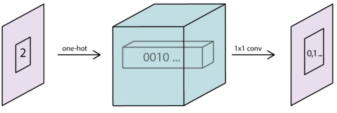
One special type of input information are the categorical spatial features, which represent some categorical data for every pixel in the feature “image”. For example, a unit could be represented byn×m pixel grid and every pixel in this grid would contain various information about this unit, such as its type (ex. marine, worker) or id of the player than controls him. As these features are not ordinal in nature, they can not be simply processed as is. One typical way to handle such situation is to apply one-hot expansion to a dimension that matches the number of categorical levels of the feature.

In case of spatial features naive one-hot expanding would be prohibitively ex-pensive from computational perspective. For example the unit type feature has over 1800 levels, which would result in a H×W ×1800sized tensor just on the input layer. For this reason, the one-hot expanded tensor must be reduced in the channel dimension back to a reasonable level (to continuous space in the SC2LE paper) with 1×1 convolutional layer (see Figure 2.2). Intuitively, this layer has a separate parameter responsible for recognizing different categorical levels of a given feature. Since input to the layer is a one-hot expanded tensor, an output will consist of an “image” where each pixel is filled with the relevant parameters value.

Figure 2.2: Embedding layer visualization. An input image ofH×W×1size with value 2 at a specified pixel is first one-hot expanded, producing an H×W ×C

tensor with all zeros except for 1 at index 2 for specified pixel’s vector. Resulting tensor is then passed through 1×1convolutional layer, arriving back to H×W×1

As the weights of the 1×1 convolutional layer are trained, a useful side-effect to the embedding layer emerges, similar to word2vec [Mikolov et al., 2013]. That is, the network learns to recognize the semantic similarity between different inputs such as two different units having similar role in the environment.

2.1.2

Action Policies

The action space provided by PySC2 environment is rich enough to express most, if not all, actions possible in a game as complex as StarCraft II. This includes left and right mouse clicks, boxed selection of units and queued actions (actions that are deferred until previous was completed).

At every timestep the environment provides an agent with a list of all possi-ble action identifiers their argument types. An example of a action identifier could be left-mouse click on the screen, which takes as argument coordinates of the click and whether the click is queued. For simplicity, we will refer to both action identifier and its argument choices as a single action step.

The most correct way to represent actions would be through their full joint proba-bility distribution, but such an approach would result in millions of possible values even for very low spatial dimensions, which would render any trainable approach virtually infeasible in the foreseeable future.

A simplifying assumption is made that action choices are conditionally independent from one another and are made entirely separately. This assumption of course does not hold in the real world (ex. argument type choices depend on their action identifier), but nonetheless works relatively well in practice.

Individual policy representations are obtained by either applying1×1convolutional layer or FC layer to the merged state representation for spatial and non-spatial policies respectively (preceding steps are described in detail in section 2.1). One final softmax layer is applied to convert model outputs to action probability distri-butions (Figure 2.3). Agent actions (both the indentifier and its arguments) are obtained by sampling the resulting probability distributions.

At any given point in time only a portion of actions are available to the agent, which is important to keep in mind when sampling the policies. For this reason a mask of available actions is applied one step before sampling, which effectively sets the probabilities of unavailable actions to zero. We then re-normalize the policy to ensure that the probabilities sum up to 1.

Figure 2.3: Action policy layer. State block is transformed into a spatial policy (used mainly for mouse-clicking on the screen) and non-spatial policy outputs. An output consist of probability distributions across possible values, such as action ids or specific pixels to click.

2.2

Implementation Details

Given that no official A2C paper was released, several sources of information were

pooled for inspiration during development of this agent: the original A3C [Mnih et al., 2016] paper, it’s GPU support extension paper G-A3C [Babaeizadeh et al., 2017], the

OpenAI baselines repository [Dhariwal et al., 2017] and PyTorch based RL al-gorithms repository [Kostrikov, 2018], both of which contained a reference A2C implementation. Earlier attempts to replicate SC2LE were also loosely referenced, however at the time of writing they were missing key aspects, relying on a different or incomplete architecture interpretation. Parts of the code that were most inspired by the attempts were marked with a reference link in the source code.

Agent is implemented with the Python programming language and TensorFlow – a general-purpose automatic differentiation library [Abadi et al., 2016]. With TensorFlow, complex differentiable layers can be defined seamlessly in a flexible computation graph. Derivatives of the layers are calculated automatically by applying the backpropagation algorithm. Additionally, NumPy [Oliphant, 2015] and SciPy [Jones et al., 01 ] were used for helper methods during input/output preprocessing stages.

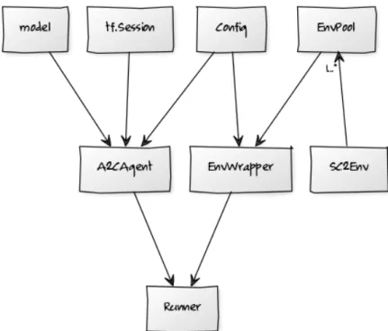
Agent codebase is designed with ease of extension in mind, either with alter-native algorithm implementations, model implementations or even with alteralter-native Starcraft II communication methods (such as the upcoming raw pixel API). See Figure 2.4 below for a visualization of the codebase structure.

Flexibility with regards to the choice of input features is key during experimentation step and lacking in alternative approaches. Here it is implemented as a list of accepted features stored in an external JSON configuration file which is loaded during initialization into aConfig class instance, passed toEnvPoolandA2CAgent instances.

Model-free algorithms such as A2C require significant amount of samples to learn even the most basic policies, which is why codebase was structured with strong support for parallelization. API is defined such that the number of environments is hidden away from the agent or its model, which means that any number of environments can be supported, only limited by hardware capabilities. This is for the most part enabled with strong vectorization capabilities of TensorFlow and NumPy.

Communication with the game engine is done through the SC2Env class from PySC2 library. Instances of SC2Env are created as separate processes and com-municated with via the EnvPool class, based on the feature specification loaded into the Config class. EnvPoolitself is wrapped with EnvWrapper which provides simple API for the agent to get relevant input features and provide necessary actions. The main class of the codebase is the A2CAgent, which accepts the TensorFlow Session instance,Configinstance and model definition as a lambda function defined in a separate class. This class is solely responsible both for acting and training of the agent. While having many responsibilities, content of the class was kept relatively short thanks to powerful vectorized operations support of TensorFlow.

The glue between the agent and the environment is implemented in a lightweight Runner class, which essentially only contains the main execution loop and logging utilities.

3. Evaluation

In this chapter we describe the different tasks (minigames) our agent is evaluated in, list the results the agent has obtained and provide commentary on how these results compare to the expectations and human expert benchmarks.

3.1

Tasks

Each evaluated task is a StarCraft II minigame: a map with some simple pre-defined MDP. These minigames are meant to test agents ability to learn and generalize across different environments.

MoveToBeacon map requires the agent to navigate a single unit to a beacon – a specific location on the map, identified by a large green circle.

In CollectMineralShards map the agent has to collect mineral shards (resource nodes) by walking on top of them. The map provides the agent with two units and an optimal strategy would be to navigate them simultaneously.

DefeatRoaches map introduces static opponent army units, which the agent has to defeat with his own. Opponent and agent units are significantly different, so the agent has to learn the characteristics of both types while only controlling its own units.

DefeatBanelingsAndZerglings map expands on the adversarial objective by providing opponent with two types of units: Zerglings and Banelings. The Baneling units can explode on contact with their opponents, meaning that the agent has to learn precise navigation and avoidance mechanisms in order to succeed.

FindAndDefeatZerglings map tests agents’ ability to navigate in a partially observable environment. An agent has to find and defeat opponent units scattered across the map.

CollectMineralsAndGas map objective is to test agents economic reasoning capabilities. The only goal of the map is to gather as many resources as possible, though there are multiple paths to achieving this goal, including building additional workers and a secondary base to speed up their gathering rate.

BuildMarines is similar to previous map, except the objective is to build as many units of a specific type (Marine) as possible. The path to building these units requires completion of multiple sub-tasks with long time-steps inbetween. This, in turn, tests agent’s long term planning capabilities.

3.2

Setup

Choice of hyperparameters such as learning rate, loss weights and batch size is typically made by repeatedly randomly sampling from some expected interval and training to a stable policy until satisfying results are achieved. Unfortunately this approach is not feasible for the StarCraft II environment as the agent might take sig-nificant amount of time before it is clear whether hyperparameter choice was good. Furthermore, even with fixed hyperparameters the end result varies wildly across dif-ferent seeds. For this reason many hyperparameters were chosen based on the initial performance of the agent on a subset of maps and locked for future experimentation. Screen and minimap resolution of presented results was locked to 16px for all map environments. For comparison, DeepMind used 64px resolutions. The choice for lower resolution is driven purely by time constraints, as computational require-ments grow significantly with higher resolutions (about 25x increase in wall clock time requirements for 64px). Agents capacity for learning in higher resolutions to the level of presented results was empirically verified at least once for every map. On some of the maps with higher resolution agents training speed improved in terms of number of samples required to reach the target results, but was unfortunately too slow in terms of wall clock time.

While the codebase was developed with dynamic configuration of input features in mind, they were locked across all map environments during results gathering phase to ensure that the agent is capable of generalizing – learning complex policies across varying environments.

Optimization algorithm was chosen between Adam [Kingma and Ba, 2014] and RMSProp [Tieleman and Hinton, 2012], two SGD improvements. RMSProp was used for all minigames exceptFindAndDefeatZerglings, where Adam was used in-stead. Adam is considered to be the best algorithm in supervised learning scenario, where its momentum build up helps jump through unfavorable local optima. For this same reason we have considered Adam to be unfavorable in RL scenarios as the input data distribution is inherently not stationary and thus momentum build up may be detrimental to agents performance. Surprisingly it has significantly

surpassed RMSProp on the FindAndDefeatZerglings minigame, perhaps due to the unique partially observable nature of the map.

All model weights were initialized with He initialization [He et al., 2015], which is shown to produce better results than the alternatives (eg. uniform or normal) and has become standard practice in modern Machine Learning.

3.3

Results

Results were collected by first training implemented agent until its average score matches baseline results and then executing in test mode, similarly to the training mode. The agent operates in 32 environments and the average score over those 32 runs is reported as the final result. If target score is not achieved in reasonable time then the training is prematurely terminated. Time limit depends on the minigame, from 30 minutes for MoveToBeacon to 50 hours for FindAndDefeatZerglings (wall clock time). To ensure that our agent is capable of converging to a policy with target results, we run training procedure four times with different random seeds. Results are summarized in the table 3.1 below.

Note that our method is different from how DeepMind has gathered their re-sults, where they launched 100 instances with different hyperparameter sets for 500 million frames and chose best out of them. This method was not chosen due to unrealistic computational requirements: obtaining results presented in this work took about 25,000 CPU hours in total, which means that repeating DeepMind experiments in full would take over 5,000,000 CPU hours.

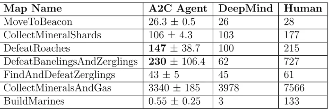
Map Name A2C Agent DeepMind Human

MoveToBeacon 26.3 ± 0.5 26 28 CollectMineralShards 106 ± 4.3 103 177 DefeatRoaches 147 ± 38.7 100 215 DefeatBanelingsAndZerglings 230 ± 106.4 62 727 FindAndDefeatZerglings 43 ±5 45 61 CollectMineralsAndGas 3340 ± 185 3978 7566 BuildMarines 0.55 ± 0.25 3 133

Table 3.1: Mean and std.dev of total reward for an episode of the implemented agents relative to DeepMind benchmarks. “A2C Agent” stands for our baseline im-plementation, “DeepMind” for DeepMind’s baseline FullyConv results and “Human” for DeepMind’s GradMaster ranked expert results.

3.4

Discussion

Our agent matches or slightly surpasses DeepMind FullyConv baseline results on most of the maps. A video of our agent navigating given set of maps has been recorded and available online: https://youtu.be/gEyBzcPU5-w

MoveToBeacon map can be considered solved, 2 point difference from human expert is most likely due to luck in random placements of the beacon. Specifically on this map the agent learned optimal policy very suddenly: behavior seemed quite random for majority of the time with optimal actions emerging almost instantly after first few good attempts.

CollectMineralShards map matches DeepMind baseline results, but is almost two times worse than human expert. The environment contains two units that could be controlled at almost the same time, singificantly increasing the speed of gathering the shards. Seems that the agent is unable to discover this strategy. DefeatRoaches map matches DeepMind baseline results, but is two times worse than human expert. Most likely optimal strategy is to defeat opponent army in parts by getting attention of a subset at a time.

DefeatBanelingsAndZerglings results are better than DeepMind’s baseline, but significantly worse than human benchmark. This map requires precise control of the individual units in the army in order to minimize damage from baneling explosions and the agent fails to learn anything more advanced than some initial splits. We observe significant variance of results in this minigame, most likely stemming from its volatile nature.

FindAndDefeatZerglings results match DeepMind baseline, but are worse than human expert. Most likely reason is that since the map is not fully visible, a human expert can remember where enemy army can be located on the map, whereas best policy our agent has discovered is to just move the units in a trajectory that covers the full map.

CollectMineralsAndGasresults are slightly below DeepMind baseline and more than two times worse than human expert. The "optimal" strategy our agent has learned is to simply send the initial workers to gather resources and wait for the remaining time. Judging by DeepMind results, their agents strategy is similar with maybe 1 more worker produced.

BuildMarines map proved to be too difficult for our agent to learn any rea-sonable policy on. Judging by relative score, this seems to be true for Deep-Mind agent as well. As this map requires long-term economic planning, solving it is most likely too difficult without some sort of temporal structure such as LSTM [Hochreiter and Schmidhuber, 1997].

3.4.1

Failures

In this section we list alternative choices (either architectural or in agent setup) that were considered failures due to agents poor performance.

Although the SC2LE paper only mentions embedding into continuous space, we have also experimented with having dimensionality reduced to a different space size. The size was either fixed to a small number (ex. 2 or 3) or dynamically changed based on the feature (ex. log₂(D), where D is number of categorical levels). In the end results were not consistently better than simply using continuous space. We have experimented with an alternative approach to embedding categorical spatial data described in section 2.1.1. While the main approach requires defining a separate embedding layer for every categorical feature, an alternative solution would be to combine all categorical spatial inputs into a single H×W × P

Ci

tensor, where Ci defines number of categorical levels of i-th feature. In theory this

approach had two benefits: ease of implementation and computation (can run a single convolutional operation for all categorical features at the same time) and the potential for learning interactions of different features since they all influenced each others output filters. However, empirically this lead to very unstable learning trajectory, often times oscillating between reasonable policies and borderline ran-dom behavior.

Singificant amount of time was spent investigating influence of various input features on agents speed of convergence to target results. While we have found some configurations that led to as much as 10x improvement in learning speed on some of the maps, they typically resulted in worse perfomance on other maps.

3.4.2

Future Work

Possible direction for future work could in investigating ways of improving sample efficiency of the agent (number of samples required to achieve target results), either by applying alternative algorithms such as PPO, ACKTR or SAC, or applying vari-ance reduction techniques from Monte Carlo methods such as Antithetic Variates.

A promising direction to explore would be to pre-train agent model in a supervised learning setting with data gathered from human experts.

An alternative direction could be in exploring Hierarchical Reinforcement Learning – a way to organize agents tasks into hierarchies. While the goal is to produce an agent capable of beating a professional human player in a modern video game such as StarCraft II, but solution to this task is still an open research question, potentially many years away.

Conclusion

We have investigated and implemented modern model-free Deep Reinforcement Learning algorithm: Advantage Actor Critic. We have measured its performance its ability to learn complex tasks, namely playing a modern video game with access to information similar to what a human player would have.

As a result, we have released an open-source implementation of the reference ANN based architecture described by DeepMind [Vinyals et al., 2017]. We have shown that our implementation is able to match reference results under mild game configuration simplifications to make the task feasible without access to expensive hardware.

Our open source implementation is available at https://github.com/inoryy/ pysc2-rl-agentand a video recording of the agent navigating reference tasks can be seen athttps://youtu.be/gEyBzcPU5-w.

Bibliography

[Abadi et al., 2016] Abadi, M., Barham, P., Chen, J., Chen, Z., Davis, A., Dean, J., Devin, M., Ghemawat, S., Irving, G., Isard, M., Kudlur, M., Levenberg, J., Monga, R., Moore, S., Murray, D. G., Steiner, B., Tucker, P., Vasudevan, V., Warden, P., Wicke, M., Yu, Y., and Zheng, X. (2016). TensorFlow: A system for large-scale machine learning. ArXiv e-prints.

[Babaeizadeh et al., 2017] Babaeizadeh, M., Frosio, I., Tyree, S., Clemons, J., and Kautz, J. (2017). Reinforcement learning thorugh asynchronous advantage actor-critic on a gpu. In ICLR.

[Dahl et al., 2012] Dahl, G. E., Yu, D., Deng, L., and Acero, A. (2012). Context-dependent pre-trained deep neural networks for large-vocabulary speech recogni-tion. IEEE Transactions on Audio, Speech, and Language Processing, 20(1):30–42. [Dhariwal et al., 2017] Dhariwal, P., Hesse, C., Klimov, O., Nichol, A., Plappert, M., Radford, A., Schulman, J., Sidor, S., and Wu, Y. (2017). Openai baselines. https://github.com/openai/baselines.

[Fukushima, 1980] Fukushima, K. (1980). Neocognitron: A self-organizing neural network model for a mechanism of pattern recognition unaffected by shift in position. Biological Cybernetics, 36(4):193–202.

[Gao, 2014] Gao, J. (2014). Machine learning applications for data center opti-mization.

[He et al., 2015] He, K., Zhang, X., Ren, S., and Sun, J. (2015). Delving deep into rectifiers: Surpassing human-level performance on ImageNet classification. In 2015 IEEE International Conference on Computer Vision (ICCV). IEEE. [Hinton et al., 2006] Hinton, G. E., Osindero, S., and Teh, Y.-W. (2006). A fast

learning algorithm for deep belief nets. Neural Computation, 18(7):1527–1554. [Hochreiter and Schmidhuber, 1997] Hochreiter, S. and Schmidhuber, J. (1997).

Long short-term memory. Neural Comput., 9(8):1735–1780.

[Hornik, 1991] Hornik, K. (1991). Approximation capabilities of multilayer feedfor-ward networks. Neural Networks, 4(2):251–257.

[Jones et al., 01 ] Jones, E., Oliphant, T., Peterson, P., et al. (2001–). SciPy: Open source scientific tools for Python. [Online; accessed <today>].

[Kempka et al., 2016] Kempka, M., Wydmuch, M., Runc, G., Toczek, J., and Jaskowski, W. (2016). ViZDoom: A doom-based AI research platform for visual reinforcement learning. In 2016 IEEE Conference on Computational Intelligence and Games (CIG). IEEE.

[Kingma and Ba, 2014] Kingma, D. P. and Ba, J. (2014). Adam: A Method for Stochastic Optimization. ArXiv e-prints.

[Kostrikov, 2018] Kostrikov, I. (2018). Pytorch implementations of re-inforcement learning algorithms. https://github.com/ikostrikov/ pytorch-a2c-ppo-acktr.

[Krizhevsky et al., 2012] Krizhevsky, A., Sutskever, I., and Hinton, G. E. (2012). Imagenet classification with deep convolutional neural networks. In Pereira, F., Burges, C. J. C., Bottou, L., and Weinberger, K. Q., editors, Advances in Neural Information Processing Systems 25, pages 1097–1105. Curran Associates, Inc. [McCulloch and Pitts, 1943] McCulloch, W. S. and Pitts, W. (1943). A logical

calculus of the ideas immanent in nervous activity. The Bulletin of Mathematical Biophysics, 5(4):115–133.

[Mikolov et al., 2013] Mikolov, T., Sutskever, I., Chen, K., Corrado, G. S., and Dean, J. (2013). Distributed representations of words and phrases and their compositionality. In Burges, C. J. C., Bottou, L., Welling, M., Ghahramani, Z., and Weinberger, K. Q., editors, Advances in Neural Information Processing Systems 26, pages 3111–3119. Curran Associates, Inc.

[Mnih et al., 2016] Mnih, V., Badia, A. P., Mirza, M., Graves, A., Lillicrap, T., Harley, T., Silver, D., and Kavukcuoglu, K. (2016). Asynchronous methods for deep reinforcement learning. In Balcan, M. F. and Weinberger, K. Q., editors, Proceedings of The 33rd International Conference on Machine Learning, volume 48 of Proceedings of Machine Learning Research, pages 1928–1937, New York, New York, USA. PMLR.

[Mnih et al., 2015] Mnih, V., Kavukcuoglu, K., Silver, D., Rusu, A. A., Veness, J., Bellemare, M. G., Graves, A., Riedmiller, M., Fidjeland, A. K., Ostrovski, G., Petersen, S., Beattie, C., Sadik, A., Antonoglou, I., King, H., Kumaran, D., Wierstra, D., Legg, S., and Hassabis, D. (2015). Human-level control through deep reinforcement learning. Nature, 518(7540):529–533.

[Nair and Hinton, 2010] Nair, V. and Hinton, G. E. (2010). Rectified linear units improve restricted boltzmann machines. In Proceedings of the 27th International Conference on International Conference on Machine Learning, ICML’10, pages

[Oliphant, 2015] Oliphant, T. E. (2015). Guide to NumPy. CreateSpace Indepen-dent Publishing Platform, USA, 2nd edition.

[Paszke et al., 2017] Paszke, A., Gross, S., Chintala, S., Chanan, G., Yang, E., DeVito, Z., Lin, Z., Desmaison, A., Antiga, L., and Lerer, A. (2017). Automatic differentiation in pytorch.

[Pomerleau, 1989] Pomerleau, D. A. (1989). Alvinn: An autonomous land vehicle in a neural network. In Touretzky, D. S., editor, Advances in Neural Information Processing Systems 1, pages 305–313. Morgan-Kaufmann.

[Rumelhart et al., 1986] Rumelhart, D. E., Hinton, G. E., and Williams, R. J. (1986). Learning representations by back-propagating errors. Nature,

323(6088):533–536.

[Samuel, 1959] Samuel, A. L. (1959). Some studies in machine learning using the game of checkers. IBM Journal of Research and Development, 3(3):210–229. [Silver et al., 2016] Silver, D., Huang, A., Maddison, C. J., Guez, A., Sifre, L.,

van den Driessche, G., Schrittwieser, J., Antonoglou, I., Panneershelvam, V., Lanctot, M., Dieleman, S., Grewe, D., Nham, J., Kalchbrenner, N., Sutskever, I., Lillicrap, T., Leach, M., Kavukcuoglu, K., Graepel, T., and Hassabis, D. (2016). Mastering the game of go with deep neural networks and tree search. Nature, 529(7587):484–489.

[Sutton, 1988] Sutton, R. S. (1988). Machine Learning, 3(1):9–44.

[Sutton and Barto, 1998] Sutton, R. S. and Barto, A. G. (1998). Introduction to Reinforcement Learning. MIT Press, Cambridge, MA, USA, 1st edition.

[Tesauro, 1995] Tesauro, G. (1995). Temporal difference learning and TD-gammon. Communications of the ACM, 38(3):58–68.

[Thorndike, 1898] Thorndike, E. (1898). SOME EXPERIMENTS ON ANIMAL INTELLIGENCE. Science, 7(181):818–824.

[Tieleman and Hinton, 2012] Tieleman, T. and Hinton, G. (2012). Lecture 6.5— RmsProp: Divide the gradient by a running average of its recent magnitude. COURSERA: Neural Networks for Machine Learning.

[van Seijen et al., 2017] van Seijen, H., Fatemi, M., Romoff, J., Laroche, R., Barnes, T., and Tsang, J. (2017). Hybrid Reward Architecture for Reinforcement Learning. ArXiv e-prints.

[Vinyals et al., 2017] Vinyals, O., Ewalds, T., Bartunov, S., Georgiev, P., Sasha Vezhnevets, A., Yeo, M., Makhzani, A., Küttler, H., Agapiou, J., Schrittwieser, J., Quan, J., Gaffney, S., Petersen, S., Simonyan, K., Schaul, T., van Hasselt, H., Silver, D., Lillicrap, T., Calderone, K., Keet, P., Brunasso, A., Lawrence, D., Ekermo, A., Repp, J., and Tsing, R. (2017). StarCraft II: A New Challenge for Reinforcement Learning. ArXiv e-prints.

[Watkins and Dayan, 1992] Watkins, C. J. C. H. and Dayan, P. (1992). Q-learning. Machine Learning, 8(3-4):279–292.

[Williams, 1992] Williams, R. J. (1992). Simple statistical gradient-following algo-rithms for connectionist reinforcement learning. Machine Learning, 8(3-4):229– 256.

Appendices

Source Code

Source code of the practical part of this thesis is available in a repository online on GitHub: https://github.com/inoryy/pysc2-rl-agent. This repository con-tains Python code of the agent that replicates [Vinyals et al., 2017] results, along with instructions to install and execute it locally.

Video Recordings

Two video recordings of the agent navigating described minigames are available: 1. With StarCraft II point of view: https://youtu.be/gEyBzcPU5-w

Licence

Non-exclusive licence to reproduce thesis and make thesis

public

I, Roman Ring,

1. herewith grant the University of Tartu a free permit (non-exclusive licence) to:

1.1 reproduce, for the purpose of preservation and making available to the public, including for addition to the DSpace digital archives until expiry of the term of validity of the copyright, and

1.2 make available to the public via the web environment of the University of Tartu, including via the DSpace digital archives until expiry of the term of validity of the copyright,

of my thesis

“Replicating DeepMind StarCraft II Reinforcement Learning Benchmark with Actor-Critic Methods”,

supervised by Ilya Kuzovkin and Tambet Matiisen.

2. I am aware of the fact that the author retains these rights.

3. I certify that granting the non-exclusive licence does not infringe the intel-lectual property rights or rights arising from the Personal Data Protection Act.