SFB
823
Robust discrimination
between long-range
dependence and a change
in mean
Discussion Paper
Carina Gerstenberger
Robust Discrimination between Long-Range
Dependence and a Change in Mean
Carina Gerstenberger
∗In this paper we introduce a robust to outliers Wilcoxon change-point testing procedure, for distinguishing between short-range dependent time series with a change in mean at un-known time and stationary long-range dependent time series. We establish the asymptotic distribution of the test statistic under the null hypothesis forL1 near epoch dependent
processes and show its consistency under the alternative. The Wilcoxon-type testing pro-cedure similarly as the CUSUM-type testing propro-cedure of Berkes, Horv´ath, Kokoszka and Shao (2006), requires estimation of the location of a possible change-point, and then using pre- and post-break subsamples to discriminate between short and long-range dependence. A simulation study examines the empirical size and power of the Wilcoxon-type testing procedure in standard cases and with disturbances by outliers. It shows that in standard cases the Wilcoxon-type testing procedure behaves equally well as the CUSUM-type testing procedure but outperforms it in presence of outliers.
KEYWORDS: Wilcoxon change-point test statistic; change-point; near epoch depen-dence; long-range dependence
1 Introduction
Since the pioneering work of Hurst (1951), Mandelbrot and Van Ness (1968) and Man-delbrot and Wallis (1968), the phenomenon of long-range dependence or Hust effect has been observed in many data sets, e.g. in hydrology, geophysics and economics. A lively debate also rages over the observed Hurst effect is due to long-range dependence or nonstationarity. Bhattacharya et al. (1983) showed that the Hurst effect detected by R/S statistics can be explained not only by long-range dependence, but by presence of a deterministic trend in short-range dependent data. Giraitis et al. (2001) showed that some modified R/S statistics reject the hypothesis of short-range dependence for long-range dependence but also for short-range dependent data in presence of a trend or change-points. The phenomenon of spurious long-range dependence has also been discussed in many other papers, see e.g. Granger and Hyung (2004).
A first attempt for distinguishing between long-range dependence and short-range de-pendence with a monotonic trend was made by K¨unsch (1986), who showed that the
Date: April 4, 2018.
periodogram in these two cases behaves differently. A test allowing to distinguish be-tween a stationary long-range dependent process and short-range dependent process with a change in mean was introduced by Berkes et al. (2006) and is based on the CUSUM statistic Cm,n(k) = k X i=m Xi− k−m+ 1 n n X i=1 Xi, m≤k≤n. (1)
It is well known that the CUSUM statistic is sensitive to outliers since it sums up the observations. In this paper we introduce a new robust to outliers testing procedure, which is based on the Wilcoxon change-point test statistic
Wm,n(k) = k X i=m n X j=k+1 (1{Xi≤Xj}−1/2), m≤k≤n. (2)
Dehling et al. (2013b, 2015) used this test statistic for testing for changes in the mean of long-range dependent and short-range dependent processes respectively. In both pa-pers the simulation studies point out that the Wilcoxon test statistic (2) is more robust to outliers than the CUSUM statistic (1). Recently, Gerstenberger (2018) showed that Wilcoxon-type change-point location estimator for a change in mean of short-range de-pendent data based on test statistic (2) is also robust against outliers.
The new Wilcoxon-type testing procedure suggested in this paper is based on the idea of Berkes et al. (2006). Firstly, given a sample X1, . . . , Xn, one estimates the location
ˆ
k of a possible change in mean. Then the test statistic is defined as the maximum of the Wilcoxon change-point statistic (2) applied to the subsamples X1, . . . , Xˆk and
Xkˆ+1, . . . , Xn.
Wilcoxon-type testing procedure
Assuming that sampleX1, . . . , Xn is given, we want to test the hypothesis
H0: Xi =Yi+µi, i= 1, . . . , n is generated by a stationary zero mean short-range
dependent process (Yj) and has a change in meanµ1 =. . .=µk∗ 6=µk∗+1 =. . .=µnat
unknown timek∗, against the alternative
H1: X1, . . . , Xn is a sample from a stationary long-range dependent process.
To construct the test statistic, first, we estimate the location k∗ of a change-point by a Wilcoxon-type change-point location estimator
ˆ k= minnk: max 1≤l<n W1,n(l) = W1,n(k) o , (3)
Next we divide the sample X1, . . . , Xn into subsamples X1, . . . , Xˆk and Xˆk+1, . . . , Xn, and set T(X1, . . . , Xn) =n−3/2 max 1≤k≤n W1,n(k) .
Then we computeT(X1, . . . , Xˆk) andT(Xˆk+1, . . . , Xn), and denote Tn,1:=T(X1, . . . , Xˆk) = ˆk−3/2 max 1≤k≤kˆ W1,ˆk(k) , (4) Tn,2 :=T(Xkˆ+1, . . . , Xn) = (n−ˆk)−3/2 max ˆ k<k≤n Wˆk+1,n(k) . (5)
Finally, we define the test statistic
Mn= max{Tn,1, Tn,2}. (6)
We show thatT(X1, . . . , Xn) allows to discriminate whether the sample has been
gener-ated by a short or long-range dependent stationary process. Hence, if we split the sample at time ˆk, which is close to the true change-pointk∗, since ˆk/k∗ →p 1 asymptotically we can assume that X1, . . . , Xˆk and Xkˆ+1, . . . , Xn are samples from a stationary sequence
with a constant mean, see Lemma 4.1 in Section 4. Subsequently, Mn can be used to
test if the samplesX1, . . . , Xˆk and Xˆk+1, . . . , Xn have been generated by a short-range
or long-range dependent stationary process.
The outline of the paper is as follows. Section 2 specifies assumptions allowing to es-tablish asymptotic distribution of Mn under H0 and consistency under H1. Section 3
compares finite sample performance of the Wilcoxon-type and the CUSUM-type testing procedure. All proofs are given in Section 4.
2 Definitions, assumptions and main results
In this section we present main assumptions, definitions and main results.
Throughout the paper,C denotes a generic non-negative constant, which may vary from time to time. The notation an ∼ bn means that sequences an and bn of real numbers
have property an/bn → c, as n → ∞, where c 6= 0. −→d and →p stand for convergence
in distribution and probability, respectively. By = we denote equality in distribution.d
kgk∞= supx|g(x)|denotes the supremum norm of a functiong.
Null hypothesis: short-range dependence with a change in mean
Under the null hypothesis we assume the random variablesX1, . . . , Xnfollow the
change-point model Xi = ( Yi+µ ,1≤i≤k∗ Yi+µ+ ∆n , k∗< i≤n, (7) where k∗ denotes the unknown location of the change-point in the mean and (Yj) is a
To cover a wide range of processes, we assume that the underlying process (Yj) can be
written asYj =f(Zj, Zj−1, Zj−2, . . .),j∈Z, wheref :RZ→Ris a measurable function,
and (Zj) is an absolutely regular (weakly dependent) process.
Definition 2.1. A stationary process (Zj) is called absolutely regular (or β-mixing) if βk= sup n≥1 E sup A∈Gn 1 P A|Gn∞+k −P (A)→0, (8) as k→ ∞, where Gm
k is the σ-field generated by random variablesZk, . . . , Zm, k < m.
Absolute regularity orβ-mixing implies the weaker property ofα-mixing, see e.g. Bradley (2007).
In addition, we will assume that (Yj) satisfies near epoch dependence condition, i.e. Yj
depends on the near past of (Zj).
Definition 2.2. A stationary process (Yj) is L1 near epoch dependent (L1 NED) on
some stationary process (Zj) with approximation constants ak,k≥0, if
E|Y1−E(Y1|G−kk)| ≤ak, k= 0,1,2, . . . (9)
where Gk
−k is the σ-field generated by random variables Z−k, . . . , Zk and ak → 0 as
k→ ∞.
Notice that a linear process or AR process might not be absolutely regular, but it would beL1near epoch dependent; see Example 2.1 in Gerstenberger (2018) for linear processes
and Hansen (1991) for GARCH(1,1) processes. More examples ofL1 NED processes can
be found in Borovkova et al. (2001), who also discuss more generalLr NED processes, r≥1.
We need further additional assumptions on the distribution functionF ofY1, the mixing
coefficients βk in (8) andak in (9).
Assumption 1. The process (Yj) in (7) is L1 NED on some absolutely regular process
(Zj) with mixing coefficients βk and approximation constantsak such that
∞ X k=1 k2(βk+ √ ak)<∞. (10)
Moreover, Y1 has a continuous distribution function F with bounded second derivative,
and variables Y1−Yk, k≥1 satisfy
P(x≤Y1−Yk ≤y)≤C|y−x|, (11) for allx≤y, where C does not depend on k andx, y.
We suppose that both, the unknown change-point k∗ and the magnitude of change ∆n
Assumption 2. a) The change-point k∗ = [nθ], where 0 < θ < 1 is fixed, is propor-tional to the sample size n.
b) The magnitude of change ∆n in (7) depends on n, and is such that
∆n→0, n∆2n→ ∞, n→ ∞.
An important step of our testing procedure is the estimation of the location k∗ of the change-point in mean. Gerstenberger (2018) showed that under Assumptions 1 and 2 the Wilcoxon-type change-point location estimator ˆk in (3) is consistent,
∆2nkˆ−k∗
=OP(1), asn→ ∞. (12)
Alternative: long-range dependence
Under alternative H1, the sample X1, . . . , Xn is generated by a stationary long-range
dependent process:
Xi=G(ξi) +µ, i= 1, . . . , n, (13)
where µ is the unknown mean and (ξj) is a stationary long memory Gaussian process
with E(ξ1) = 0,Var(ξ1) = 1 and (non-summable) auto-covariancesγk = Cov(ξ1, ξ1+k)∼ k2d−1c
0, where c0 >0 and d∈ (0,1/2). Furthermore, we assume that G :R → R is a
measurable, strictly monotone function such that E(G(ξ1)) = 0.
Main results
The following theorem derives the limit distribution of the test procedure under the null hypothesisH0. Below,B(t) =W(t)−tW(1) denotes a standard Brownian bridge, where
W(t) is a standard Brownian motion.
Theorem 2.1. Let (Xj) follow the model in (7). Then, under Assumptions 1 and 2, Mn= max{Tn,1, Tn,2}−→d σmax n sup 0≤t≤1 B(1)(t) , sup 0≤t≤1 B(2)(t) o =:σZ (14)
where B(1) and B(2) are two independent Brownian bridges, σ2 =
∞
X
k=−∞
Cov (F(Y0), F(Yk)), (15)
and F denotes the distribution function of Y1.
Since the limit distribution ofMn depends on the long-run varianceσ2, to calculate the
critical values for the test, we need to estimate the long-run variance; see Section 3. We will compare performance of our test with the CUSUM-type test by Berkes et al.
(2006) defined as ˜
where ˜ TC(X1, . . . , Xn) = (ˆsn √ n)−1 max 1≤k≤n C1,n(k) ,
is based on the CUSUM statistic C1,n(k) in (1). ˜kC = min n k : max1≤l≤n C1,n(l) = C1,n(k) o
is a CUSUM-type estimator of k∗ and ˆs2n is a long-run variance estimator of
σc2 = P∞
k=−∞Cov (Y0, Yk) given in (21). Berkes et al. (2006) showed that under their
assumptions under the null hypothesis, ˜MC,n d
− →Z.
The next theorem establishes consistency of the test Mn, i.e. that the test will detect
long-range dependence with probability tending to 1.
Theorem 2.2. Let (Xj) be as in (13). Then, as n→ ∞, Mn→p∞.
Proofs of Theorem 2.1 and 2.2 are given in Section 4.
3 Simulation Study
In this simulation study we compare the finite sample performance (size and power) of the Wilcoxon-type testing procedureMnin (6) with the CUSUM-type testing procedure
˜
MC,n of Berkes et al. (2006), given in (16).
Simulation set up
To calculate the empirical size we generate the sample of random variables X1, . . . , Xn
using the change-point model
Xi= (
Yi+µ ,1≤i≤k∗
Yi+µ+ ∆ , k∗ < i≤n,
(17)
whereYi =ρYi−1+i is an AR(1) process withρ= 0.4 and standard normal innovations i. We setk∗ = [nθ],θ= 0.25,0.5,0.75 and ∆ = 0.5,1,2.
To evaluate theempirical power of the test we generate a sampleX1, . . . , Xnof fractional
Gaussian noise (fGn)
Xi=WH(i+ 1)−WH(i), (18)
where WH(t), H = d+ 1/2 ∈ (1/2,1) is a fractional Brownian motion, see e.g.
Man-delbrot and Van Ness (1968). The sequence (Xj) is a long-range dependent process:
Cov(X1, X1+k)∼k2d−1c0 with long-range dependence parameterd∈(0,1/2). We
con-siderd= 0.1,0.2,0.3,0.4.
To analyse the robustness of Wilcoxon and CUSUM testing procedures to outliers, we replace observationsX[0.2n], X[0.4n], X[0.6n], X[0.8n]in the sample (X1, . . . , Xn) (under the
We consider sample sizesn= 200,500,1000,2000,5000. All simulation results are based on 10,000 replications.
Critical values
To analyse the empirical size and power, we need to know the critical values for the tests
Mn and ˜MC,n.
By Theorem 2.1, under the null hypothesis,
Mn= max Tn,1, Tn,2 d − →σZ.
Hence, if ˆσ2(X1, . . . , Xk) is a consistent estimator for the long-run varianceσ2 based on
the sample X1, . . . , Xk, then
ˆ Mn= max n Tn,1 ˆ σ(X1, . . . , Xˆk) , Tn,2 ˆ σ(Xˆk+1, . . . , Xn) o d − →Z.
The same asymptotics holds for the CUSUM test: ˜MC,n d
−
→Z, see Corollary 2.1 of Berkes
et al. (2006). Thus, the critical value cα for a given significance level α is obtained by
solving
P Z > cα
=α. (19)
Since B(1) and B(2) are independent Brownian bridges, (19) reduces to P sup 0≤t≤1 B(1)(t) ≤cα = (1−α)1/2, (20) where sup0≤t≤1B(1)(t)
has the well-known Kolmogorov-Smirnov distribution, and its
quantiles can be found in statistical tables. Forα= 5% (20) implies c5%= 1.478.
Estimation of long-run variance
The selection of a long-run variance estimate ˆσ in ˆMn has a strong impact on the size
and power properties of the tests in finite samples. To estimate the long-run varianceσ2c =P∞
k=−∞Cov (Y0, Yk) in ˜MC,n in (16), Berkeset al.(2006) suggested to use the Bartlett estimator
ˆ s2n= 1 n n X i=1 Xi−X¯n 2 + 2 q(n) X j=1 1− j q+ 1 1 n n−j X i=1 Xi−X¯n Xi+j−X¯n , (21)
where ¯Xn =n−1Pni=1Xi, with the bandwidth q(n) = Clog10(n). Table 1 reports the
empirical size (for θ = 0.5, ∆ = 1) and power (for d= 0.4) in % at significance level 5% of ˜MC,n test, with ˆs2n as in (21) computed with bandwidth 15 log10(n). It shows
n = 500 1000 2000 5000 emp. size 0.05 0.87 2.48 3.79 power 0.30 7.62 27.44 60.51
Table 1: Empirical size and power of ˜MC,n test using the Bartlett estimator.
alternative, which has also been pointed out by Baek and Pipiras (2012) and Preuß et al.(2017).
In our simulation study to improve the performance of ˜MC,n test we proceed as follows.
To estimateσ2
C, instead of ˆs2n, we use the non-overlapping subsampling estimator of σC2
by Carlstein (1986), with block length ln,
ˆ σ2C = 1 [n/ln] [n/ln] X i=1 1 ln iln X j=(i−1)ln+1 Xj− ln n n X j=1 Xj 2 , (22)
which yields better size and power balance for ˜MC,n, as seen from Tables 2 and 4. This
estimator has also been used by Dehlinget al.(2015) for a CUSUM-type test for changes in the mean of a short-range dependent process.
In turn, for our test ˆMn to estimate σ we shall use the Carlstein type estimator for
long-run variance proposed by Dehling et al. (2013a),
ˆ σW = 1 [n/ln] r π 2 [n/ln] X i=1 1 √ ln iln X j=(i−1)ln+1 Fn(Xj)− ln n n X j=1 Fn(Xj) , (23)
whereFn(x) =n−1Pni=11{Xi≤x}. Note that ˆσW estimatesσ, notσ 2.
The Carlstein estimator ˆσC2 as well as the estimator ˆσW (23) are subsampling type
estimators and require to choose a suitable block length ln. The choice ofln is widely
discussed in the literature. For AR(1)-processes Carlstein (1986) suggests to use
ln= max
n1/3(2ρ/(1−ρ2))2/3
,1 , (24)
whereρ denotes the autocorrelation coefficient at lag 1. In our simulation study we use this block length with ρ estimated by the sample autocorrelation coefficient ˆρ since it yields good results for the empirical size and power.
In the presence of outliers, we need to robustify further the choice of the block length. Since the sample autocorrelation is highly sensitive to outliers, we use in (24) a robust estimator ofρ proposed by Ma and Genton (2000),
ˆ
ρQ=
Q2n−1(u+v)−Q2n−1(u−v)
Q2n−1(u+v) +Q2n−1(u−v), whereQn= 2.21914{|Xi−Xj|;i < j}(k), which is the k= n2
/4-th order statistic of the
n
2
Frequency 0.0 0.1 0.2 0.3 0.4 0 1000 2000 3000 4000
(a) sample autocorrelation
Frequency 0.20 0.25 0.30 0.35 0.40 0.45 0.50 0.55 0 500 1000 1500 (b) MG-estimator
Figure 1: Histogram of ˆρ(1) and ˆρQ(1) based on 10,000 replications. Xi is generated by
an AR(1) process with outliers,i ∼N(0,1),ρ= 0.4 and n= 500.
(1993), u = (X1, . . . , Xn−1) and v = (X2, . . . , Xn). Figure 1 contains the histogram of
estimates ˆρ and ˆρQ based on 10,000 replications of sample X1, . . . , X500 with outliers,
generated by an AR(1) model with ρ= 0.4 and i.i.d. standard normal innovations. For a further discussion on robust estimation of autocorrelation function see D¨urre et al.
(2015).
Simulation results
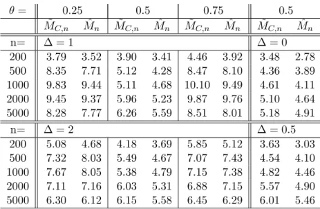
Table 2 reports the empirical size at the 5% significance level based on 10,000 replications of ˜MC,nand ˆMntests, for the model (17) without outliers. The empirical size of ˆMnand
˜
MC,n slightly exceed the 5% level for large sample size n forθ = 0.5 and ∆ = 0.5,1,2.
The size of the tests is more distorted if the change-point is located close to the beginning or end of the sample, i.e. forθ= 0.25,0.75. We also consider the situation of no change, i.e. ∆ = 0, for which the empirical size of both testing procedures is close to the nominal size. Empirical sizes of ˆMn and ˜MC,n are comparable in the absence of outliers.
Table 3 reports the empirical size of ˆMn and ˜MC,n in presence of outliers. While test
ˆ
Mn is robust to the outliers, the test ˜MC,n becomes too conservative.
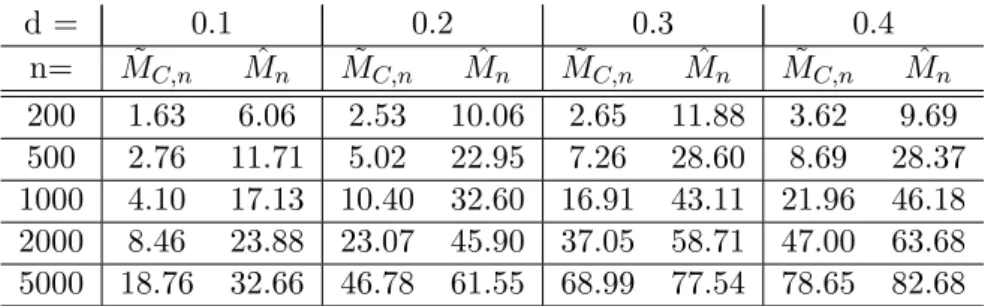
Tables 4 and 5 report the empirical power of test ˜MC,n and ˆMn, forXi in (18) without
outliers and with outliers, respectively. Table 4 shows that the power of both tests increases with increasing sample size and dependence parameter d(except power of ˆMn
for n= 200, d= 0.4). It shows that in absence of outliers ˆMn and ˜MC,n have similar
power properties.
Table 5 shows that the empirical size of ˆMn is practically not affected by the outliers,
whereas ˜MC,n suffers a loss of power.
Since the nominator of the CUSUM-type test is based on partial sums, outliers in the data have strong impact on the test statistic ˜MC,n and hence, one should expect that
it over rejects the true hypothesis H0. Since presence of outliers increases the
θ= 0.25 0.5 0.75 0.5 ˜ MC,n Mˆn M˜C,n Mˆn M˜C,n Mˆn M˜C,n Mˆn n= ∆ = 1 ∆ = 0 200 3.79 3.52 3.90 3.41 4.46 3.92 3.48 2.78 500 8.35 7.71 5.12 4.28 8.47 8.10 4.36 3.89 1000 9.83 9.44 5.11 4.68 10.10 9.49 4.61 4.11 2000 9.45 9.37 5.96 5.23 9.87 9.76 5.10 4.64 5000 8.28 7.77 6.26 5.59 8.51 8.01 5.18 4.91 n= ∆ = 2 ∆ = 0.5 200 5.08 4.68 4.18 3.69 5.85 5.12 3.63 3.03 500 7.32 8.03 5.49 4.67 7.07 7.43 4.54 4.10 1000 7.67 8.05 5.38 4.79 7.15 7.38 4.82 4.46 2000 7.11 7.16 6.03 5.31 6.88 7.15 5.57 4.90 5000 6.30 6.12 6.15 5.58 6.45 6.29 6.01 5.46
Table 2: Empirical size of ˜MC,n and ˆMn tests at the 5% significance level, 10,000
repli-cations. Xi follows the model (17) without outliers.
θ= 0.5 ˜ MC,n Mˆn M˜C,n Mˆn n= ∆ = 1 ∆ = 2 200 1.21 3.21 0.60 3.61 500 0.92 4.30 0.56 4.64 1000 0.86 4.72 0.62 4.77 2000 1.35 5.31 0.94 5.26 5000 2.67 5.71 1.95 5.58
Table 3: Empirical size of ˜MC,n and ˆMn tests at the 5% significance level, 10,000
repli-cations. Xi follows the model (17) with outliers.
d = 0.1 0.2 0.3 0.4 n= M˜C,n Mˆn M˜C,n Mˆn M˜C,n Mˆn M˜C,n Mˆn 200 7.68 5.90 12.28 9.99 14.11 11.50 12.53 9.35 500 14.12 11.53 25.31 22.84 31.52 28.33 32.03 28.42 1000 20.22 16.95 35.37 32.64 46.41 43.11 50.22 46.06 2000 26.67 23.90 49.17 45.95 61.92 58.68 67.50 63.52 5000 35.05 32.68 64.44 61.27 79.67 77.48 85.12 82.63
Table 4: Empirical power of ˜MC,n and ˆMn tests at the 5% significance level, 10,000
d = 0.1 0.2 0.3 0.4 n= M˜C,n Mˆn M˜C,n Mˆn M˜C,n Mˆn M˜C,n Mˆn 200 1.63 6.06 2.53 10.06 2.65 11.88 3.62 9.69 500 2.76 11.71 5.02 22.95 7.26 28.60 8.69 28.37 1000 4.10 17.13 10.40 32.60 16.91 43.11 21.96 46.18 2000 8.46 23.88 23.07 45.90 37.05 58.71 47.00 63.68 5000 18.76 32.66 46.78 61.55 68.99 77.54 78.65 82.68
Table 5: Empirical power of ˜MC,n and ˆMn tests at the 5% significance level, 10,000
replications. Xi follows the model (18) with outliers.
reduction of size and a loss in power.
In general, we conclude that Wilcoxon test ˆMnallows discrimination between long-range
dependence and short-range dependence with a change in mean that is robust to outliers. In absence of outliers it performs equally well as CUSUM test ˜MC,n, but outperforms it
in presence of outliers.
4 Proofs
This section contains the proofs of Theorem 2.1, Theorem 2.2 and auxiliary lemmas. 4.1 Proof of Theorem 2.1
Suppose thatX1, . . . , Xn follow the model in (7) and Assumptions 1 and 2 are satisfied.
Throughout the proofs without loss of generality, we assumeµ= 0 and ∆n>0.
Proof of Theorem 2.1. We divide the proof into two steps, as in the proof of Theorem 2.1 in Berkeset al. (2006).
First, in Lemma 4.1 below we show that with ˆkas in (3),
Tn(X1, . . . , Xˆk) =Tn(Y1, . . . , Yˆk) +oP(1)
and
Tn(Xˆk+1, . . . , Xn) =Tn(Ykˆ+1, . . . , Yn) +oP(1).
Subsequently, in Lemma 4.2 below we prove that
Tn(Y1, . . . , Yˆk), Tn(Yˆk+1, . . . , Yn)
d
−
→σ(Z(1), Z(2)),
whereZ(i) = sup0≤t≤1|B(i)(t)|,i= 1,2. Then, the claim (14) of Theorem 2.1 follows by the continuous mapping theorem.
Before proceeding to Lemma 4.1, similarly to the notationWm,n(k) in (2), we define Um,n(k) = k X i=m n X j=k+1 (1{Yi≤Yj}−1/2), m≤k≤n. (25)
Lemma 4.1. Let X1, . . . , Xn follow the model in (7), and Assumptions 1 and 2 be satisfied. Let kˆ be defined as in (3). Then,
n−3/2 max 1≤k≤ˆk W1,ˆk(k) =n−3/2 max 1≤k≤ˆk U1,kˆ(k) +oP(1) (26) n−3/2 max ˆ k<k≤n Wˆ k+1,n(k) =n−3/2 max ˆ k<k≤n Uˆ k+1,n(k) +oP(1). (27)
Proof. We have to distinguish between two cases, ˆk≤k∗ and ˆk > k∗, wherek∗ = [nθ]. If ˆk≤k∗, then by (7), Xi =Yi,i= 1, . . . ,kˆ, and hence,W1,ˆk(k) =U1,kˆ(k),k= 1, . . . ,kˆ.
In turn, Xi = Yi for i = ˆk+ 1, . . . , k∗, and Xi =Yi+ ∆n fori = k∗+ 1, . . . , n. Since
1{Yi+∆n≤Yj+∆n} = 1{Yi≤Yj},Wˆk+1,n(k) can be decomposed into two terms,
Wkˆ+1,n(k) = ( Ukˆ+1,n(k) + Pk i=ˆk+1 Pn j=k∗+11{Yj<Yi≤Yj+∆n}, k < kˆ ≤k∗ Ukˆ+1,n(k) +Pk ∗ i=ˆk+1 Pn j=k+11{Yj<Yi≤Yj+∆n}, k ∗< k≤n.
If ˆk > k∗, similar argument yields, Wkˆ+1,n(k) =Uˆk+1,n(k), fork= ˆk+ 1, . . . , n and
W1,ˆk(k) = ( U1,ˆk(k) +Pki=1P ˆ k j=k∗+11{Yj<Yi≤Yj+∆n}, 1≤k≤k ∗ U1,ˆk(k) + Pk∗ i=1 Pˆk j=k+11{Yj<Yi≤Yj+∆n}, k ∗ < k≤ˆk. (28)
Proof of (26). For ˆk ≤ k∗, equation (26) holds trivially, since W1,ˆk(k) = U1,kˆ(k), k =
1, . . . ,kˆ.
For ˆk > k∗, equation (28) yields,
W1,ˆk(k)−U1,kˆ(k) ≤ k∗ X i=1 ˆ k X j=k∗+1 1{Yj<Yi≤Yj+∆n} =:I1,ˆk(k ∗),
for all 1≤k≤ˆk. Hence, using Lemma 4.3i),
n −3/2 max 1≤k≤ˆk W1,ˆk(k) −n−3/2 max 1≤k≤ˆk U1,kˆ(k) ≤n −3/2I 1,ˆk(k ∗).
Thus, property (26) holds ifn−3/2I1,ˆk(k∗) =oP(1).
By Lemma 4.5 below, n−3/2I1,kˆ(k∗) = n−3/2k∗(ˆk−k∗)Θ∆n +oP(1), where Θ∆n =
E 1{Y0
2<Y10≤Y20+∆n}
andY10 andY20 are independent copies of Y1. The distribution
func-tion F ofY1 has bounded second derivative. Hence, asn→ ∞,
Θ∆n = E 1{Y20<Y10≤Y20+∆n} = P Y 0 2 < Y 0 1 ≤Y 0 2+ ∆n = Z R (F(y+ ∆n)−F(y))dF(y) = ∆n Z R f2(y)dy+o(1) . (29)
Furthermore, by (12), ∆2n|ˆk−k∗|=OP(1) and by Assumption 2,k∗/n∼θand n∆2n→ ∞, asn→ ∞. This yields n−3/2k∗|kˆ−k∗|Θ∆n ≤C ∆2nkˆ−k∗ n1/2∆ n =oP(1).
This completes the proof of (26). The proof of (27) follows using similar argument.
Lemma 4.2. Let (Yj) satisfy Assumption 1 and let Assumption 2 hold. Then, T(Y1, . . . , Ykˆ), T(Ykˆ+1, . . . , Yn) d − →σ sup 0≤t≤1 B(1)(t) , σ sup 0≤t≤1 B(2)(t) , (30)
where B(1) and B(2) are independent Brownian bridges, and σ is given in (15).
Proof. To prove Lemma 4.2 we will use the idea of the proof of Theorem 3 of Dehling
et al. (2015).
Recall that T(Y1, . . . , Ykˆ) = ˆk−3/2max1≤k≤kˆ|U1,ˆk(k)| and similarly T(Yˆk+1, . . . , Yn) =
(n−ˆk)−3/2maxk<kˆ ≤n|Uˆk+1,n(k)|. Note that the terms U1,ˆk(k) andUˆk+1,n(k) defined in
(25) can be written as a second order U-statistic
Ua,b(k) = k X i=a b X j=k+1 (h(Yi, Yj)−Θ), a≤k < b,
with kernel function h(x, y) = 1{x≤y} and constant Θ = Eh(Y10, Y20) = 1/2, where Y10
and Y20 are independent copies ofY1.
By applying Hoeffding’s decomposition of U-statistics to Ua,b(k), the kernel function h
can be written as the sum
h(x, y) = Θ +h1(x) +h2(y) +g(x, y), (31) whereh1(x) = Eh(x, Y20)−Θ = 1/2−F(x), h2(y) = Eh Y10, y −Θ =F(y)−1/2, g(x, y) =h(x, y)−h1(x)−h2(y)−Θ. Therefore, Ua,b(k) = k X i=a b X j=k+1 (h1(Yi) +h2(Yj) +g(Yi, Yj)) =:sa,b(k) +va,b(k), where sa,b(k) = (b−k) k X i=a h1(Yi) + (k−a+ 1) b X j=k+1 h2(Yj), va,b(k) = k X i=a b X j=k+1 g(Yi, Yj).
Note that va,b(k) = k X i=1 b X j=1 g(Yi, Yj)− k X i=1 k X j=1 g(Yi, Yj)− a−1 X i=1 b X j=1 g(Yi, Yj) + a−1 X i=1 k X j=1 g(Yi, Yj).
Thus, Lemma 4.4 below yields
n−3/2 max a≤k≤b va,b(k) ≤4n−3/2 max 1≤k≤n1max≤l≤n k X i=1 l X j=1 g(Yi, Yj) =oP(1).
Furthermore, by Lemma 4.3 ii), max a≤k≤b Ua,b(k) = max a≤k≤b sa,b(k) + max a≤k≤b va,b(k) = max a≤k≤b sa,b(k) +oP(n3/2).
It remains to show that ˆ k−3/2 max 1≤k≤ˆk s1,kˆ(k) d − →σ sup 0≤t≤1 B(1)(t) , (n−ˆk)−3/2 max ˆ k<k≤n sˆk+1,n(k) d − →σ sup 0≤t≤1 B(2)(t) ,
whereB(1)andB(2)are independent Brownian bridges. By Slutsky’s Lemma this implies (30). Note that h1(x) =−h2(x). Hence,
s1,ˆk(k) = (ˆk−k) k X i=1 h1(Yi) +k ˆ k X j=k+1 h2(Yj) = ˆkn1/2 n 1 n1/2 k X i=1 h1(Yi)− k ˆ k 1 n1/2 ˆ k X i=1 h1(Yi) o =: ˆkn1/2Γ(1)k and sˆk+1,n(k) = (n−k) k X i=ˆk+1 h1(Yi) + (k−ˆk) n X j=k+1 h1(Yj) = (n−ˆk)n1/2 n 1 n1/2 k X i=ˆk+1 h1(Yi)− k−ˆk n−ˆk 1 n1/2 n X i=ˆk+1 h1(Yi) o = (n−ˆk)n1/2n 1 n1/2 Xk i=1 h1(Yi)− ˆ k X i=1 h1(Yi) −k−kˆ n−ˆk 1 n1/2 Xn i=1 h1(Yi)− ˆ k X i=1 h1(Yi) o =: (n−kˆ)n1/2Γ(2)k .
Corollary 4.1 below implies convergence of finite dimensional distribution of the partial sum process, 1 n1/2 [nt] X i=1 h1(Yi) 0≤t≤1 d − →(σW(t))0≤t≤1,
whereW(t) is a Brownian motion andσ as in (15). By the Skorokhod-Wichura-Dudley representation (see e.g., Shorack and Wellner (2009), Theorem 4 on page 47) there exists a series of Brownian motionsWn(t),t∈[0,1], such that
sup 0≤t≤1 n −1/2 [nt] X i=1 h1(Yi)−σWn(t) =oP (1). Set Γ(1)W,k =Wn k n −k ˆ kWn kˆ n , Γ(2)W,k=Wn k n −Wn kˆ n −k−kˆ n−ˆk Wn(1)−Wn ˆk n . Thus, max 1≤k≤ˆk Γ (1) k −σΓ (1) W,k =oP(1), max ˆ k<k≤n Γ (2) k −σΓ (2) W,k =oP(1).
Consistency of ˆkin (12), ∆2n|ˆk−k|=OP(1), and Assumption 2,n∆2n→ ∞, as n→ ∞,
yield ˆ k n−θ =oP(1).
Therefore, by the continuity of Brownian motionWnand using the continuous mapping
theorem,Wn ˆk/n −Wn(θ) =oP(1). Hence, max 1≤k≤kˆ Γ (1) W,k = sup 0≤t≤θ Wn(t)− t θWn(θ) +oP (1) and max ˆ k<k≤n Γ (2) W,k = sup θ<t≤1 Wn(t)−Wn(θ) − t−θ 1−θ Wn(1)−Wn(θ) +oP(1) d = sup θ<t≤1 Wn(t−θ)− t−θ 1−θWn(1−θ) ,
since Brownian motions have stationary increments and Wn(0) = 0. Finally,
(ˆk/n)−1/2 max 1≤k≤ˆk Γ (1) k = σ θ1/2 sup 0≤t≤θ Wn(t)− t θWn(θ) +oP(1) d =σ sup 0≤t≤1 B(1)(t) ,
since Brownian motions are scale invariant, i.e. θ−1/2W
n(t) d =Wn(t/θ), and ((n−kˆ)/n)−1/2 max ˆ k<k≤n Γ (2) k d = σ (1−θ)1/2 θ<tsup≤1 Wn(t−θ)− t−θ 1−θWn(1−θ) d = σ (1−θ)1/2 0<tsup≤1−θ Wn(t)− t 1−θWn(1−θ) d =σ sup 0≤t≤1 B(2)(t) .
The increments of Brownian motions are independent, thusB(1) and B(2) are indepen-dent. This proves the lemma.
Concept of 1-continuity
Before we state the auxiliary results, we recall the concept of 1-continuity, which was introduced by Borovkovaet al. (2001).
To study the asymptotic behaviour of the Wilcoxon test
W1,n(k) = k X i=1 n X j=k+1 (1{Xi≤Xj}−1/2)
we need to show that the function h(x, y) = 1{x≤y} is 1-continuous. Then the variables
(h(Yi, Yj)) retain some characteristics of the variables (Yi, Yj).
Definition 4.1. (Borovkova et al. (2001))
We say that the kernelh(x, y)is1-continuous with respect to a distribution of a station-ary process(Yj) if there exists a functionφ(), ≥0 such that φ()→0, →0, and for all >0 and k≥1 E h(Y1, Yk)−h Y10, Yk 1{|Y 1−Y10|≤} ≤φ(), (32) Eh(Yk, Y1)−h Yk, Y10 1{|Y 1−Y10|≤} ≤φ(), and E h Y1, Y20 −h Y10, Y201{|Y 1−Y10|≤} ≤φ(), (33) Eh Y20, Y1 −h Y20, Y10 1{|Y 1−Y10|≤} ≤φ(),
where Y20 is an independent copy ofY1 and Y10 is any random variable that has the same
distribution asY1.
For a univariate functiong(x), the 1-continuity property is defined as follows.
Definition 4.2. The function g(x) is 1-continuous with respect to a distribution of a stationary process (Yj) if there exists a functionφ(), ≥0 such thatφ()→0, →0, and for all >0
Eg(Y1)−g Y10 1{|Y 1−Y10|≤} ≤φ(), (34)
where Y10 is any random variable that has the same distribution as Y1.
The following remark states functionsh(x, y) = 1{x≤y},h1(x),h2(x) andg(x, y)
appear-ing in the Hoeffdappear-ing decomposition (31) are 1-continuous functions.
Remark 4.1. Let (Yj) be a stationary process, Y1 has continuous distribution function
i) The functionh(x, y) = 1{x≤y} is 1-continuous function (i.e. satisfies (32) and (33))
with respect to the distribution of (Yj) with function φ() =C, for some C > 0,
see e.g. Corollary 4.1 of Gerstenberger (2018).
ii) Lemma 2.15 of Borovkova et al. (2001) yields that if a general function h(x, y) satisfies (32) and (33) with some function φ() then Eh(x, Y20), where Y20 is an independent copy ofY1, satisfies the condition in (34) with the same functionφ().
Hence,h1(x) = Eh(x, Y20)−1/2 andh2(x) = Eh(Y20, y)−1/2 are 1-continuous.
iii) The function g(x, y) =h(x, y)−h1(x)−h2(x)−1/2 is 1-continuous (satisfies (32)
and (33)), sincehandh1satisfy (32), (33) and (34) withφ() =C, for someC >0.
In particular, E|g(Y1, Yk)−g(Y10, Yk)|1{|Y1−Y10|≤} ≤E |h(Y1, Yk)−h(Y10, Yk)|1{|Y1−Y0 1|≤} + E |h1(Y1)−h1(Y10)|1{|Y1−Y10|≤} ≤2φ() and similarly, E |g(Yk, Y1)−g(Yk, Y10)|1{|Y1−Y10|≤} ≤2φ(). Auxiliary results
The following lemma yields maximum inequalities used in the proofs of Lemma 4.1 and Lemma 4.2.
Lemma 4.3. Let(ak)and(bk)be two sequences of real numbers andck=ak+bk. Then, i) maxk|ak| −maxk|bk|
≤maxk|ak−bk|
ii) maxk|ak| −maxk|bk| ≤maxk|ck| ≤maxk|ak|+ maxk|bk|.
Proof. We start with the proof of i). Assume that maxk|ak| ≥ maxk|bk| and define
˜
k= arg maxk|ak|. Note that |b˜k| ≤maxk|bk|. Then, max k |ak| −maxk |bk| = max k |ak| −maxk |bk| ≤ |ak˜| − |b˜k| ≤ |a˜k| − |b˜k| ≤ |ak˜−b˜k| ≤max k |ak−bk|.
For maxk|ak| ≤maxk|bk|the proof follows a similar argument using ˜k= arg maxk|bk|. Proof of ii). It is obvious that maxk|ck|= maxk|ak+bk| ≤maxk|ak|+ maxk|bk|. Define
˜
k= arg maxk|ak|. Then
max
k |ak+bk| ≥maxk (|ak| − |bk|)≥ |a˜k| − |b˜k| ≥maxk |ak| −maxk |bk|,
The following lemma derives the functional central limit theorem for partial sum pro-cesses of (h1(Yj)).
Corollary 4.1. Suppose that the assumptions of Lemma 4.2 hold. Then, 1 n1/2 [nt] X i=1 h1(Yi) 0≤t≤1 d − →(σW(t))0≤t≤1,
where W (t) is a Brownian motion and σ is given in (15).
Proof. Wooldridge and White (1988) in Corollary 3.2 established a functional central limit theorem for partial sum process Pk
i=1Y˜i, k ≥ 1, for a process ( ˜Yj) which is L2
NED on a strongly mixing process ( ˜Zj). Therefore, Corollary 4.1 is proved, by showing
that (h1(Yj)) isL2 NED on a strongly mixing process.
By Proposition 2.11 of Borovkova et al. (2001), if (Yj) is L1 NED on a stationary
absolutely regular process (Zj) with approximation constantsakandg(x) is 1-continuous
with functionφ, then (g(Yj)) is alsoL1 NED on (Zj) with approximation constantsa0k= φ √2ak
+ 2√2ak||g||∞. By Remark 4.1 ii),h1(x) = 1/2−F(x) is 1-continuous function
withφ() =C. Thus, the processes (h1(Yj)) is L1 NED processes with approximation
constantsa0k=C√ak≥φ
√
2ak
+ 2√2ak||h1||∞.
Observe that the variables ηk :=h1(Y1)−E(h1(Y1)|G−kk) satisfy the L1 NED condition
(9) with a0k. To show L2 NED for (h1(Yj)) note that by definition of h1, Eh1(Y1) = 0
and |h1(Y1)| ≤C <∞. Thus,
Eηk2≤E|ηk| ·(|h1(Y1)|+|E(h1(Y1)|G−kk)|)
≤CE|ηk| ≤Ca0k.
The last inequality holds, because byL1 NED of (h1(Yj)), E|h1(Y1)−E(h1(Y1)|G−kk)| ≤ a0k. Therefore, the process (h1(Yj)) is alsoL2NED on (Zj) with approximation constant a0k=Ca1k/2. Moreover, absolute regularity of (Zj) implies the process (Zj) is also strong
mixing. Assumption (10) yields a0k = O(k−1/2) and βk = O(k−2). Thus, (h1(Yj))
satisfies the conditions of Corollary 3.2 of Wooldridge and White (1988) which implies
1 n1/2 [nt] X i=1 h1(Yi) 0≤t≤1 d − →(σW(t))0≤t≤1,
whereW (t) is a Brownian motion andσ2 =P∞
k=−∞Cov(F(Y1), F(Yk)).
Next we show that the contribution of g(x, y) of the Hoeffding decomposition (31) is negligible.
Lemma 4.4. Suppose that the assumptions of Lemma 4.2 hold. Then, n−3/2 max 1≤k≤n1max≤l≤n k X i=1 l X j=1 g(Yi, Yj) =oP(1). (35)
Proof. We first prove for 1≤q ≤p≤n, 1≤h≤l≤n, E n −3/2 p X i=q+1 l X j=h+1 g(Yi, Yj) 2 ≤ C n3(p−q)(l−h). (36)
Proof of (36) Lemma 1 of Dehling et al. (2015) showed if f is a 1-continuous bounded degenerate kernel function andφf() satisfies
∞ X k=1 k(β(k) +√ak+φf(ak))<∞, (37) then E k X i=1 n X j=k+1 f(Yi, Yj) 2 ≤Ck(n−k), 1≤k≤n. (38)
The proof of Lemma 1 in Dehlinget al.(2015) shows that (38) can be extended to (36). Hence, to complete the proof, we need to verify thatg(x, y) satisfies the assumptions of Lemma 1 of Dehlinget al. (2015).
By the Hoeffding decomposition (31), g(x, y) =h(x, y) +F(x)−F(y)−1/2. Note that EF(Y1) = 1/2, thus Eg(x, Y1) = Eg(Y1, y) = 0, i.e. g(x, y) is a degenerate kernel.
Furthermore, g(x, y) is bounded, since h(x, y) = 1{x≤y} and F(x) are bounded. By
Remark 4.1 iii) g(x, y) is 1-continuous with φ() =C, the latter satisfies (37) because of condition (10). This completes the proof of (36).
Proof of (35)To prove the lemma, we use Theorem 10.2 of Billingsley (1999), which states that if the increments of partial sumsSi =Pij=1ζi of random variablesζi,i= 1,2, . . .
are bounded in probability, in particular if there exist α > 1, β > 0 and non-negative numbersun,1, . . . , un,n such that
P |Sj−Si| ≥ ≤ 1 β j X l=i+1 un,l α ,
for >0, 0≤i≤j≤n, then for all >0,n≥2,
P max 1≤k≤n|Sk| ≥ ≤ K β n X l=1 un,l α ,
whereK >0 depends only on α andβ. Denote Gn(l) =n−3/2 max 1≤k≤n k X i=1 l X j=1 g(Yi, Yj) ,
withGn(0) = 0 and define random variables ζi=Gn(i)−Gn(i−1), whereζ0 = 0. Note
thatSi =Pij=1ζi =Gn(i) and by Lemma 4.3 i)for 1≤h≤l≤n,
P (|Sl−Sh| ≥)≤P n−3/2 max 1≤k≤n k X i=1 l X j=1 g(Yi, Yj)− k X i=1 h X j=1 g(Yi, Yj) ≥ = P n−3/2 max 1≤k≤n k X i=1 l X j=h+1 g(Yi, Yj) ≥ .
Let us now define
˜ Sk= k X i=1 n−3/2 l X j=h+1 g(Yi, Yj) .
Note that for 1≤q≤p≤n,
S˜p−S˜q =n−3/2 p X i=q+1 l X j=h+1 g(Yi, Yj) .
By Markov inequality and (36),
P S˜p−S˜q ≥ ≤ 1 2 E S˜p−S˜q 2 ≤ 1 2 C n3(p−q)(l−h)≤ 1 2 Xp t=q+1 un,t 4/3 , where un,t= C 3/4
n9/4(l−h). Hence, ˜Si satisfies assumption of Theorem 10.2 of Billingsley
(1999) withβ = 2,α= 4/3. Thus, for any fixed >0,
P max 1≤k≤n S˜k ≥ ≤ K 2 n X t=1 C3/4 n9/4(l−h) 4/3 ≤ 1 2 (l−h)C 3/4 n5/4 4/3 and moreover P (|Sl−Sh| ≥)≤P max 1≤k≤n S˜k ≥ ≤ 1 2 l X t=h+1 un,t 4/3 , where un,t = C 3/4
n5/4. Therefore, Si satisfies assumption of Theorem 10.2 of Billingsley
(1999) withβ = 2,α= 4/3. Finally, for any fixed >0, asn→ ∞,
Pn−3/2 max 1≤l≤n1max≤k≤n k X i=1 l X j=1 g(Yi, Yj) ≥ = P max 1≤l≤n Sl ≥ ≤ K 2 n X t=1 C3/4 n5/4 4/3 ≤ K 2 1 n1/3 →0,
In the following we state auxiliary results to deal with the terms ˜ U1,ˆk(k∗) := k∗ X i=1 ˆ k X j=k∗+1 1{Yj<Yi≤Yj+∆n}, ˆk≥k ∗, and ˜ Ukˆ+1,n(k∗) := k∗ X i=ˆk+1 n X j=k∗+1 1{Yj<Yi≤Yj+∆n}, ˆk < k ∗
appearing in the proof of Lemma 4.1.
Note that the terms ˜U1,ˆk(k∗) and ˜Ukˆ+1,n(k∗) can be written as a second order U-statistic
˜ Ua,b(k) = k X i=a b X j=k+1 hn(Yi, Yj), a≤k < b,
with kernel function hn(x, y) = 1{y<x≤y+∆n}.
Applying Hoeffding’s decomposition of U-statistics (Hoeffding (1948)) to ˜Ua,b(k),
de-composes the kernel functionhn into the sum
hn(x, y) = Θ∆n+h1,n(x) +h2,n(y) +gn(x, y), (39) with Θ∆n= E 1{Y20<Y10≤Y20+∆n} , h1,n(x) = Ehn x, Y20 −Θ∆n =F(x)−F(x−∆n)−Θ∆n, h2,n(y) = Ehn Y10, y −Θ∆n =F(y+ ∆n)−F(y)−Θ∆n, gn(x, y) =hn(x, y)−h1,n(x)−h2,n(y)−Θ∆n,
whereY10 and Y20 are independent copies ofY1.
Lemma 4.5. Suppose that the assumptions of Lemma 4.1 hold. Then, n−3/2 U˜1,ˆk(k ∗ )−k∗(ˆk−k∗)Θ∆n =oP(1) (40) and n−3/2 ˜ Uˆk+1,n(k∗)−(k∗−ˆk)(n−k∗)Θ∆n =oP(1), (41) where Θ∆n = E 1{Y20<Y10≤Y20+∆n}
andY10 and Y20 are independent copies of Y1 .
Proof. Let us start with the proof of (40). The Hoeffding decomposition (39) yields
˜ U1,kˆ(k∗)−k∗(ˆk−k∗)Θ∆n = k∗ X i=1 ˆ k X j=k∗+1 (h1,n(Yi) +h2,n(Yj) +gn(Yi, Yj)) = (ˆk−k∗) k∗ X i=1 h1,n(Yi) +k∗ ˆ k X j=k∗+1 h2,n(Yj) + k∗ X i=1 ˆ k X j=k∗+1 gn(Yi, Yj).
Therefore, n−3/2 U˜1,ˆk(k ∗ )−k∗(ˆk−k∗)Θ∆n ≤n−3/2 (ˆk−k ∗) k∗ X i=1 h1,n(Yi) +k∗ ˆ k X j=k∗+1 h2,n(Yj) +n −3/2 k∗ X i=1 ˆ k X j=k∗+1 gn(Yi, Yj) .
Note that the indicator function hn(x, y) = 1{y<x≤y+∆n} is bounded. Furthermore, by
(29), Θ∆n ∼C∆n, thus
|h1,n(x)| ≤ |F(x)−F(x−∆n)−Θ∆n| ≤C∆n+ Θ∆n ≤C∆n, (42)
|h2,n(x)| ≤ |F(x+ ∆n)−F(x)−Θ∆n| ≤C∆n+ Θ∆n ≤C∆n,
where C > 0 is a constant. Hence, gn(x, y) = hn(x, y)−h1,n(x) −h2,n(y)−Θ∆n
is bounded. Since Eh1,n(Y1) = 0 and Eh2,n(Y1) = 0, gn(x, y) is a degenerate kernel,
i.e. Egn(x, Y1) = Egn(Y1, y) = 0. hn(x, y) satisfies (32) and (33) with φhn() = C,
see e.g. Corollary 4.1 of Gerstenberger (2018). Then, with similar argument as in Remark 4.1,h1,n and h2,n are 1-continuous and therefore, gn(x, y) is 1-continuous with
function φgn() =Csatisfying (37). Hence, gn(x, y) satisfies the conditions on g(x, y)
in Lemma 4.4, which yields
n−3/2 k∗ X i=1 ˆ k X j=k∗+1 gn(Yi, Yj) ≤2 max1≤k≤n1max≤k≤nn −3/2 k X i=1 l X j=1 gn(Yi, Yj) =oP(1).
Thus, it remains to shown−3/2(ˆk−k∗)
Pk∗ i=1h1,n(Yi) +k∗P ˆ k j=k∗+1h2,n(Yj) =oP(1).
By (42), we receive the following inequality
n−3/2 (ˆk−k ∗ ) k∗ X i=1 h1,n(Yi) +k∗ ˆ k X j=k∗+1 h2,n(Yj) ≤n−3/2C(ˆk−k∗)k∗∆n=C k∗ n ∆2n|ˆk−k∗| n1/2∆ n =oP(1),
where we used the consistency of ˆk in (12), ∆2
n|ˆk−k∗| = OP(1), and Assumption 2, k∗/n∼θand n∆2n→ ∞as n→ ∞. This completes the proof of (40).
The proof of (41) follows using similar argument. 4.2 Proof of Theorem 2.2
Under the alternative we consider observations X1, . . . , Xn with Xi = G(ξi) +µ, i =
1, . . . , n. Note that the indicator function 1{x≤y} is invariant under strictly increasing
decreasing function, observe that 1{G(ξi)≤G(ξj)} = 1−1{ξi≤ξj}. Therefore, for G being strictly monotone, k X i=1 n X j=k+1 (1{Xi≤Xj}−1/2) = k X i=1 n X j=k+1 (1{ξi≤ξj}−1/2) .
Thus, to prove Theorem 2.2 it is sufficient to considerTn,1 andTn,2 in (4), (5) applied to
the stationary Gaussian process (ξj), i.e. Tn,1(ξ1, . . . , ξkˆ) andTn,2(ξˆk+1, . . . , ξn), instead
of Tn,1(X1, . . . , Xkˆ) and Tn,2(Xˆk+1, . . . , Xn).
Before we prove that the test Mn tends to infinity in probability under the
alterna-tive, we will consider the limit distribution of Tn,1(ξ1, . . . , ξˆk) and Tn,2(ξˆk+1, . . . , ξn) in
Lemma 4.7, using a different normalization nd+3/2cd, where c2d =
c0
d(2d+1),c0 >0. Note
that in the following we always assumed∈(0,1/2). By (WH(t))0≤t≤1 we denote a
frac-tional Brownian motion process with Hurst parameterH=d+ 1/2, that is a mean zero Gaussian process with auto-covariances Cov(WH(t), WH(s)) = (t2H+s2H− |t−s|2H)/2.
Lemma 4.6. Assume that the assumptions of Theorem2.2 hold. Then, for0≤s≤t≤
1, 1 nd+3/2c d [ns] X i=1 n X j=[nt]+1 (1{ξi≤ξj}−1/2) d − → 1 2√π s(WH(1)−WH(t))−(1−t)WH(s) ,
where WH,H =d+ 1/2 is a standard fractional Brownian motion, c2d=
c0
d(2d+1), c0 >0
and d∈(0,1/2).
In the proof of Lemma 4.6 we apply the empirical process non-central limit theorem of Dehling and Taqqu (1989), which uses the Hermite expansion of 1{G(ξ)≤x}−F(x).
Before proceeding to the proof, we will have a brief look at this concept.
Hermite expansion: Since function g(ξ) = 1{G(ξ)≤x}−F(x) is a measurable function
with Eg(ξ) = 0 and Eg2(ξ) <∞, ξ ∼N(0,1), i.e. g∈ L2(
R, N), we could represent g
by its Hermite expansion
g(ξ) = ∞ X i=1 Jk(x) k! Hk(ξ),
where the equality means convergence in theL2 sense. Thek-th order Hermite
polyno-mial is given by Hk(ξ) = (−1)keξ 2/2 dk dξke −ξ2/2 ,
and the coefficients are given byJk(x) = E(1{G(ξ)≤x}Hk(ξ)), withJ1(x) = E(ξ11{ξ1≤x}) =
−ϕ(x), where ϕ(x) denotes the standard normal density function. The Hermite rank is defined as m = min{k≥0 :Jk 6= 0}, the smallest k for which the term in the Hermite
Hermite process: The limit processZm(t) in Theorem 1.1 of Dehling and Taqqu (1989)
is calledm-th order Hermite process and is defined e.g. in Taqqu (1978). Ifm= 1,Z1(t)
is the standard Gaussian fractional Brownian motion.
Proof of Lemma 4.6. Dehling et al. (2013b) have shown in their Theorem 1 that
1 nd+3/2c d [ns] X i=1 n X j=[ns]+1 (1{Xi≤Xj}−1/2) 0≤s≤1 d − → 1 m!(Zm(s)−sZm(1)) Z R Jm(x)dF(x) 0≤s≤1
for Xi =G(ξi), where G :R→ R is a measurable function (that might not be strictly
monotone), F is the continuous distribution of Xi, m is the Hermite rank of the class
functions 1{G(ξi)≤x}−F(x), andJm(x),Hm and (Zm(s))s∈[0,1] are given above.
Following the proof of Theorem 1 of Dehlinget al. (2013b) we will show
1 nd+3/2c d [ns] X i=1 n X j=[nt]+1 (1{Xi≤Xj}−1/2) 0≤s≤t≤1 d − → 1 m! (1−t)Zm(s)−s(Zm(1)−Zm(t) Z R Jm(x)dF(x) 0≤s≤t≤1 . (43)
Since F is a continuous distribution function, R
RF(x)dF(x) = 1/2. Denote Fk(x) = 1 k Pk i=11{Xi≤x} and Fk+1,n(x) = 1 n−k Pn i=k+11{Xi≤x}. Then, [ns] X i=1 n X j=[nt]+1 (1{Xi≤Xj}−1/2) = [ns](n−[nt]) Z R F[ns](x)−F(x) dF[nt]+1,n(x) + [ns](n−[nt]) Z R F(x)d F[nt]+1,n−F (x).
Integration by parts yields,
Z R F(x)d F[nt]+1,n−F (x) =− Z R F[nt]+1,n−F (x)dF(x). Hence, [ns] X i=1 n X j=[nt]+1 (1{Xi≤Xj}−1/2) = [ns](n−[nt]) Z R (F[ns](x)−F(x))dF[nt]+1,n(x) −[ns](n−[nt]) Z R (F[nt]+1,n(x)−F(x))dF(x).
With the same argument as used in Dehling et al. (2013b), we show that [ns](n−[nt]) nd+3/2c d Z R (F[ns](x)−F(x))dF[nt]+1,n(x)− (1−t) m! Z R Jm(x)Zm(s)dF(x)→0 (44) [ns](n−[nt]) nd+3/2c d Z R (F[nt]+1,n(x)−F(x))dF(x)− s m! Z R Jm(x)(Zm(1)−Zm(t))dF(x)→0, (45) almost surely, uniformly in 0< s≤t <1.
Let us start with (44). We can write [ns](n−[nt]) nd+3/2c d Z R (F[ns](x)−F(x))dF[nt]+1,n(x)− (1−t) m! Z R Jm(x)Zm(s)dF(x) = (n−[nt]) n Z R [ns] nd+1/2c d (F[ns](x)−F(x))dF[nt]+1,n(x)−(1−t) Z R Jm(x) Zm(s) m! dF(x) = (n−[nt]) n Z R [ns] nd+1/2c d (F[ns](x)−F(x))−Jm(x) Zm(s) m! dF[nt]+1,n(x) + (n−[nt]) n Z R Jm(x) Zm(s) m! d F[nt]+1,n−F (x) +(n−[nt]) n −(1−t) Z R Jm(x) Zm(s) m! dF(x). (46)
The empirical process non-central limit theorem of Dehling and Taqqu (1989) yields
d−n1[ns] F[ns](x)−F(x) x∈[−∞,∞],s∈[0,1] d − →J(x)Z(s) x∈[−∞,∞],s∈[0,1], whereJ(x) =Jm(x),Z(x) =Zm(x)/m! and d2n∼n2d+1c2d.
Dehlinget al.(2013b) argue that applying the Skorohod-Dudley-Wichura representation yields almost sure convergence, i.e.
sup s,x d−n1[ns] F[ns](x)−F(x) −J(x)Z(x)→0 a.s. (47)
Thus, the first term on the right-hand side of (46) converges to 0 almost surely, uniformly in 0< s≤t <1.
Furthermore, we note that (n−[nt]) n Z R J(x)Z(s)d F[nt]+1,n−F (x) =Z(s)h(n−[nt]) n Z R J(x)dF[nt]+1,n(x)− (n−[nt]) n Z R J(x)dF(x)i =Z(s)h1 n n X i=[nt]+1 J(Xi)− (n−[nt]) n E(J(Xi)) i =Z(s)1 n n X i=1 J(Xi)−E(J(Xi)) −Z(s)1 n [nt] X i=1 J(Xi)−E(J(Xi)) .
By the ergodic theorem, 1nP[nt]
i=1 J(Xi)−E(J(Xi))
→0 almost surely for all 0≤t≤1. Therefore, the second term on the right-hand side of (46) converges to 0 almost surely, uniformly in 0< s≤t <1.
Also the third term on the right-hand side of (46) converges to 0, since, as n → ∞, (n−[nt])/n−(1−t)
→ 0, and R
RJm(x)
Zm(s)
m! dF(x) is bounded. This finishes the
proof of (44). Note that F[nt]+1,n(x) = n n−[nt]Fn(x)− [nt] n−[nt]F[nt](x), and hence, (n−[nt]) F[nt]+1,n(x)−F(x) =n Fn(x)−F(x) −[nt] F[nt](x)−F(x) .
Then the proof of (45) follows using again (47). Thus, (43) is shown.
Note that this result holds forXi=G(ξi), but in our lemma we considerXi =ξi, where
(ξj) is a stationary mean zero Gaussian process with auto-covariances γk ∼ k2d−1c0,
d ∈ (0,1/2). In this case, J1(x) = −ϕ(x), where ϕ(x) denotes the standard normal
density function andR
RJ1(x)dF(x) =−
1
2√π, sinceF is the normal distribution function.
Furthermore, J1(x) 6= 0 for all x and hence, we have Hermite rank m = 1. Therefore,
(Z1(s)) denotes the standard fractional Brownian motion process (WH(s)). Thus, the
limit in (43) equals 1 2√π s(WH(1)−WH(t))−(1−t)WH(s) ,
which proves the lemma.
Lemma 4.7. Assume that the assumptions of Theorem 2.2 hold. Then, 1 nd+3/2c d max 1≤k≤kˆ k X i=1 ˆ k X j=k+1 (1{ξi≤ξj}−1/2) , 1 nd+3/2c d max ˆ k<k≤n k X i=ˆk+1 n X j=k+1 (1{ξi≤ξj}−1/2) d −→ ζ 2√π0sup≤t≤ζ WH(t)− t ζWH(ζ) , 1−ζ 2√π ζsup≤t≤1 WH(t)−WH(ζ)− t−ζ 1−ζ(WH(1)−WH(ζ)) , where c2 d= c0
d(2d+1), c0>0, d∈(0,1/2), WH is a standard fractional Brownian motion,
H=d+ 1/2 and ζ = inf n t≥0 : sup 0≤s≤1 |WH(s)−sWH(1)|=|WH(t)−tWH(1)| o . (48)
Proof. Denote for 0≤s≤t≤1 ˜ Un(s, t) = 1 nd+3/2c d [ns] X i=1 n X j=[nt]+1 (1{ξi≤ξj}−1/2), ˜ WH(s, t) =− 1 2√π (1−t)WH(s)−s(WH(1)−WH(t))
and note that by Lemma 4.6, ( ˜Un(s, t))s,t d − →( ˜WH(s, t))s,t. Furthermore, we denote ˜ Un,1(t) = 1 nd+3/2c d max 1≤k≤nt k X i=1 nt X j=k+1 (1{ξi≤ξj}−1/2) , ˜ Un,2(t) = 1 nd+3/2c d max nt<k≤n k X i=nt+1 n X j=k+1 (1{ξi≤ξj}−1/2) , ˜ WH,1(t) = t 2√π 0sup≤s≤t WH(s)− s tWH(t) , ˜ WH,2(t) = 1−t 2√π t≤sups≤1 (WH(s)−WH(t))− 1−s 1−t(WH(1)−WH(t)) . Since k X i=1 nt X j=k+1 (1{ξi≤ξj}−1/2) = k X i=1 n X j=k+1 (1{ξi≤ξj}−1/2)− k X i=1 n X j=nt+1 (1{ξi≤ξj}−1/2),
we can write ˜Un,1(t) = sup0≤s≤t|U˜n(s, s)−U˜n(s, t)|and with a similar argument ˜Un,2(t) =
supt≤s≤1|U˜n(s, s)−U˜n(t, s)|. Note that ˜WH,1(t) = sup0≤s≤t|W˜H(s, s)−W˜H(s, t)| and
˜
WH,2(t) = supt≤s≤1|W˜H(s, s)−W˜H(t, s)|. Thus, the same continuous mapping
trans-forms ˜Un(s, t) into the vector (ˆk/n,U˜n,1(t),U˜n,2(t)) and ˜WH(s, t) into (ζ,W˜H,1(t),W˜H,2(t)),
whereζ is given in (48). Hence, by the continuous mapping theorem and Lemma 4.6
ˆ k/n,U˜n,1(t),U˜n,2(t) d − →ζ,W˜H,1(t),W˜H,2(t) .
Applying the mapping (z, x(t), y(t))7→(x(z), y(z)) to both vectors finishes the proof.
Proof of Theorem 2.2. By Lemma 4.7,
Tn,1= ˆk−3/2 max 1≤k≤kˆ k X i=1 ˆ k X j=k+1 (1{ξi≤ξj}−1/2) = n d+3/2c d ˆ k3/2 1 nd+3/2c d max 1≤k≤kˆ k X i=1 ˆ k X j=k+1 (1{ξi≤ξj}−1/2) = nd+3/2c d ˆ k3/2 OP(1).
Similar argument yields Tn,2 = n d+3/2c
d
(n−ˆk)3/2OP(1). Thus, to prove Theorem 2.2 it remains
to show nd+3/2cd ˆ
k3/2 →p ∞ and
nd+3/2c
d
(n−ˆk)3/2 →p ∞. The proof of Lemma 4.7 yields ˆk/n
d
− → ζ, whereζ is given in (48), and hence, (n/ˆk)3/2=OP(1) and (n/(n−ˆk))3/2 =OP(1). Since d >0, nd→ ∞ asn→ ∞. Thus, Tn,1→p∞ and Tn,2 →p ∞. This finishes the proof of
Theorem 2.2.
Acknowledgement
The author would like to thank Herold Dehling, Liudas Giraitis and Isabel Garcia for valuable discussions. The research was supported by the Collaborative Research Cen-tre 823Statistical modelling of nonlinear dynamic processes and the Konrad-Adenauer-Stiftung.
References
Baek, C. and Pipiras, V. (2012). Statistical tests for a single change in mean against long-range depen-dence.J. Time Series Anal.33131-151.
Berkes, I., Horv´ath, L., Kokoszka, P., and Shao, Q. (2006). On discriminating between long-range dependence and changes in mean.Ann. Statist.341140-1165.
Bhattacharya, R., Gupta, V., and Waymire, E. (1983). The Hurst effect under trends.J. Appl. Probab.
20649-662.
Billingsley, P. (1999).Convergence of Probability Measures, 2nd ed. Wiley, New York.
Borovkova, S., Burton, R. and Dehling, H. (2001). Limit theorems for functionals of mixing processes with applications to U-statistics and dimension estimation.Trans. Amer. Math. Soc.3534261-4318. Bradley, R.C. (2007).Introduction to Strong Mixing Conditions. Kendrick Press, Heber City.
Carlstein, E. (1986). The use of subseries values for estimating the variance of a general statistic from a stationary sequence.Ann. Statist.141171-1179.
Dehling, H., Fried, R., Garcia Arboleda, I. and Wendler, M. (2015). Change-point detection under dependence based on two-sample U-statistics. In: Dawson, D., Kulik, R., Jaye, M. O., Szyszkowicz, B., Zhao, Y.(Eds.) Asymptotic laws and methods in stochastics. Fields Institute Communication 76
195-220.
Dehling, H., Fried, R., Sharipov, O., Vogel, D. and Wornowizki, M. (2013a). Estimation of the variance of partial sums of dependent processes.Statist. Probab. Lett.83141-147.
Dehling, H., Rooch, A. and Taqqu, M. S. (2013b). Non-parametric change-point tests for long-range dependent data.Scand. J. Stat.40153-173.
Dehling, H., and Taqqu, M. S. (1989). The Empirical Process of some Long-Range Dependent Sequences with an Application to U-Statistics.Ann. Statist.171767-1783.
D¨urre, A., Fried, R. and Liboschik, T. (2015). Robust estimation of (partial) autocorrelation. Wiley Interdiscip. Rev. Comput. Stat.7205-222.
Gerstenberger, C. (2018). Robust Wilcoxon-Type Estimation of Change-Point Location Under Short-Range Dependence.J. Time Series Anal.190-104
Giraitis, L., Kokoszka, P. and Leipus, R. (2001). Testing for long memory in the presence of a general trend.J. Appl. Probab.381033-1054.
Granger, C. and Hyung, N. (2004). Occasional structural breaks and long memory with an application to the S&P 500 absolute stock returns.J. Empirical Finance 11399-421.
Hansen, B. E. (1991). GARCH(1,1) processes are near epoch dependent.Econom. Lett.36181-186. Hoeffding, W. (1948). A class of statistics with asymptotically normal distribution.Ann. Math. Stat.19
293-325.
Hurst, H. (1951). Long-term storage capacity of reservoirs.Trans. Amer. Soc. Civil Eng.116770-808. K¨unsch, H. (1986). Discrimination between monotonic trends and long-range dependence. J. Appl.
Probab.41025-1030.
Ma, Y. and Genton, M. (2000). Highly robust estimation of the autocovariance function.J. Time Series Anal.21663-684.
Mandelbrot, B. and Van Ness, J. (1968). Fractional Brownian motions, fractional noises and applications.
Soc. Ind. Appl. Math.10422-437.
Mandelbrot, B. and Wallis, J. (1968). Noah, Joseph, and Operational Hydrology. WaterResour.Res 4
909-918.
Preuß, P., Sen, K. and Dette, H. (2017). Detecting long-range dependence in non-stationary time series.
Electron. J. Stat.11600-1659
Rousseeuw, P. J. and Croux, C. (1993). Alternatives to the median absolute deviation.J. Amer. Statist. Assoc.881273-1283.
Shorack, G.R. and Wellner, J.A. (2009).Empirical Processes with Applications to Statistics, Wiley, New York.
Taqqu, M. (1978). A representation for self-similar processes.Stochastic Process. Appl.755-64. Wooldridge, J. M. and White, H. (1988). Some invariance principles and central limit theorems for