Abstract
In this paper we address using dynamic performance metrics when making scheduling decisions. Our focus is on the problem of cache affinity in multiprocessor CPU schedulers. The Linux 2.4 kernel uses a simplistic method to determine cache affinity, one that does not take into account the working set size of the process. We propose using the hardware performance counters in a 4-way multiprocessor Itanium system in order to make better scheduling decisions. The system traces cache behavior per time slice for running processes, then uses off-line analysis to dynamically determine scheduling thresholds that are reported back to the kernel. Using the thresholds along with run-time averages of the process’s performance metrics, the scheduler can make more intelligent decisions regarding cache affinity. This system shows an 12.8% percent performance increase over the base Linux scheduler in synthetic workloads.
1. Introduction
CPU scheduling has seen a renaissance in recent years with fresh ideas such as the proportional-share lottery scheduler [12]. Gone are the simplistic policies such as shortest-job first and first-in first-out; in light of multiprocessor systems, more robust scheduling decisions should take into account cache affinity and system bandwidth. A scheduler should not simply pick, for example, which process it believes has the shortest burst whenever a scheduling decision must be made on a multiprocessor system. Should the said process be chosen to run on a CPU on which it did not previously run, the process will not only suffer from unnecessary compulsory cache misses, but might also kick out cache contents belonging to another process. Even a more robust scheduler such as a multi-level feedback queue should take cache affinity into account when making
decisions.
The complexity of modern CPU schedulers creates an additional problem; the designers must make assumptions about the behavior of processes by statically assigning values to parameters used in scheduling decisions. Multi-level feedback queues can imitate some dynamic behavior by modifying the time quantum for a process on-the-fly, but its scope is still limited. It would be ideal if parameters could be modified or new ones added based on the performance of the running processes.
Previous work has suggested the use of in-situ simulation [10] and performance analysis [2] in order to dynamically tune scheduler parameters. We propose using the hardware performance counters present in modern microprocessors to dynamically assist in CPU scheduling on an SMP system. The hardware counters can determine cache performance, which can be extrapolated to an estimate of the working set size of the program. Thus, with both run-time averages of these metrics and information gained from off-line analysis, scheduling priorities can be dynamically decided based on the cache affinity of a process.
The remainder of the paper is organized as follows. Section 2 gives some background material on the Itanium performance monitoring model and the default Linux 2.4 CPU scheduler. Section 3 provides a discussion of performance metrics useful for scheduling purposes that can be calculated using Itanium’s performance monitoring hardware. Section 4 details the software and hardware systems used in the implementation of the scheduler that uses dynamic performance. Section 5 thoroughly discusses the platform and framework for the dynamic performance measurement, off-line analysis, and scheduling decisions based on the results. Section 6 gives performance results for the default Linux scheduler and the scheduler using dynamic
Multiprocessor Scheduling Using Dynamic Performance
Measurement and Analysis
David Mulvihill
Igor Grobman
Department of Computer Sciences
University of Wisconsin – Madison
performance information for some synthetic workloads. Section 7 discusses other work related to this project, and section 8 offers some conclusions to this work.
2. Background
Before continuing, a discussion of Itanium’s performance counters and the Linux 2.4 kernel CPU scheduler is warranted.
2.1 Itanium Performance Monitoring Model The Intel Itanium microprocessor features a robust performance monitoring register set as part of its microarchitectural implementation and the IA64 instruction set [5].
The IA64 ISA specifies eight performance monitoring counter configuration (PMC) and four performance monitoring data (PMD) registers. The first four PMC registers are used for overflow status, while the last four PMCs and the four PMDs form four counter pairs. The base architecture specifies that two events can be counted: CPU cycles and the number of instructions retired.
Itanium extends the IA64-specific performance counter implementation by adding a number of PMC/PMD pairs as well as a large number of useful events. Two new configuration registers allow events triggered by certain instruction opcodes to be counted, and an address range register restricts event counting to a certain address range. Five new PMDs are designated as the Event Address Registers, which can record the addresses where cache and TLB misses occur. Finally, nine new registers form the branch trace buffer, which can collect prediction and outcome information about the most recent branches.
Itanium’s performance monitoring model implementation also greatly expands the number of countable events to 230. The events are grouped into the following general categories:
• Basic events: clock cycles, retired instructions
• Instruction execution: instruction decode, issue and execution, data and control speculation, and memory operations
• Cycle accounting events: stall and execution cycle breakdowns
• Branch events: branch prediction
• Memory hierarchy: instruction and data caches
• System events: operating system monitors, instruction and data TLBs
While many of the instruction execution and cycle accounting events are coarse-grained, the memory hierarchy events (which were of interest to the authors of this paper) are very fine-grained. There are no less than twenty-one countable L3 cache events, from L3 data write misses to L3 writeback hits to L3 instruction read misses. While this level of granularity is certainly useful should the need for them arise, it introduces a problem: the basic L1, L2 or L3 miss-rates require two or three events, consuming most of the four event counters available. Thus one can forget about attempting to count more than one cache miss-rate simultaneously, especially if the number of CPU cycles and instructions retired (two universally useful events) are desired. Given the large number of registers that were added to Itanium’s implementation-specific performance monitoring register set, it seems like the counting registers were overlooked when their number was kept at four.
2.2 Linux 2.4 CPU scheduler
Linux scheduler is relatively simple. Unlike other modern systems that implement some version of multi-level feedback queue, Linux opts for a simple dynamic priority-based algorithm that emulates Shortest Job First behavior. The weakness of this approach is its crude estimation of cache context when making scheduling decisions. The strength lies in the efficiency such a simple approach allows. The rest of this section gives a fairly detailed overview of the scheduler. Understanding this material is only important for full understanding of the dynamic scheduler implementation discussed later in this paper.
Time is divided into fairly long uneven periods called epochs [1]. At the beginning of an epoch, each process in the system is assigned an initial dynamic priority or quantum. The numeric value of the quantum corresponds to the maximum number of timer ticks a process is allowed to consume while running in the current epoch. The default value for a regular process is 100, and this value is updated when handling the timer interrupt. Thus, each process is consuming its quantum while running. Whenever there is not a process with a positive dynamic priority in the ready queue, a new epoch starts. Processes waiting on I/O or other events get some compensation for their unused quantum. The new
quantum with compensation added is bounded above by the value of twice the default quantum.
On every scheduling decision, the kernel invokes the goodness() function to determine the current dynamic priority of a given process. The calculation takes the current remaining quantum as the starting point, and adds a constant value in case the processor for which the function is invoked is the same as the processor on which the process previously ran. This is meant to be a crude estimate of cache affinity. We intend to demonstrate cache affinity can be modeled much more precisely using dynamic performance counters. Finally, the goodness function adds a small constant to favor processes with the same virtual memory space (for threads within the same process). The scheduler is most often invoked when one of the following happens:
1. A new process enters the ready queue. This process could either be a recently forked process, or an existing process that just left one of the wait queues. 2. Some processor becomes idle due to its
process having voluntarily or involuntarily given up the CPU.
Under the first condition, the kernel attempts to find an idle processor, and if that fails it attempts to preempt one of the running processes. To accomplish
this task, the kernel calls
preemption_goodness() function for every processor in the system. This function simply returns a difference of goodness() between the new and the currently running process. The new process preempts the process with the highest positive
preemption_goodness() value. In case no positive values were obtained, the process remains in the queue.
Under the second condition above, the scheduler goes through the ready queue and schedules the process with the highest goodness() to run on the newly idle CPU.
3 Performance Events
Once it was decided to use hardware performance counters in tandem with scheduling and off-line analysis, it was necessary to determine which of Itanium’s events would be useful. While Seltzer et al. propose the use of TLB and branch target buffer hit rates for in-situ simulation [10], we believe that memory hierarchy events would lead to the most straight-forward implementation.
Despite the previously mentioned granularity problems with the Itanium’s memory hierarchy events, there was one that presented itself as a suitable solution: memory stall cycles. This counter tracks the number of cycles that the processor pipeline stalls due to an instruction fetch miss or a data load/store miss. Along with the number of instructions and NOPS retired, the number of memory stall cycles per instruction can be calculated. This estimates the number of cycles each instruction must stall in the pipeline due to the memory system. The number of NOPS retired is necessary due to Itanium’s VLIW design philosophy, since extra NOPS are issued if the compiler cannot find enough independent instructions to fill an issue bundle. Up to 25% of retired instructions were NOPS in our synthetic workloads, compared to 20% for SPEC CPU using HP’s Itanium compiler [7].
Memory stall cycles per instruction (MCPI) can show good correlation with an application’s working set size and performance. While a low MCPI is beneficial for any modern high-performance microprocessor, this is especially the case with Itanium. Since Itanium is an in-order execution processor, an L2 or L3 cache miss will likely cause the processor pipeline to stall until the miss is serviced. This is especially true with Itanium, whose L2 and L3 caches have a long latency compared to those of Itanium 2 (12 vs. 5 cycles for the L2 and 21 vs. 12 cycles for the L3, respectively). Overall cycles per instruction (CPI) can be described as:
CPIoverall = CPIideal + MCPI [3]
where CPIideal is the CPI in the presence of L1 cache hits. Since CPI is one of the three components of the Iron Law of performance:
Execution time = CPI * cycle time * instruction count [3]
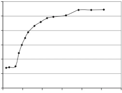
MCPI will have a strong affect on performance. Likewise, MCPI can give a good indication of relative working set sizes of long-running, CPU-bound programs. Such processes’ working set will fill the appropriate level of the memory hierarchy, and the MCPI will reflect the working set size. Figure 1 demonstrates these principles for a simple synthetic workload. An array is iterated through sequentially, and this processes is repeated a large number of times to smooth out anomalies and compulsory misses. Clear plateaus are visible for arrays that fit in the L1 data cache (16 KB), the L3
cache (4 MB), and main memory. In addition, MCPI and performance, represented as the execution time per array element, show the same relative impact at each of the memory hierarchy levels. Note that the execution time per element was omitted from the graph below 32 bytes, since at such a small size the outer loop overhead artificially inflates the execution time per element to above 30 ns.
0 0.5 1 1.5 2 2.5 4 B 1 6 B 6 4 B 2 5 6 B 1 K B 4 K B 1 6 K B 6 4 K B 2 5 6 K B 1 M B 4 M B 1 6 M B 6 4 M B Array Size S ta ll s /i n s tr 5 10 15 20 25 30 T im e ( n s ) Mem stalls/instr ns per element
Figure 1: Memory stall cycles per instruction (left Y-axis) and execution time per array element (nanoseconds, right Y-axis) vs. array size.
Figure 2 shows the MCPI behavior in the L2 cache, whose size at 96 KB is too close to the L1 to be visible in Figure 1. The plateau is not immediately visible because this graph peeks into such a small range; from 16 KB to 50 KB, the plot is rising to the L2 plateau. But from 50 KB to 96KB, the MCPI is roughly constant at 0.5 before increasing to above 0.55 at 96 KB.
MCPI can thus give a good estimate of the relative memory footprint of a process; should the footprint fall outside of the cache, the MCPI will increase dramatically. In order to make this determination, the relative running time of a process must be known. If a process is “long-running” (as demonstrated by this array workload), then its cache behavior falls into place, and MCPI can give an indication of the relative size of the data set among such processes. If a process is “short-running,” there are fewer memory accesses, and even a few L3 cache misses can throw off the MCPI. Thus the MCPI cannot be a good determination of working set size for relatively short-running processes.
0 0.1 0.2 0.3 0.4 0.5 0.6 0 25 50 75 100 125 150 Array Size (KB) S ta ll s /i n s tr
Figure 2: Memory stalls per instruction vs. array size (KB), demonstrating behavior of the L1 data cache (16 KB) and L2 cache (96 KB)
The average running time per scheduling time slice for a process is therefore a necessary metric given this approach. In our tests, even when there was contention in the system among long-running processes (those that displayed expected MCPI behavior based on their data set size), the average time slice was on the order of 10-40 milliseconds. For background processes such as the ssh daemon and sendmail, the average time slice (in user space) remained between .02 to .35 milliseconds. The MCPI for such processes varied wildly, as expected, from 1.3 to in excess of 22. Thus, during scheduling, intelligent decisions using cache affinity for short-running processes cannot be made, given that MCPI does not garner useful information.
Another metric useful for scheduling that can easily be calculated is main memory bandwidth. For a process whose working set fits within one of the processor’s caches, very little main memory bandwidth will be used. The only time an L3 miss is likely to occur is due to a compulsory or conflict miss. However, a process whose working set does not fit in the caches will be accessing main memory far more often due to capacity misses, and will rely on main memory bandwidth to feed the cache hierarchy.
Main memory bandwidth is dependent on the global L3 miss rate, which in turn is independent of the L1 and L2 cache as long as they are less than eight times smaller the size of the L3 cache [3]; every time an L3 access misses, the appropriate cache block must be serviced by the main memory. Thus the general equation to compute memory bandwidth used is:
Bandwidth = memory references / instruction * instructions / cycle * cycles / second * L3 misses / memory reference * bytes / L3 miss [3]
This can be simplified down to:
Bandwidth = L3 misses / cycle * cycles / second * bytes / L3 miss
If one can ignore dirty writes for simplicity’s sake, the number of bytes serviced by an L3 miss is equal to the L3 block size, or 64 bytes in the case of Itanium. Thus only the number of L3 misses and CPU cycles need to be counted in order to estimate memory bandwidth used.
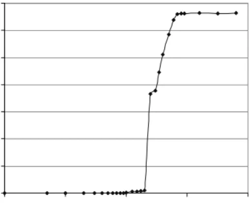
Figure 3 shows the main memory bandwidth used as a function of array size for the previously discussed synthetic workload. The bandwidth used is less than 1 MB/sec until around 4 MB (the L3 cache boundary), at which point a sharp increase brings the bandwidth used to around 130 MB/sec. While this workload is likely artificially low for under 4 MB given that there are very few compulsory and conflict misses, a real workload will likely show a similar dramatic increase in bandwidth consumed as its data set size increases beyond the capacity of the L3 cache. 0 20 40 60 80 100 120 140 0.01 0.1 1 10 100 Array Size (MB) B a n d w id th u s e d ( M B /s e c )
Figure 3: Main memory bandwidth used (MB/sec) vs. array size (MB). Note the sharp increase at 4MB.
While using bandwidth information for CPU scheduling was not attempted due to time constraints, it is foreseeable that such statistics can be useful for an SMP system with a shared bus. With knowledge of the maximum bandwidth that the system bus and main memory can support, a CPU scheduler might
make decisions that prevent the maximum bandwidth from being saturated during a time slice.
4. Methodology
The framework for the CPU scheduler using dynamic performance information utilizes the Linux 2.4.18 kernel. The performance monitoring patch provides the system calls to create performance monitoring contexts, initialize PMC and PMD registers, start and stop performance monitoring, and read the results. The HP pfmon libraries for Itanium [4] provided additional understanding of how software uses Itanium’s performance monitoring model. The Linux Trace Toolkit [6] provided the means to trace performance. The toolkit allows tracing of arbitrary kernel events, and supplies the mechanism for reporting results back to the user-space. Since the toolkit did not provide native support for IA64, it was necessary to port the application to our Itanium system.
The scheduling system was implemented on the HP rx4210 server, with four 800 MHz Itanium processors featuring 16 KB L1 instruction/data caches, a unified 96 KB L2 cache, and an off-chip 4 MB L3 cache. The system has 16 GB of main memory.
5. Approach
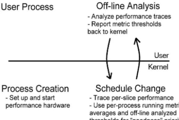
The framework for our system begins at process creation. Upon a fork(), a performance monitoring context is automatically created for all user processes, and the PMC registers are set up to monitor the desired events. The performance monitoring unit (PMU) starts counting the user-space events for the process. In addition, the running averages for the performance metrics (average time slice and MCPI for this case) that are stored in the process’s task_struct are cleared. Figure 4 depicts the performance monitoring and scheduling framework.
Upon every schedule change, the PMD registers of the outgoing process are read and cleared in anticipation of the next scheduling time slice for the process. The running averages of the MCPI and average time slice for the outgoing process are updated, with a weight towards the last time slice. In addition, the raw values of the PMD registers are traced for the user-level off-line analysis.
Figure 4: Framework for the scheduling system using dynamic performance information.
During off-line analysis, the system examines the trace log and coalesces the PMD register traces into per-process totals. The average time slice length and MCPI for each process during the trace period is calculated. This list is then sorted based on the time slice, and divided into two groups. Currently the division is decided by finding the largest ratio between two consecutive time slice values in the list, though a more robust clustering algorithm might be used if more than two groups are desired. The point at which the division occurs can then be used to calculate the threshold for the short-running and long-running processes for the trace period.
The long-running processes are then sorted based on MCPI, and again the division and threshold is obtained. The time slice and MCPI thresholds are then reported back to the kernel.
The frequency of off-line analysis can vary. In principle, tracing and analysis can occur as often as desired. In practice, the tracing and analysis cycle might be performed once every few minutes or hours, with the tracing period lasting 30 – 60 seconds.
The goal of the scheduler modifications is to improve performance for processes with larger memory footprints without sacrificing the performance of the smaller, or shorter-running processes. As of this writing, the former has been accomplished. However, the latter (performance of smaller processes) still needs some fine-tuning. Given that the scheduler has stall cycle and threshold information, it can determined whether a given process has a larger or smaller memory footprint. The cache context is much more valuable to the larger processes, and therefore critical to their performance. We believe that in order to improve performance of larger processes, the following two conditions should hold:
1. The larger processes should be evenly distributed across available processors. That is, on a 4-processor system, 4 larger processes should each be running on a separate processor, no matter how many smaller processes are in competition with them.
2. The larger processes should be consistently running on the same processor. This allows for optimal cache context reuse.
Violating either of these conditions destroys the cache context of the process: the context will be destroyed by the competing larger process in the first case, and lost because of the processor move in the second case.
The implementation of the two goals specified above turns out to be a challenge. The major difficulty arises when dealing with the single process queue that is part of the 2.4 scheduler. Ensuring condition 2 is far from straightforward, and becomes even more difficult when taken together with the first condition.
We modified the goodness() function to give a much better estimate of cache affinity. Namely, the static parameter that estimates the cache affinity is now scaled by the actual value of memory stalls per cycle. This weight is only added to the process' priority in the case its previous CPU is the same as the one it is being considered for. This modification attempts to take care of the second condition.
The first condition implies two larger processes should be discouraged from running on the same
processor. We modified the
preemption_goodness() function to scale down the value it returns in case both the previous and the new process are above the threshold calculated in the off-line analysis phase. Another point where modification was needed is in the case where a processor becomes idle and is looking for a new process to run. The code was likewise modified to scale down the goodness() value if both the previous and the new process are above the threshold. The current implementation is not fully fine-tuned. The response time of smaller and shorter-running processes decreased somewhat in our experiments. However, it provides a good first approximation of how to modify the scheduler to take advantage of dynamic performance statistics. Our work is also readily applicable to Linux 2.5 scheduler [8], which has multiple queues, one per processor. The multiqueue feature allows for much easier implementation of the two conditions specified above. Particularly, ensuring that a process stays on a processor is virtually automatic.
While this system uses MCPI to aid in scheduling and off-line analysis to determine thresholds, the basic framework remains the same regardless of the use. It should be relatively simple to count different events, use the off-line analysis for different purposes, and change the use of dynamic performance information in scheduling.
6. Results
First, results using the default Linux 2.4 scheduler will be analyzed, followed by a discussion of the benchmarks using scheduling with dynamic performance information.
6.1 Performance with the Default Linux Scheduler
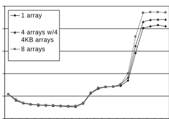
In order to show the effects of cache affinity in CPU scheduling, contention must be introduced into the system using the synthetic array workload. Figures 5 and 6 show the same workload as figure 1, with the former graphing memory stall cycles per instruction vs. array size and the latter displaying execution time per element vs. array size. The baseline performance of iterating through one array is included for comparison.
0 0.5 1 1.5 2 2.5 4 B 1 6 B 6 4 B 2 5 6 B 1 K B 4 K B 1 6 K B 6 4 K B 2 5 6 K B 1 M B 4 M B 1 6 M B 6 4 M B Array Size M e m s ta ll s / i n s tr 1 array 4 arrays w/4 4KB arrays 8 arrays
Figure 5: Memory stall cycles per instruction vs. array size for three workloads: iterating through one array, concurrently iterating through four arrays of the specified size along with four 4 KB arrays, and concurrently iterating through eight arrays of the specified size.
The first line to note is for the workload that iterates through eight arrays simultaneously. In such a workload, the operating system multiplexes the four
CPUs evenly among the eight arrays, and a process never stays on the CPU where its cache contents are located. At large data set sizes, the arrays effectively clobber the cache contents of whatever array previously ran on the processor, and the memory stall cycles per instruction and execution time per element show a hit in performance. With this many processes in the system, the contention allows the constant cache affinity value added to priority to keep processes on the same processor. But with eight large arrays in the system, there exists the possibility that cache contents can be kicked out by another array. Thus, given that there are four processors, arrays of sizes 2 MB and larger perform worse than the baseline. At 16 MB, the memory stall cycles per instruction are 2.19 vs. 1.86 for the baseline; likewise, the execution time per element is 28.7 ns vs. 25.5 ns for the baseline. It should be noted that the execution time per element uses per-process running time instead of wall clock time, since obviously with eight CPU intensive processes running on four processors, the wall clock execution time will be at least twice as long.
5 10 15 20 25 30 3 2 B 1 2 8 B 5 1 2 B 2 K B 8 K B 3 2 K B 1 2 8 K B 5 1 2 K B 2 M B 8 M B 3 2 M B Array Size n s p e r e le m e n t 1 array 4 arrays w/4 4KB arrays 8 arrays
Figure 6: Execution time per element (nanoseconds) vs. array size for three workloads: iterating through one array, concurrently iterating through four arrays of the specified size along with four 4 KB arrays, and concurrently iterating through eight arrays of the specified size.
The second workload tested iterates through four arrays of the size specified by the x-axis along with four 4 KB arrays. This is a synthetic workload that can demonstrate possible improvement should the scheduler be aware of the working set sizes of the processes. In such a workload, it is desirable for the larger arrays to stay on their own processor, while the
4 KB arrays are multiplexed among the available processors. Running a 4 KB array along with one of the larger arrays (1+ MB) will not destroy the L2 and L3 cache contents of the larger array. Should the larger array remain on the same processor when it preempts one of the 4 KB arrays, it will not have to deal with compulsory misses in the L2 and L3 caches. While the default Linux scheduler tends to keep processes on the same CPU, it does not differentiate between the working set sizes of the processes. Thus two large arrays can stay on the same CPU and continually kick out each other’s cache contents. At 8 MB, the memory stall cycles per instruction are 2.02 vs. 1.86 for the baseline; the execution time per element is now 27 ns vs. 25.5 ns for the baseline.
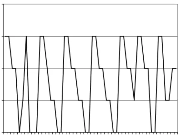
0 1 2 3 4 1 4 7 10 13 16 19 22 25 28 31 34 37 40 43 46 49 Slice number C P U
Figure 7: CPU on which an array runs vs. time slice number.
Another workload that the default Linux scheduler displays inadequate behavior is when there is not enough contention in the system for the constant cache affinity value to affect priority. Figure 7 demonstrates the lack of processor affinity when there are three 3 MB arrays along with two 4 KB arrays. There exists the possibility for cache affinity since the three large arrays can distribute themselves on separate processors. But when a processor becomes idle, there is typically only one process in the ready queue, so it will get scheduled on the CPU regardless of where it previously ran. The time slice in this case is roughly constant, so the x-axis represents time. Each time an array is scheduled, it runs on a different processor, thus losing the benefit of cache affinity.
6.2 Performance with the Scheduler using Dynamic Performance Information
In order to test the effectiveness of the dynamic performance scheduler, a workload with enough contention for scheduling to be effective is necessary. The test workload iterates through four 3 MB arrays and six 4 KB arrays simultaneously. This gives the possibility for the four larger arrays to distribute themselves and use the L2 and L3 caches effectively, while the six smaller arrays create enough contention in the system for scheduling to matter while maintaining the L2 and L3 contents of the larger arrays. With larger array sizes of 3 MB, the arrays will effectively clobber each others’ cache contents should they not remain on separate CPUs. Table 1 summarizes the results for the default Linux 2.4 scheduler, the dynamic performance scheduler before the time slice and MCPI thresholds have been set, and the dynamic performance scheduler after the thresholds have been set.
Table 1: MCPI, execution time per array element (nanoseconds), and wall clock execution time (seconds) for simultaneous iteration through four 3 MB arrays and six 4 KB arrays. This test is performed on the default Linux 2.4 kernel, the dynamic performance scheduler before setting the thresholds, and the dynamic performance scheduler after setting the thresholds.
The default Linux kernel uses its constant cache affinity parameter to help processes remain on the same CPU for longer periods of time, but it treats the two differently-sized arrays the same. The dynamic performance scheduling system without the thresholds set breaks this behavior; since all processes jump around CPUs with each scheduling time slice, cache affinity is worsened and the MCPI and execution time per element suffers. The dynamic performance scheduler with the thresholds set improves cache affinity over the default Linux scheduler; MCPI shows a 9.3% increase and execution time per element shows a 12.8% increase. Wall clock time, which is 4.5% worse, likely suffers due to the overhead added to the scheduler. There
MCPI
exec
time/element wall clock time
default Linux kernel 0.8402 13.32 ns 23.70 sec dynSched w/o thresh 0.9515 16.13 ns 29.53 sec dynSched w/ thresh 0.7687 11.8 ns 24.76 sec
still is much optimization that can be done, so this figure could likely be reduced.
6.3 Overhead
Any OS modification must be evaluated in light of its overhead. After all, OS functions are just overhead to the user. Scheduling is a task particularly sensitive to any extra baggage, since it runs quite often. The overhead of our framework is split between the scheduler, tracing events and the offline analysis.
The scheduler overhead consists largely of the extra bookkeeping done on every context switch. The updates to the running totals for average time slice and memory stalls take up much of the overhead. The extra calculations needed for determing the goodness() are a smaller part. Some of the bookkeeping could be moved a less time-critical section of the kernel. Perhaps an update every few seconds (milliseconds) would be sufficient.
Linux Trace Toolkit imposes an overhead of less than 2.5% on overall performance [13]. Our changes do not add significant overhead. Further, the events are not being traced continuously. Rather, a sample trace is taken every few minutes or every few hours, depending on the workload. Similarly, the offline analysis is invoked rarely, and only in order to analyze the trace. Our current implementation takes only about 0.65 seconds of CPU time.
7. Related Work
The inspiration for our system comes from a variety of previous work on in-situ simulation and self-modifying systems. However, while our system aims to improve SMP scheduling performance with analysis at a fine-granularity, much of the previous work is targeted towards batch scheduling on large-scale parallel systems using coarse-granularity analysis.
Seltzer et al. propose monitoring and self-adapting operating systems [10]. Using VINO’s grafting architecture, traces and logs are statically gathered and analyzed to determine what the system is doing. Off-line analysis is performed once a day and compared to previous logs, and on-line analysis is responsible for instantaneous monitoring of changes in resource utilization. The use of hardware performance counters is proposed for analyzing CPU-bound processes; if it is determined that branch prediction or cache accuracy is too low, recompilation of poorly-performing kernel functions
can be requested. The recompiled kernel segments can then be grafted into the kernel.
Nguyen et al.’s system uses in-situ simulation to dynamically determine the optimal number of processors to allocate to a process on a large-scale shared memory parallel system [8]. Since parallel applications can see speedups that are data and time-dependent, system efficiency is increased when CPU allocation is decided on a need basis. Their runtime system dynamically measures job efficiencies at different locations, uses the results to measure speedup, and adjusts processor allocation to maximize speedup.
Streit argues that the performance of job scheduling policies depends on scheduled jobs [11]. In his system, a self-tuning scheduler constructs virtual schedules for each policy (Come First-Serve, Shortest Job First, and Longest Job First) at every scheduling decision. If the simulation finds that an alternate policy can produce better performance with the current workload, the scheduler immediately switches to that policy. His work is aimed at batch processing on large-scale systems, such as the IBM SP2 and ASCII Blue.
Feitelson et al. [2] propose conducting simulations on log files during the operating system’s idle loop that can optimize scheduling parameters. They use genetic algorithms to find optimized values, and they improve batch scheduling on an Intel iPSC/860 hypercube supercomputer.
8. Conclusion
We have proposed a framework by which dynamic performance can be traced and analyzed in order to make better scheduling decisions. Our system levies the hardware performance counters in modern microprocessors to gain better information about what processes are doing at run-time.
The first goal for the use of this framework was to improve cache affinity in an SMP system. The default Linux scheduler does succeed in some situations in keeping processes on the same processor in order to maintain cache affinity, but it does not take cache usage into account. Our use of the dynamic performance information improves cache performance. While the current implementation still requires fine-tuning, it provides an example of how the framework can be used.
While using more performance metrics can lead to better scheduling decisions, we are faced with the problem that Itanium does not contain enough performance counting registers to successfully
monitor more than a few metrics simultaneously. Perhaps the expanded use of performance hardware will lead to more robust implementations in the future.
This framework opens up possibilities for other dynamic scheduling applications. The scheduler can manage memory bandwidth, another resource that critical for performance in an SMP system. Seltzer proposes [10] that branch predictor and TLB performance can also be used. A fair-share scheduler can also use this framework to allow sharing of resources other than CPU time. Thus, the field of dynamic performance tuning still has a multitude of unexplored avenues.
References
[1] D. P. Bovet and M. Cesati. “Understanding the Linux Kernel.” O’Reilly: Sebastopol, CA, 2001. [2] D.G. Feitelson and M. Naaman. Self-Tuning
Systems. In IEEE Software 16(2), pages 52--60, April/May 1999.
[3] J.L. Hennessy, D.A. Patterson. Computer Architecture: A Quantitative Approach, 3rd Ed. Morgan Kaufmann, 2001.
[4] The HP pfmon library package for the IA64 / Itanium Performance Monitoring Unit. ftp://ftp.hpl.hp.com/pub/linux-ia64/pfmon-1.1.tar.gz
[5] IA-64 Processor Reference: Intel® Itanium™ Processor Reference Manual for Software Development. Revision 2.0, December 2001. http://developer.intel.com/design/itanium/downl oads/245320.htm
[6] The Linux Trace Toolkit.
http://www.opersys.com/LTT/
[7] J. McCormick and A. Knies. A Brief Analysis of SPEC CPU2000 Benchmarks on the Intel® Itanium™ 2 Processor. Hot Chips 2002.
[8] I. Molnar. "Ultra-scalable O(1) SMP and UP scheduler".
http://www.uwsg.iu.edu/hypermail/linux/kernel/ 0201.0/0810.html
[9] T. D. Nguyen, R. Vaswani, J. Zahorjan. Maximizing Speedup through Self-Tuning of
Processor Allocation. In Proceedings of the 10th International Parallel Processing Symposium, pages 463--468, Waikiki, HI, Apr. 1996.
[10] M.I. Seltzer and C. Small. Self-monitoring and Self-adapting Operating Systems. 6th Workshop on Hot Topics in Operating Systems (HotOS-VI), Rio Rico, AZ, March 1997.
[11] A. Streit. A Self-Tuning Job Scheduler Family with Dynamic Switching Policy. In Proceedings of the 8th Workshop on Job Scheduling Strategies for Parallel Processing (JSSPP) at the 11th International Symposium on High Performance Distributed Computing (HPDC-11). [12] C. A. Waldspurger and W. E. Weihl. Lottery scheduling: Flexible proportional-share resource management. In Proceedings of the First Symposium on Operating System Design and Implementation (November 1994), pp. 1-11. [13] K. Yaghmour and M. Dagenais. Measuring and
Characterizing System Behavior Using Kernel-Level Event Logging. Proceeding of the 2000 Usenix Annual Technical Conference, 2000.