Communication-Efficient Federated Learning for
Wireless Edge Intelligence in IoT
Jed Mills, Jia Hu*, Geyong Min*
Abstract—The rapidly expanding number of IoT devices is generating huge quantities of data, but public concern over data privacy means users are apprehensive to send data to a central server for Machine Learning (ML) purposes. The easily-changed behaviours of edge infrastructure that Software Defined Networking provides makes it possible to collate IoT data at edge servers and gateways, where Federated Learning (FL) can be performed: building a central model without uploading data to the server. FedAvg is a FL algorithm which has been the subject of much study, however it suffers from a large number of rounds to convergence with non-Independent, Identically Distributed (non-IID) client datasets and high communication costs per round. We propose adapting FedAvg to use a distributed form of Adam optimisation, greatly reducing the number of rounds to convergence, along with novel compression techniques, to produce Communication-Efficient FedAvg (CE-FedAvg). We per-form extensive experiments with the MNIST/CIFAR-10 datasets, IID/non-IID client data, varying numbers of clients, client par-ticipation rates, and compression rates. These show CE-FedAvg can converge to a target accuracy in up to6×less rounds than similarly compressed FedAvg, while uploading up to3×less data, and is more robust to aggressive compression. Experiments on an edge-computing-like testbed using Raspberry Pi clients also show CE-FedAvg is able to reach a target accuracy in up to1.7×
less real time than FedAvg.
Index Terms—Federated Learning, Internet of Things, Dis-tributed Computing, Edge Computing, Compression.
I. INTRODUCTION
T
HERE are over 8 billion Internet of Things (IoT) devices worldwide, as of 2019 [1]. These are typically low-powered, embedded devices used for data collection. The expansion of the number of IoT devices has therefore led to an explosion in the quantity of data available for organisations to use for Machine Learning (ML) purposes. These organisations can use this data for insights, consumer products, and scientific research. However, there is growing public concern over the distribution of private data. Many IoT devices, such as security cameras, fitness and health trackers and smartphones gather sensitive data that users would not wish to share with a central server.The combination of increasing IoT devices and data, along with user privacy concerns presents a series of opportunities and challenges for ML. There is the potential to use the large number of IoT devices to perform distributed ML, rather
J. Mills, J. Hu and G. Min are with the College of Engineering, Maths and Physical Science, University of Exeter, United Kingdom. E-mail: {jm729, j.hu, g.min}@exeter.ac.uk.
* Corresponding authors.
Copyright (c) 20xx IEEE. Personal use of this material is permitted. However, permission to use this material for any other purposes must be obtained from the IEEE by sending a request to [email protected].
than in a central server, distributing expensive training and inference while keeping private data on user devices. However, distributed ML schemes are typically designed for the data-centre, assuming high performance computing and networking hardware, contrasting the highly heterogeneous computing and communication capabilities of low-powered IoT devices. Also, IoT devices collect data from different users, so the distribu-tion over devices can be highly non-Independent, Identically Distributed (non-IID), making it difficult to create ML models with good performance.
Software Defined Networking (SDN) has the potential to help alleviate some of the distributed ML problems. Edge network architecture typically involves IoT devices connected to IoT gateways. Gateways and similar devices often possess much more computing and storage capacity than IoT devices and are located at the network edge, closer to user devices, meaning data does not need to be centrally collected. SDN could be used to easily alter the behaviour of IoT gateways: collecting data from a group of local IoT devices and perform-ing distributed ML, or deliverperform-ing these data securely to nearby edge servers.
To address the issue of distributed ML, the concept of Federated Learning (FL) [2] – collaboratively training a model across devices without sharing their data – was introduced. McMahan et al. [3] proposed an implementation of FL with their FedAvg algorithm, designed for user devices such as smartphones. In FedAvg, clients independently train Deep Neural Networks (DNNs) on their local data and periodically average them. FedAvg has been shown to work in real-world settings by Google with their GBoard [4] next-word-prediction and emjoi-prediction [5] software. FedAvg can be used in the IoT/SDN framework described above to provide distributed ML at the network edge.
Modern DNNs contain a huge number of weights, in the order of tens to hundreds of millions. As FedAvg requires uploading and downloading these models between the clients and the central server, several works have been published on reducing the amount of communication performed by FedAvg to reduce bottlenecks and help ease network use.
A standard method of training DNNs is minibatch-Stochastic Gradient Descent (mb-SGD): model weights are updated with their gradients multiplied by a fixed learning rate. Most works on FL use mb-SGD for their DNNs, however, there are more sophisticated optimisation techniques based on mb-SGD, such as AdaGrad [6] and RMSProp [7]. Adam [8] is one popular technique that features both per-parameter learning rates and momentum. It has been shown to be a very efficient optimizer for many tasks, and has the potential to
improve the convergence rate of FedAvg.
FedAvg therefore has the following problems when con-sidered with the IoT edge-computing scenario. First is the high communication cost per round due to large models being sent between the clients and the server, and the second is the high number of rounds to convergence, especially in non-IID settings. This paper proposes Communication-Efficient FedAvg (CE-FedAvg), which reduces the number of rounds to convergence, and the total data uploaded per round over Fe-dAvg. We therefore make the following contributions:
• Proposal of the CE-FedAvg algorithm, which is com-posed of two parts: distributed Adam optimisation and compression of uploaded models. CE-FedAvg reduces the number of communication rounds taken to reach a target accuracy, and the total data uploaded per round compared to uncompressed FedAvg.
• We develop two novel schemes for the quantization of
communicated weights and moment values of Adam (Uniform and Exponential Quantization). These two schemes are used alongside sparsification and Golomb encoding for the compression in CE-FedAvg.
• Extensive simulated experiments of CE-FedAvg using the MNIST and CIFAR-10 datasets, three DNN architectures, and varying numbers of clients and client participation rates. These show CE-FedAvg is able to reach a target accuracy in far fewer rounds than FedAvg in non-IID scenarios, and that it is more robust to aggressive com-munication reduction.
• Further experimentation on an edge-computing-like testbed using Raspberry Pi clients show CE-FedAvg reduces the real time to convergence over FedAvg. The remainder of this article is structured as follows: we outline related work in the fields of FL and ML for the IoT; we then describe our proposed algorithm, CE-FedAvg, in detail; after that we outline the simulation and testbed experiments we ran comparing CE-FEdAvg to FedAvg; and we finally give our conclusions of this work in the last section.
II. RELATEDWORK
A. Federated Learning
McMahan et al. [3] proposed the original FedAvg algorithm to train an aggregate model without uploading client data to a server. FedAvg drastically reduces total communicated data compared to datacentre-style distributed SGD (where each worker performs a single step of SGD before aggrega-tion).
FL considers clients with non-IID data distributions, which is an obstacle to training a good central model. Zhao et al. [9] proposed sharing a small amount of data between non-IID clients to reduce the difference between clients distributions, increasing the maximum accuracy their FedAvg models were able to attain.
Devices participating in FL are assumed to have highly het-erogeneous computing and networking resources. Wang et al. [10] addressed this with a control algorithm that dynamically changes the number of local SGD updates that clients perform before uploading their models, based on a trade-off between
the computing power and networking bandwidth available to the client.
Several papers have been written on the task of reducing the amount of data communicated during FedAvg. Koneˇcn´y et al. [11] introduced the concepts ofstructured andsketched model updates, and were able to significantly reduce the quantity of uploaded data during training. Similarly, Sattler et al. [12] demonstrated theirSparse Binary Compressionsystem against uncompressed FedAvg, and were able to achieve better accuracy while communicating much less data. Lin et al. proposed Deep Gradient Compression [13], a system applicable to FedAvg, where gradient updates are accumulated at clients until their magnitude is greater than a threshold. Sattler et al. [14] proposed Sparse Ternary Compression to compress weight updates during FedAvg, including using Golomb Encoding [15] to compress the indexes of weights in sparse matrices produced by sparsification.
As well as compression of weights, other techniques to reduce communication during FedAvg have been proposed. Chen et al. [16] aggregated shallow layers more frequently than deep layers (they assert that shallow layers learn general features and deep layers learn more specific features). Their scheme was able to converge to a target accuracy with up to 7×less communication than FedAvg. Liu et al. [17], proposed having clients aggregate with intermediate servers which then aggregate with a main server with two given frequencies. Their experiments showed that increasing aggregation frequency causes the global model to converge faster (as would be expected), and that the global aggregation frequency has the biggest impact on convergence rate.
Leroy et al. [18] proposed adapting the Adam optimizer to the FedAvg algorithm. In their system, clients perform SGD using all their local data, and send their weight updates to the server. The server holds 1st and 2nd moment values for each
weight, which it uses to compute the central model weight updates using the Adam update rule. However, the way we use Adam is different in our work from [18]: our method uses Adam optimisation at clients, and the Adam values are also aggregated at the server, as opposed to using Adam solely at the server. We also propose compression schemes for our version, which Leroy et al. do not.
B. Internet of Things and Machine Learning
Some works have been published combining Deep Learning and the IoT. One seminal work by Liu et al. [19] created a system for identifying foods. In it, image preprocessing and segmentation was performed on edge devices, and classifi-cation was done on a central server, reducing the latency at inference time. Li et al. [20] put forward a similar idea where a ML model was trained in the cloud, then initial layers of the model were distributed to edge servers. At inference time, the edge servers compute the first layers before sending the result of these to the cloud for the final inference, resulting in less data sent to the cloud over sending the raw input.
For training near the network edge, Kyu et al. [21] created Fog Privacy-Preserving Deep Learning (FPPDL), which com-bines privacy-preserving techniques with intermediate-layer
aggregation of IoT data at ‘Fog’ nodes before aggregation with a central server.
ML has been applied to a large variety of edge-like devices. Reina et al. [22] treated Unmanned Aerial Vehicles (UAVs) as edge devices, and solved the Multi-Objective Optimization Problem for their area coverage using a Multi-Subpopulation Genetic Algorithm.
Pathinarupothi et al. [23] developed a unique IoT-based system to provide health alerts to doctors for patients. Patients were fitted with multiple physiological sensors, which could be connected to the internet using the patient’s smartphone as a gateway. The gateways had software to determine if doctors need be alerted of patients. This system shows the ability for smartphones to be used as intelligent, programmable gateways for nearby IoT devices, which could be applicable to the scheme proposed in this work.
Other authors have investigated the resource consumption of DNNs on IoT and edge devices. Chandakkar et al. [24] developed a system for re-training and pruning networks at the edge as nodes receive data over time. Similarly, DeepIoT [25] was created to reduce the size of DNNs for inference by using a second network to determine the best weights to drop from the original network. Guo et al. [26] proposed a novel approach that involved training a DNN and using an automata to gradually prune the network weights over time. They were able to slightly improve the MNIST performance of dense networks with this method while pruning >40% of weights.
Most current work exploring ML and the IoT focuses on centralised training, and using IoT/edge computing for inference, or on decreasing the size of DNNs for these devices. This work, however, investigates decentralised training using full DNNs.
III. CE-FEDAVG
The FedAvg algorithm has a single master model that is an aggregate of client models. For each round of communication, the server selects a subset of clients and pushes the master model to these clients. Each client then performs a predeter-mined number of rounds of gradient descent using the client’s local data, pushes their model weight deltas to the server, and the server then averages these updates to become the new master model.
FedAvg features a fixed learning rate across devices as per normal mb-SGD. As shown below, this can result in a very large number of rounds required to converge to a given accuracy. mb-SGD can result in low convergence rates in later rounds of training because some weights need finer ‘tuning’ than others. Adam optimization is a popular alternative to standard mb-SGD. It stores two values for each model weight:
m (the 1st moment) and v (the 2nd moment), which are
used along with gradients computed by backpropagation and global decaying learning rates to update model weights for each minibatch. Adam reduces both the problems of weights requiring different degrees of tuning (having adaptive rates for each weight), and local minima (via momentum).
Alongside this, in FedAvg, the entire DNN model is sent from clients to server each round. Modern DNNs have a
Fig. 1. One communication round of CE-FedAvg: 1. Clients download the global model weights, 1st and 2nd moments (ω, m, v); 2. Clients perform
training on their IoT-derived datasets; 3. Clients compress their models; 4. Clients upload their compressed parameters and indexes (ω0, m0, v0, i); 5. The
server decompresses the model weights and moments; 6. The server aggregates all client models before starting a new round of training.
huge number of weights, and the upload bandwidth of edge clients is typically far lower than the download bandwidth. Therefore, uploading models to the server is a significant potential bottleneck of the system. Previous works have shown that these uploaded weight tensors can be compressed without significantly harming the performance of the model [11] [12] [13] [14]. However, these schemes typically increase the number of rounds FedAvg takes to converge, albeit with lower total data uploaded by clients.
To address the above problems, we propose CE-FedAvg: a scheme that both reduces the number of rounds taken to converge to a given accuracy and decreases the total data uploaded during training over FedAvg. Algorithm 1 shows the details of CE-FedAvg. The UniQ, UniDQ, ExpQ and ExpDQ functions are shown in Algorithms 2 and 3.
In CE-FedAvg, the server first initialises the global model with random weights and 0 values for the 1st and 2nd Adam moments (line 3). Each communication round, the server selects a subset of clients (line 5) and sends the weights and moments to them. In our algorithm, clients are selected at random, but in reality clients would be selected based on their power/communication properties at the time as in [4]. These clients then perform their local Adam SGD (lines 7-8), and upload their data to the server. The server dequantizes and reconstructs the sparse updates from the clients (lines 10-17), averages the updates (lines 20-22) and starts the next round. Each client updates by replacing their current model with the downloaded global weights and moments (line 27), performing E epochs of Adam SGD (lines 28-34), sparsifying and then quantizing the model deltas and sparse indexes (lines 36-40)
and uploading the model to the server. Barring compression, CE-FedAvg would communicate3×the data as FedAvg (the shapes ofmandvare the same asω). However, as shown later,
ω, m and v can be aggressively compressed in CE-FedAvg while still taking less rounds to converge than FedAvg. Algorithm 1 CE-FedAvg
1: Server Executes:
2: // Global weights, 1st and 2nd moments
3: initialise ω;m←0;v←0
4: whiletermination condition not metdo
5: S← random set ofmax(C·K,1) clients 6: for each k∈S in paralleldo
7: (ωq,mq,vq, g, b∗, lzmin, lzmax, gzmin, 8: gzmax, bm, bv)←ClientUpdatek(ω,m,v)
9: // Decompress deltas and indexes
10: ∆ωk←0
11: ∆mk ←0
12: ∆vk ←0
13: idxs←GDecode(g, b∗)
14: ∆ωk,idxs←UniDQ(ωq, lzmin,
15: lzmax, gzmin, gzmax)
16: ∆mk,idxs←ExpDQ(mk, bm) 17: ∆vk,idxs←ExpDQ(vk, bv) 18: end for
19: // Update global weights
20: ω←ω+PKk=1nk n∆ωk 21: m←m+PK k=1 nk n ∆mk 22: v←v+PK k=1 nk n ∆vk 23: end while 24:
25: function CLIENTUPDATEk(ω,m,v) 26: // Client weights, 1stand 2nd moments
27: ωk←ω;mk←m;vk ←v 28: forepoch←1 :E do
29: batches←(dataPk in batches of size B) 30: for eachb∈batchesdo
31: // Perform Adam gradient descent
32: ωk,mk,vk ←AdamSGD(ωk,mk,vk)
33: end for
34: end for
35: // Compress ωk,mk,vk deltas and indexes 36: ωs, idxs←Sparsify(ωk−ω)
37: g, b∗←GEncode(idxs)
38: ωq, lzmin, lzmax, gzmin, gzmax←UniQ(ωs) 39: mq, bm←ExpQ(mk−m)
40: vq, bv←ExpQ(vk−v)
41: Return (ωq,mq,vq, g, b∗, lzmin, lzmax, 42: gzmin, gzmax, bm, bv) to server 43: end function
CE-FedAvg provides other practical benefits over FedAvg. Due to the adaptive learning rates inherited from Adam, CE-FedAdam works well with the default Adam parameters. FedAvg, on the other hand, requires finding learning rates for each specific dataset and scenario [3]. Not only is this time-consuming and costly, but in the FL setting, the server does not have access to client datasets, so it is unclear how this would
be done in reality. Also, as CE-FedAvg reduces the number of rounds of communication to reach a target accuracy, the total amount of computation required of clients is also reduced: the extra cost of performing one round of CE-FedAvg over FedAvg is outweighed by reduced rounds of learning. We are not aware of any work on FL that reduces the amount of computation at clients in this way.
IV. COMPRESSIONSTRATEGIES
Previous work compressing the models uploaded by clients typically rely on sparsification of weights and/or quantization of weights from typical 32-bit floats.
Algorithm 2 Uniform Quantization (UniQ) and Dequantiza-tion (UniDQ) 1: function UNIQ(a) 2: lzmin ←min(a−) 3: lzmax←max(a−) 4: gzmin ←min(a+) 5: gzmax←max(a+)
6: q←0|a|// initialise q, type 8-bit int
7: qa<0← blz 127
max−lzmin(aa<0−lzmin)c
8: qa>0←128 +bgz 127
max−gzmin(aa>0−gzmin)c
9: returnq, lzmin, lzmax, gzmin, gzmax 10: end function
11:
12: function UNIDQ(q, lzmin, lzmax, gzmin, gzmax) 13: d←0|q|// initialise d, type 32-bit float
14: dq<128←(lzmax127−lzminqq<128) +lzmin
15: dq≥128←(gzmax127−gzmin(qq≥128−128)) +gzmin 16: returnd
17: end function
Our proposed technique comprises of sparsification fol-lowed by quantization. To sparsify gradients, for each tensor, the top (s−1)% of deltas with the largest absolute value are chosen, and they are extracted along with their (flattened) indexes. In CE-FedAvg, the correspondingmandvdeltas are also sent along with the weight deltas, using the same indexes. We found that if non-correspondingm andv values are sent (i.e. the m andv tensors are sparsified independently, in the same manner as the weight tensors) this quickly produces exploding gradients at the clients, likely due to stale m
and v values producing problems in the Adam optimization algorithm.
After sparsification, the weight deltas, m andv are quan-tized from 32-bit floats to 8-bit unsigned ints. The weight deltas contain positive and negative values with the greatest (s−1)%of magnitudes, and are quantized as per theUniform Quantizationscheme shown in Algorithm 2. To quantize using Uniform Quantization, the values with the greatest positive and greatest negative, and lowest positive and lowest negative are chosen (lines 2-5). These are used to map all values lower than zero to the integers 0-127 (line 7) and values greater than zero to 128-255 (line 9). To dequantize, the reverse functions are applied (lines 14-15) to return a vector of floats.
Analysis of m andv values produced by Adam show that there is a large range in the scale of these values: the authors
experiencing values with exponents ranging from 10−1 to to
10−35. Attempts to quantize m andv deltas show that they
are very sensitive to errors in their exponent, and quantizing them using Uniform Quantization or schemes from other works results in exploding gradients within a few rounds. Therefore, we propose a different method of quantization, dubbed Exponential Quantization, for these deltas.
Algorithm 3 Exponential Quantization (ExpQ) and Dequan-tization (ExpDQ)
1: function EXPQ(a) 2: b←min(abs(a))1271
3: q←0|a| // initialiseq, type 8-bit int
4: p← blog1(b)log(abs(a))c 5: qa<0←abs(pa<0)
6: qa>0←128 +abs(pa>0)
7: return q, b 8: end function
9:
10: function EXPDQ(q, b)
11: d←0|q| // initialised, type 32-bit float
12: d0<q<128← −b−q0<q<128
13: dq≥128←b128−qq≥128
14: return d
15: end function
In Exponential Quantization, negative values are again mapped to the range 0-127, and positive to 128-255. Algorithm 3 shows the procedure. To quantize a tensor, the smallest absolute value, δ, is found, and b = δ−1/127 is computed
(line 2). This provides thebasefor quantization: the minimum base with exponent of 127 able to represent the value with the smallest magnitude in the tensor. Using the minimum possible base provides the highest resolution for the quantized values. The logarithm with base b for all values in the tensor is then found and rounded to the nearest integer (line 4), with 128 added to positive values to map them to 128-255 (line 6). To dequantize,bis simply raised to the power ofqfor each value, times by−1 forq<128 (lines 12-13).
The last item to be compressed are the indexes of the values in the sparse arrays sent from clients to server. For these values, we use the lossless Golomb Encoding [15] technique as used by Sattler et al. [14] in their Sparse Ternary Compression scheme.
Using these techniques, compressed FedAvg therefore up-loads for each weight tensor: the weight deltas (8-bit integers); the four min/max values from Uniform Quantization (4×32 bits); their indexes (Golomb encoded); and b∗ (a 32-bit float used for Golomb encoding). CE-Fedvgm must communicate all of these, plus the mandvdeltas (both 8-bit integers) and the base, b for both of these from Exponential Quantization (32-bit floats). The total number of uploaded bits after com-pression, per client per round, is therefore:
FedAvg:bitsup= 160|W|+ (1−s)(8 +gs) X ω∈Ω |ω| (1) CE-FedAvg: bitsup= 224|W|+(1−s)(24+gs) X ω∈Ω |ω| (2) where s is the sparsity, Ω is the set of weight tensors comprising the network, and gs is the expected number of
bits needed to Golomb encode one index value for a given sparsity.
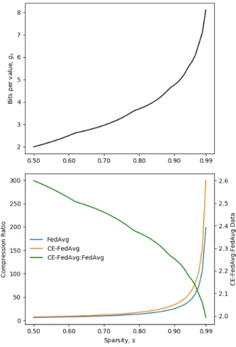
Fig. 2. Top:expected number of bits per value,gs, using Golomb Encoding versus sparsity.Bottom:compression ratio of CE-FedAvg and FedAvg, and CE-FedAvg:FedAvg uploaded data ratio versus sparsity.
The implementation of Golomb Encoding (GE) [15] is the same as used in [14]. The expected number of bits per value for a given sparsity,gs, is given as:
gs=b∗+ 1 1−s2b∗ (3) b∗= 1 +blog2(φ−1 s )c (4) whereφ= √ 5+1
2 ≈1.62is the golden ratio. The value ofb
∗
is sent from client to server to convert the GE bit string back to integer values.
Plotting gs (Figure 2, top), the second terms of the above
equations, and the nominal (without |W| terms) ratio of CE-FedAvg to CE-FedAvg uploaded data with different s (Figure 2, bottom) shows that CE-Fedvg compresses more than FedAvg using this scheme. This means the total amount of data uploaded by a CE-FedAvg client in a single round is between 2.6−2×that of FedAvg for0.5≤s <1.0, as opposed to3×
if there was no compression. However, despite communicating 2−2.6×more data than FedAvg per client per round, due to the reduction in rounds achieved by CE-FedAvg, clients still upload less total data than FedAvg in many cases.
V. EXPERIMENTS
A. Simulation Setup
A series of experiments were conducted to evaluate CE-FedAvg against CE-FedAvg. The experiments were image classification tasks using the MNIST [27] and CIFAR10 [28] datasets. Models were implemented using Tensorflow [29].
MNIST: 28×28 greyscale images of handwritten digits in 10 classes. Two models were trained on this dataset. The first (MNIST-2NN) had two fully connected layers of 200 neurons with ReLU activation, and a softmax output layer. The second (MNIST-CNN) was a convolutional network consisting of: two 5 ×5 convolutional layers with 32 and 64 output neurons, respectively, each followed by 2×2 max pooling and ReLU activation; a fully connected layer with 512 neurons and ReLU activation; and a softmax output layer. CIFAR10: 32×32 colour images of objects in 10 classes. One network (CIFAR-CNN) was trained on this dataset with: two3×3convolutional layers with 32 output neurons, L2 regularization and each followed by batch normalization; a dropout layer with d= 0.2, two 3×3 convolutional layers with 64 output neurons, L2 regularization, and batch normalization; a second dropout layer with
d= 0.3; two final 3×3 convolutional layers with L2 regularization and batch normalization; a final
d= 0.4dropout layer; and a softmax output layer. The networks were trained on the datasets using differing numbers of clients, classes per client, client participation rate, compression rates, and either FedAvg or CE-FedAvg until a given target accuracy was achieved. The models had the following target accuracies: MNIST-2NN, 97%; MNIST-CNN, 99%; CIFAR-CNN, 60%. For each setting, values of E were tested to find the best for that setting, and when using FedAvg, different learning rates were also tested.
The entire dataset was split across all clients in each case. Therefore, increasing numbers of clients resulted in less samples per worker. To produce IID data, the datasets were shuffled and each client given an equal portion of the data. For non-IID data, the datasets was sorted by class, divided into slices, and each client was either given two slices. This resulted in most clients having data from only two classes. The test data for each dataset was taken from the official test-sets.
B. Simulation Results
We ran experiments using FedAvg and CE-FedAvg to reach a given target accuracy as described above. The networks
were run with IID (Y = 10), and non-IID (Y = 2) data partitioning, where Y is the number of classes per worker. For FedAvg, multiple global learning rates were also trialled for each scenario. The following tables show the average number of rounds to reach a given target accuracy for the best parameter setup in each case. ‘NC’ is used where no set of parameters could be found to get the algorithm to converge to the target. Sparsity rates of s = {0.6,0.9,0.95} provides approximately {7,25,53}× compression for FedAvg, and approximately {9,33,68}× compression for for CE-FedAvg, respectivley, resulting in a FedAvg:CE-FedAvg uploaded data ratio per round of of≈1 : 2.3.
TABLE I
ROUNDS REQUIRED TO REACH TARGET TEST ACCURACIES FORFEDAVG (GREY)ANDCE-FEDAVG(WHITE),WITH UPLOAD SPARSITYs= 0.6.
MNIST-2NN Y W 10 20 40 C 0.5 1.0 0.5 1.0 0.5 1.0 10 2.0 2.0 3.8 4.0 7.2 7.2 2.8 2.0 4.2 4.0 8.2 7.4 2 134.8 118.0 143.8 117.2 171.6 152.4 79.4 56.2 77.6 60.8 81.6 60.8 MNIST-CNN 10 3.2 3.0 7.2 4.4 10.0 9.6 3.0 3.0 4.2 4.0 8.6 8.4 2 143.256.4 121.436.2 146.654.0 119.441.0 190.258.8 230.043.0 CIFAR-CNN 10 3.02.8 3.03.0 5.23.0 5.03.0 10.65.2 9.85.4 2 111.280.2 99.282.8 159.258.6 138.275.4 225.253.8 241.092.7
Table I shows that more rounds are required to converge in non-IID scenarios than IID, as is consistent with other FL works. As clients’ distributions are very different in non-IID scenarios, their models diverge more between aggregations, harming the global model. Table I also shows that with moderate compression, CE-FedAvg was able to reach the target in significantly fewer rounds in non-IID scenarios. This may be because of CE-FedAvg’s adaptive learning rates: Adam was able to make more fine-tuned changes to the worker models between aggregations so these models did not diverge as much. CE-FedAvg did comparatively better with more workers/decreasing dataset size per worker. CE-FedAvg reduced the rounds taken by ≥ 2.3× in 10 cases, including all the CNN non-IID cases. In the MNIST-CNN, W = 40, C = 0.5,Y = 2 case, CE-FedAvg reduced the number of rounds by5.3×over FedAvg.
Tables II and III show that higher compression rates increase the number of rounds to reach the target, especially in non-IID cases. Again, in all non-non-IID cases, CE-FedAvg is able to reach the target far faster than FedAvg. For s= 0.9, CE-FedAvg reached the target in ≥2.3×less rounds in 7 cases. Fors= 0.95, CE-FedAvg took≥2.3×less rounds in 5 cases. Taking the same MNIST-CNN case, withs= 0.9, CE-FedAvg reaches the target in 6× fewer rounds, and 4.3× fewer for
TABLE II
ROUNDS REQUIRED TO REACH TARGET TEST ACCURACIES FORFEDAVG (GREY)ANDCE-FEDAVG(WHITE),WITH UPLOAD SPARSITYs= 0.9.
‘NC’DENOTES CASES UNABLE TO CONVERGE. MNIST-2NN Y WC 0.5 10 1.0 0.5 20 1.0 0.5 40 1.0 10 3.0 2.8 4.8 4.8 9.6 9.6 4.2 4.0 7.0 6.0 13.0 11.6 2 210.2 192.0 212.2 185.6 271.8 258.4 114.8 86.4 104.6 86.4 138.4 96.8 MNIST-CNN 10 4.4 3.8 7.4 6.4 14.2 13.4 4.8 4.8 7.8 7.4 13.6 12.4 2 256.8 184.4 216.6 462.8 495.6 447.6 85.8 50.2 78.0 56.0 79.2 74.8 CIFAR-CNN 10 4.4 4.0 8.2 7.0 14.0 14.2 5.2 5.6 6.0 6.0 9.2 9.4 2 NC NC NC NC NC NC 83.2 60.4 74.2 68.2 75.8 71.4
For all non-IID CIFAR-10s= 0.9,0.95cases, compressed FedAvg could not converge within 1000 rounds. The CIFAR-10 problem is much more complex than MNIST. It is likely FedAvg could not converge due to its fixed learning rate. CE-FedAvg, on the other hand, could reliably converge even in these extreme settings. Not considering these cases, CE-FedAvg was less likely to diverge during training than CE-FedAvg. Over the total 962 FedAvg and 1034 CE-FedAvg experiments conducted (after finding suitable E values, and learning rates for FedAvg, and not including the ‘NC’ FedAvg cases), FedAvg diverged before reaching the target in 2% of the experiments, whereas CE-FedAvg diverged in 0.1% of cases (a single case). This reliability may be to due to the adaptive gradients of Adam: discrepancies between the model weights downloaded from the server and what is suitable for the specific client’s learning problem are more easily overcome with adaptive learning rates.
TABLE III
ROUNDS REQUIRED TO REACH TARGET TEST ACCURACIES FORFEDAVG (GREY)ANDCE-FEDAVG(WHITE),WITH UPLOAD SPARSITYs= 0.95.
‘NC’DENOTES CASES UNABLE TO CONVERGE. MNIST-2NN Y WC 0.5 10 1.0 0.5 20 1.0 0.5 40 1.0 10 3.8 3.3 6.3 6.0 13.0 12.5 6.0 6.0 10.0 9.8 19.3 17.8 2 397.0 290.4 338.0 293.2 308.8 362.8 173.8 130.6 156.0 139.2 211.4 169.2 MNIST-CNN 10 4.6 4.6 9.6 9.0 21.0 19.4 7.8 7.0 13.0 11.5 21.0 19.0 2 264.2 282.3 400.3 421.5 585.3 698.3 133.8 94.3 126.3 107.8 160.8 161.8 CIFAR-CNN 10 5.6 5.0 9.6 8.6 20.2 18.0 10.0 10.6 10.2 9.6 14.2 13.8 2 NC NC NC NC NC NC 173.6 126.6 148.6 112.4 306.0 186.8
While also being more reliable than FedAvg, CE-FedAvg was able to achieve this using the default parameters for Adam optimization in every case. This resulted in much faster experiment set times for CE-FedAvg, as multiple learning rates did not have to be trialled. Tuning the Adam parameters may have achieved even better results than those listed above. FL considers machine learning where a central server does not have access to training data due to client privacy. Therefore, this presents a major advantage over FedAvg: without a central test/validation set of data, it would be infeasible to test multiple learning rates for FedAvg before conducting the actual FL, whereas CE-FedAdam, for all of the above experiments, worked out of the box with no parameter tuning.
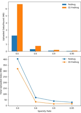
Figure 3 shows the compressed size of the MNIST-CNN updates for FedAvg and CE-FedAvg, including an uncom-pressed case (s = 0). It is interesting to see that while CE-FedAvg uploads more data per client per round (due to the extra variables from Adam) in all cases, the total data uploaded by CE-FedAvg is far lower than FedAvg in all cases. This is due to the large decrease in rounds to convergence CE-FedAvg gives.
Fig. 3. Top:Compressed uploaded data per client per round for FedAvg and CE-FedAvg with different sparsities, for the MNIST-CNNW= 40,C= 1.0,
Y = 2scenario.Bottom:Total uploaded data during training for the same scenario.
C. Testbed Setup
To test the real-time convergence of CE-FedAvg over FedAvg, we used a Raspberry-Pi (RPi) testbed to simulate a hetero-geneous low-powered edge-computing scenario. The testbed
consisted of 5 Raspberry Pi 2Bs and 5 Raspberry Pi 3Bs. A desktop acted as the server over a wireless network to emulate lower-bandwidth networking. The work of the server in these experiments was small: receiving and decompressing, aggregating and resending models to clients. Therefore, the server had a small impact on the time experiments took to run, and the vast majority of time taken in the FedAvg/CE-FedAvg algorithm was on the RPi clients. The RPi clients all had an install of Raspbian OS. Software was written with Python using Tensorflow 1.12.
Experiments with 10 workers, the MNIST-2NN and MNIST-CNN models, and sparsity rate s = 0.6 were per-formed to evaluate the runtime of CE-FedAvg and FedAvg. Round times were taken and averaged, and then used with the total-rounds from the relevant parts of Table I to determine the total time that experiment would take on the testbed. Time taken to complete rounds was very consistent on the testbed, making this a reliable estimator of total time.
D. Testbed Results
We ran experiments to get the estimated real time on a RPi testbed for a set of 4 experiments to reach given target accuracies. The results of this are shown in Figure 4.
Fig. 4. Estimated time on Raspberry Pi testbed of different FL scenarios.
The times in Figure 4 show that CE-FedAvg is able to converge to a given target accuracy in less real time than FedAvg with similar compression. Although the time taken per round is greater for CE-FedAvg than FedAvg (due in small extra computation required from Adam, but mostly due to the increased communication per round compared to similarly compressed FedAvg), the number of rounds taken to converge, as per Table I, was lower in all the given experiments. Figure 4 shows CE-FedAvg was able to converge 1.2−1.7×faster than FedAvg.
VI. CONCLUSION
Federated Learning (FL) can allow distributed Machine Learn-ing to be performed on the network edge usLearn-ing data gen-erated by IoT devices. We adapted FedAvg (a popular FL
algorithm) with Adam optimisation and compression to pro-duce Communication-Efficient FedAvg (CE-FedAvg), which reduces total uploaded data and rounds compared to similarly compressed FedAvg. Extensive experiments on the MNIST and CIFAR-10 datasets showed CE-FedAvg was generally able to reach a target accuracy in far fewer communication rounds than FedAvg in non-IID settings (up to 6× fewer). These experiments showed CE-FedAvg is also far more robust to aggressive compression of uploaded data, and able to converge with up to 3× less total uploaded data per client. Further experiments using a Raspberry-Pi testbed showed CE-FedAdam could converge in up to 1.7× less real-time. CE-FedAvg therefore presents the benefits of being able to train a model in less communication rounds (reducing the overall data and computing cost of training), less real-time, and with less uploaded data than uncompressed FedAvg, a unique result considering most schemes using compression reduce uploaded data at the cost of more rounds to convergence. Future work in this area could investigate other SGD-type algorithms applied to FL, and in compressing the models downloaded by clients from the server.
ACKNOWLEDGEMENT
This work was supported by EPSRC DTP Studentship. REFERENCES
[1] K. L. Lueth, “State of the iot 2018: Number of iot devices now at 7b - market accelrating,” August 2018. [Online]. Available: iot-analytics.com/state-of-the-iot-update-q1-q2-2018-number-of-iot-devices-now-7b/
[2] H. B. McMahan and D. Ramage, “Federated learning: Collaborative machine learning without centralized training data,” Google, April 2017. [Online]. Available: https://ai.googleblog.com/2017/04/federated-learning-collaborative.html
[3] H. B. McMahan, E. Moore, D. Ramage, and B. A. y Arcas, “Federated learning of deep networks using model averaging,” arXiv preprint arXiv:1602.05629, 2016.
[4] A. Hard, K. Rao, R. Mathews, F. Beaufays, S. Augenstein, H. Eichner, C. Kiddon, and D. Ramage, “Federated learning for mobile keyboard prediction,”arXiv preprint arXiv:1811.03604, 2018.
[5] S. Ramaswamy, R. Mathews, K. Rao, and F. Beaufays, “Federated learning for emoji prediction in a mobile keyboard,” arXiv preprint arXiv:1906.04329, 2019.
[6] J. Duchi, E. Hazan, and Y. Singer, “Adaptive subgradient methods for online learning and stochastic optimization,” Journal of Machine Learning Research, vol. 12, pp. 2121–2159, 2011.
[7] T. Tieleman and G. Hinton, “Coursera: Neural networks for machine learning,” Tech. Rep., 2012.
[8] D. Kingma and J. Ba, “Adam: A method for stochastic optimization,”
International Conference on Learning Representations, pp. 1–13, 2014. [9] Y. Zhao, M. Li, L. Lai, N. Suda, D. Civin, and V. Chandra, “Federated
learning with non-iid data,”arXiv preprint arXiv:1806.00582, 2018. [10] S. Wang, T. Tuor, T. Salonidis, K. Leung, C. Makaya, T. He, and
K. Chan, “Adaptive federated learning in resource constrained edge com-puting systems,”IEEE Journal on Selected Areas in Communications, vol. 37, no. 6, pp. 1205–1221, 2019.
[11] J. Koneˇcn´y, H. B. McMahan, F. X. Yu, P. Richtarik, A. T. Suresh, and D. Bacon, “Federated learning: Strategies for improving communication efficiency,”NIPS Workshop on Private Multi-Party Machine Learning, 2016.
[12] F. Sattler, S. Wiedemann, K. M¨uller, and W. Samek, “Sparse binary compression: Towards distributed deep learning with minimal commu-nication,”2019 International Joint Conference on Neural Networks, pp. 1–8, 2018.
[13] Y. Lin, S. Han, H. Mao, Y. Wang, and B. Dally, “Deep gradient compression: Reducing the communication bandwidth for distributed training,”International Conference on Learning Representations, 2018.
[14] F. Sattler, S. Wiedemann, K. M¨uller, and W. Samek, “Robust and communication-efficient federated learning from non-iid data,”arXiv preprint arXiv:1903.02891, 2019.
[15] S. Golomb, “Run-length encodings (corresp.),”IEEE Trans. Inf. Theor., vol. 12, no. 3, pp. 399–401, Sep 2006.
[16] Y. Chen, X. Sun, and Y. Jin, “Communication-efficient federated deep learning with asynchronous model update and temporally weighted aggregation,”arXiv preprint arXiv:1903.07424, 2019.
[17] L. Liu, J. Zhang, S. H. Song, and K. B. Letaief, “Edge-assisted hierarchical federated learning with non-iid data,” arXiv preprint arXiv:1905.06641, 2019.
[18] D. Leroy, A. Coucke, T. Lavril, T. Gisselbrecht, and J. Dureau, “Fed-erated learning for keyword spotting,” ICASSP 2019 - 2019 IEEE International Conference on Acoustics, Speech and Signal Processing (ICASSP), pp. 6341–6345, 2019.
[19] C. Liu, Y. Cao, Y. Luo, G. Chen, V. Vokkarane, M. Yunsheng, S. Chen, and P. Hou, “A new deep learning-based food recognition system for dietary assessment on an edge computing service infrastructure,”IEEE Transactions on Services Computing, vol. 11, no. 2, pp. 249–261, 2018. [20] H. Li, K. Ota, and M. Dong, “Learning iot in edge: Deep learning for the internet of things with edge computing,”IEEE Network, vol. 32, no. 1, pp. 96–101, 2018.
[21] L. Lyu, J. C. Bezdek, X. He, and J. Jin, “Fog-embedded deep learning for the internet of things,”IEEE Transactions on Industrial Informatics, vol. 15, no. 7, pp. 4206–4215, 2019.
[22] D. Reina, H. Tawfik, and S. Toral, “Multi-subpopulation evolutionary al-gorithms for coverage deployment of uav-networks,”Ad Hoc Networks, vol. 68, pp. 16–32, 2018.
[23] R. K. Pathinarupothi, P. Durga, and E. S. Rangan, “Iot-based smart edge for global health: Remote monitoring with severity detection and alerts transmission,”IEEE Internet of Things Journal, vol. 6, no. 2, pp. 2449– 2462, 2019.
[24] P. S. Chandakkar, Y. Li, P. L. K. Ding, and B. Li, “Strategies for re-training a pruned neural network in an edge computing paradigm,”2017 IEEE International Conference on Edge Computing, pp. 244–247, 2017. [25] Y. Shuochao, Z. Yiran, Z. Aston, S. Lu, and A. Tarek, “Deepiot: Compressing deep neural network structures for sensing systems with a compressor-critic framework,”Proceedings of the 15th ACM Conference on Embedded Network Sensor Systems, pp. 4:1–4:14, 2017.
[26] H. Guo, S. Li, B. Li, Y. Ma, and X. Ren, “A new learning automata-based pruning method to train deep neural networks,”IEEE Internet of Things Journal, vol. 5, no. 5, pp. 3263–3269, 2018.
[27] Y. LeCun and C. Cortes, “Mnist handwritten digit database,” 2010. [Online]. Available: http://yann.lecun.com/exdb/mnist/
[28] A. Krizhevsky, “Learning multiple layers of features from tiny images,” Tech. Rep., 2009.
[29] M. Abadi, A. Agarwal, P. Barham et al., “Tensorflow: Large-scale machine learning on heterogeneous systems,” 2015, software available from tensorflow.org.
Jed Mills is a Computer Science Ph.D. student in the College of Engineering, Maths and Physical Science at the University of Exeter, UK. He received a B.Sc. in Natural Science from the University of Exeter in 2018. His research interests are in machine learning, distributed machine learning and mobile edge computing.
Jia Hu is a Lecturer in Computer Science at the University of Exeter. He received his Ph.D. de-gree in Computer Science from the University of Bradford, UK, in 2010, and M.Eng. and B.Eng. degrees in Electronic Engineering from Huazhong University of Science and Technology, China, in 2006 and 2004, respectively. His research interests include cloud and edge computing, resource op-timization, applied machine learning, and network security.
Geyong Min is a Professor of High Performance Computing and Networking in the Department of Computer Science within the College of Engineer-ing, Mathematics and Physical Sciences at the Uni-versity of Exeter, United Kingdom. He received the PhD degree in Computing Science from the University of Glasgow, United Kingdom, in 2003, and the B.Sc. degree in Computer Science from Huazhong University of Science and Technology, China, in 1995. His research interests include future Internet, computer networks, wireless communica-tions, multimedia systems, information security, high-performance computing, ubiquitous computing, modelling and performance engineering.