A semi-supervised approach for the semantic
segmentation of trajectories
Soares J´unior A.
∗, Times V. C.
†, Renso C.
‡, Matwin S.
∗and Cabral L. A. F.
§∗
Dalhouise University (Canada)
†Federal University of Pernambuco (Brazil)
‡ISTI-CNR (Italy)
§Federal
University of Para´ıba (Brazil)
Abstract—A first fundamental step in the process of analyzing movement data is trajectory segmentation, i.e., splitting trajecto-ries into homogeneous segments based on some criteria. Although trajectory segmentation has been the object of several approaches in the last decade, a proposal based on a semi-supervised approach remains inexistent. A semi-supervised approach means that a user labels manually a small set of trajectories with meaningful segments and, from this set, the method infers in an unsupervised way the segments of the remaining trajecto-ries. The main advantage of this method compared to pure supervised ones is that it reduces the human effort to label the number of trajectories. In this work, we propose the use of the Minimum Description Length (MDL) principle to measure homogeneity inside segments. We also introduce the Reactive Greedy Randomized Adaptive Search Procedure for semantic Semi-supervised Trajectory Segmentation(RGRASP-SemTS) algorithm that segments trajectories by combining a limited user labeling phase with a low number of input parameters and no predefined segmenting criteria. The approach and the algorithm are pre-sented in detail throughout the paper, and the experiments are carried out on two real-world datasets. The evaluation tests prove how our approach outperforms state-of-the-art competitors when compared to ground truth.
Index Terms—Trajectory segmentation; Semantic annotation; Semantic trajectory; Semi-supervised learning.
I. INTRODUCTION
Research on trajectory management and analysis is a broad and mature area [16] since positioning devices are now com-monly used to track people, vehicles, vessels, and animals. These devices produce trajectory samples representing the object movement as a discrete collection of spatiotemporal points, or samples. An important step that is a prerequisite to several analysis tasks on these tracks is the trajectory segmentation[14, 17]. Segmenting a trajectory means splitting the spatiotemporal sequence of points into segments based on some properties or criteria that identify a similar behavior in the segment. Examples of segment splitting criteria are based on the temporal component like the day of the week or based on whether the object is moving or not, thus identifying the stop segments from the move segments [17]. Segmenting a trajectory with clear criteria is a first step to semantically enrich trajectories (or semantic annotation), a process to enrich trajectory parts with meaningful contextual information [14, 12].
The segmentation task is therefore based on methods ca-pable of distinguishing the homogeneous or similar parts of a trajectory based on some criteria. We can distinguish two
cases: supervised and unsupervised segmentation. In super-vised segmentation, the criteria are already known a priori. This can be implemented with algorithms based on simple thresholds (e.g., speed) or machine learning techniques that learn the correct segmentation from a set of labeled segments. When the segmentation criteria are unknown, the unsupervised algorithm derives the homogeneity of segments based on some cost function. Both supervised and unsupervised methods have complementary benefits and drawbacks. The supervised meth-ods rely on user-defined rules, labels or thresholds; therefore the segmentation is user-driven. This kind of segmentation is particularly suitable for semantic annotation, thanks to the human labeling phase that can associated complex semantic labels to trajectory parts (e.g. activity performed or transporta-tion means). The drawback is that, in some cases, these criteria are not clear, they may depend on the characteristics of the trajectory dataset and the expertise of the domain specialist to correctly label a set of trajectories and/or configure the thresholds. Also, obtaining a high quality labeled trajectory dataset is difficult as it relies on a huge effort by domain experts and this is one reason why the supervised methods are not widespread in this field.
Unsupervised algorithms, on the contrary, avoid any control from the user and automatically detect segments using a cost function which represents the homogeneity of the segments. Although these algorithms can produce segments with high homogeneity, they lack semantics and any connection to the specific application, making the interpretation task difficult. Despite the broad spectrum of trajectory segmentation ap-proaches already proposed in the literature (see for example [16, 14]), there is still a lack of methods attempting to combine the benefits of both supervised and unsupervised strategies. As a possible solution to this, a semi-supervisedapproach to the segmentation task is proposed in this work.
Semi-supervised means essentially that a user labels man-ually a small set of trajectories based on some criteria, thus giving the semantics of the segmentation and, from that, the method infers, in an unsupervised way, the segmentation of the remaining part of the trajectory dataset. Such approach offers a balance between methods which are entirely supervised, where the user precisely defines the splitting criteria, and unsupervised, where the method infers a good splitting based on a cost function. We observe that when the segmentation is semantic-based (e.g., representing the activity of the moving object), in contrast to the geometric-based segmentation (e.g., the speed of the object), the need for manually annotated
trajectories is crucial: minimizing the number of these human-labeled trajectories, as stated in [8], is fundamental to keep this task feasible.
This paper comes as advancement and extension of a previous work [7] based on an unsupervised method named GRASP-UTS (Greedy Randomized Search Adaptive Search Procedure for Unsupervised Trajectory Segmentation). Com-pared to that paper, which introduces an unsupervised algo-rithm for trajectory segmentation, here we propose a new semi-supervised segmentation algorithm called RGRASP-SemTS (Reactive Greedy Randomized Adaptive Search Procedure for Semantic semi-supervised Trajectory Segmentation).
We summarize below the original contributions of this paper:
• Proposal of the RGRASP-SemTS as a semi-supervised algorithm to segment trajectories that uses a small set of labeled trajectory data during the trajectory segmentation task to drive the unsupervised segmentation of unlabeled trajectory data.
• Unlike previous related works, RGRASP-SemTS focuses
on performing semantic trajectory segmentation using features evaluation, non-monotone criteria, semantic an-notation, cost function and meta-heuristics.
• Description of a feature evaluation step that aims to find the best set of features for increasing the RGRASP-SemTS’s performance.
• Proof that using labeled data helps speeding up the RGRASP-SemTS’s performance when compared to our previous unsupervised algorithm, GRASP-UTS.
• Description of experiments with two real world datasets showing that the performance of RGRASP-SemTS is superior when compared to other unsupervised and su-pervised approaches of the literature.
The remainder of the paper is organized as follows. Sec-tion II surveys the related work. SecSec-tion III shows con-cept definitions, terminologies, and theories used in the proposed solution. Section IV presents the novel semantic semi-supervised algorithm for trajectory segmentation named RGRASP-SemTS. Section V presents the metrics and the results obtained by the novel approach when applied to real datasets. Finally, Section VI concludes the paper.
II. RELATEDWORKS
As the interest in the literature is increasing, new methods to segment trajectories are being proposed. Pioneering work is thestop and movedefinition given by [17] where the segmen-tation was used to identify the parts of the trajectories where the object stays still and separate it from the moving parts. We later come to a broader definition of semantic trajectory, where the segments may identify and be annotated not only asstops and moves, but also with more meaningful andcontext-aware labels such as transportation means or activities [2, 14, 12]. The need to identify segments based on some semantics fostered the developments of different segmentation methods. A possible classification of these methods is based on the characteristics of the algorithm: supervised or unsupervised, application-oriented or general purpose, monotone criteria
or non-monotone criteria and with a predefined number of segments versus a non-predefined number of segments.
Supervised means that the segmentation criteria are based on ad-hoc standards and predefined rules. This is the case when the rules are clear and predefined by experts of the domain as in works [13, 11, 20]. The second line of approaches follows an unsupervised methodology, where no predeter-mined criteria are imposed in the segmentation process, and the segment split is based on data properties as in works [9, 18, 7]. To the best of our knowledge, no works found in the trajectory segmentation literature tried to combine both supervised and unsupervised criteria as we are doing in the present paper.
Another possible classification of segmentation algorithms is to distinguish between application-oriented and general purpose methods [9]. Application-oriented algorithms for tra-jectory segmentation are designed for a specific purpose and, consequently, they are difficult to reuse in different domains. Examples of application-oriented algorithms for trajectory segmentation are described in [18, 19, 20]. On the other hand, the general purpose algorithms for trajectory segmentation are easily reused in many different domains. Examples of general purpose algorithms for trajectory segmentation are explained in [4, 7, 9, 13, 11]
Trajectory segmentation algorithms can also be monotone or non-monotone, and this affects the results of the splitting task [4]. Indeed, a criterion is monotone if any sub-segment S0 of a segmentSalways fulfills the whole segment criterion. Monotone criteria are found when values of the features fall within a range or ratio. On the other hand, values computed from means and standard deviations are non-monotone. Trajec-tory segmentation algorithms with monotone criteria includes works [4, 1], while the approaches with non-monotone criteria include [9, 13, 11, 7, 20]
Another issue related to the segmentation of trajectories is the number of segments that must be found. In [9], the number of segments is given as input to the algorithm, so it is already predefined, whereas, in [7, 13, 11, 20], the number of segments is found automatically by the algorithm during its execution.
The RGRAPS-SemTS algorithm proposed in this paper is classified as being semi-supervised, general purpose, non-monotone and lacking a predefined number of segments. To the best of our knowledge, none of the segmentation algorithms proposed in the literature has such classification.
III. BASIC CONCEPTS
This section addresses concepts and terminologies used in this work. A trajectory is a representation of the spatiotemporal movement of an object. Trajectories are usually collected by tracking devices into discrete samples and represented as a sequence of spatiotemporal points [7]:
Definition 1:Atrajectory sampleis a list of spatiotemporal pointsτN ={tp0, tp1, . . . , tpN}, where tpi = (xi, yi, ti, ωi).
Apoint feature(ωi in Definition 1, is a set ofpoint features with ωi = {pf0, pf1, . . . , pfA}) is any numeric information that can be extracted from a trajectory sample and associated to a spatiotemporal point. A point feature can be acquired
by a geolocation device (e.g., the instantaneous speed) or calculated using the trajectory sample (e.g., the direction variation between two consecutive points) and is assigned to a single point of the trajectory.
A segment feature is any numeric information computed from the trajectory sample and associated with a segment (e.g., average or maximal speed). The difference betweenpoint featureandsegment featureis that, while the former is static, the latter is more dynamic. Once a point feature information is collected or computed it will not change over time. The segment features depend on the segment definition and when the segment is recomputed by adding or removing points, then the segment feature has to be recomputed too.
Asemantic label(or semantic annotation) is any additional semantic and/or contextual information that can be added to a trajectory segment [14]. Such information can be, for example, an activity (e.g., walking, studying or driving) or a behavioral pattern (e.g., foraging or running from a predator). Henceforth, the term label refers to asemantic label. A trajectory dataset is called a labeled dataset when its trajectories’ segments have been annotated with semantic labels. More formally:
Definition 2: A labeled trajectory segment s is a sublist of τ and s = (tid, sid,{tpu, . . . , tpv},semantic label, ζsid), where: (i)tidis the trajectory identifier; (ii)sidis the segment identifier; (iii) tpu, . . . , tpv represent a sublist of τN starting from tpu and ending at tpv (1 ≤ u ≤ v ≤ N); (iv)
semantic labelis the additional information that characterizes the segment and (v) ζsid is a list of segment features, with ζsid={sf0, sf1, . . . , sfB}.
Two more concepts are used in the segmentation algorithm definition to refer to the representative points inside a seg-ment and inside a labeled dataset: the segment landmark in Definition 3, already introduced in [7] andsemantic landmark in Definition 4, introduced here for the first time:
Definition 3: A segment landmark lmr is a representative point of a trajectory sample τN, where lmr = tps and 1 ≤
r ≤s ≤N, used to represent a trajectory segment in terms of its point features.
A segment landmark is a point inside the segment that is chosen to represent the whole segment: it is used as reference point to characterize the behavior of a part of the trajectory. After defining a set of segment landmarks, it is possible to create segments by partitioning the points in the neighborhood where each segment landmark is defined (i.e. the trajectory’s consecutive points respecting a time constraint). The decision of which point to choose as a segment landmark depends on a cost function that should be optimized.
Definition 4: A semantic landmark sem lm = (semantic label, ωA, ζB) is a set that represents a pattern extracted from a labeled dataset consisting of: (i) a semantic label; (ii)ωA is a list ofpoint featuresvalues; and (iii) a list ζB ofsegment features values.
Differently fromsegment landmarksthat are decided by the cost function, thesemantic landmarksare computed from a set of examples given by the user. Example ofsemantic landmarks are segments labeled as fishing or not fishing for vessels or foraging andtravelingfor animals.
IV. SEMANTIC AND SEMISUPERVISED TRAJECTORY SEGMENTATION
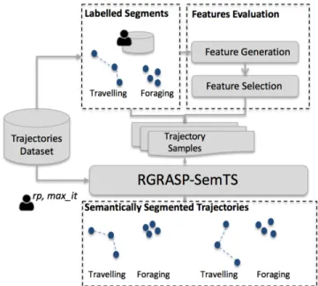
This section introduces the novel RGRASP-SemTS process for semantic and semi-supervised trajectory segmentation. This process is summarized in Figure 1 where we specify the process tasks and their input and output. Starting with a set of trajectories, the domain expert labels a subset of them using some criteria (e.g., the activity performed). The first step of the process is the features evaluation step where the features that will be used in the learning phase are generated and selected for a particular domain. This step is detailed later in Section IV-A. The second task is the actual segmentation performed by RGRASP-SemTS. The input parameters of RGRASP-SemTS are: (i) a set of labeled segment examples; (ii) a reactive proportion (rp) to update internal list of parameters values for minT ime andα, and (iii) the maximal number of itera-tions (max it) to execute RGRASP-SemTS over a trajectory sample. This algorithm and the input parameters are detailed in Section IV-B. Finally, the output of RGRASP-SemTS is a set of semantically segmented trajectories produced in a semi-supervised way by considering both the examples provided by the user (supervised phase) and the similarities computed by the algorithm in the neighborhood of the segments (unsuper-vised phase).
Fig. 1. The semantic and semi-supervised trajectory segmentation process of RGRASP-SemTS
A. Feature evaluation
The feature evaluation follows two steps: (i) the feature generation and (ii) the selection of a subset of features enabling the algorithm to achieve its best performance. In the features generation step, the objective is to create as many features as possible to characterize the behavior of the moving object for each dataset. The features created for each dataset used in the experiments of this work are detailed in Section V-B.
As the number of features can grow very fast, it is necessary to select the most representative point and segment features
to perform the segmentation, and this is the second step of features evaluation. In this work, the Weka package and the filteringχ2algorithm [10] were used to select the features. The χ2feature selection algorithm evaluates the value of a feature
by computing the value of theχ2statistic concerning the label.
The advantages of this method are that it is fast, scalable and independent from the chosen segmentation algorithm. B. The RGRASP-SemTS Segmentation Algorithm
Semi-supervised strategies take advantage of both unsuper-vised and superunsuper-vised strategies, thus exploiting labeled and unlabeled data. In fact, we want to achieve homogeneity inside a segment using an unsupervised strategy (segment landmarks), while obtaining a degree of similarity between the segments using a supervised strategy on a labeled dataset ( se-mantic landmarks). The properties we want to optimize in the segments (e.g.,minimal distortionandmaximal compression), previously presented in [7], and the extended cost functions we use in this work are discussed below.
1) Desirable properties and Cost function definition: In this work, achieving minimal distortion in a trajectory segmen-tation task is to achieve as much homogeneity as possible inside the trajectory segments regarding its pointandsegment features. On the other hand, achieving maximal compression for the trajectory segments means that the resulting segments (i.e. number of segment landmarks) should be as few as possible and as similar as possible to a semantic landmark extracted from the labeled dataset.
The concepts ofmaximal compressionandminimal distor-tion are inversely correlated since when one increases, the other decreases. For example, selecting all the spatiotemporal points as segment landmarks naturally decrease the minimal distortion increasing the maximal compression since many segment landmarks will be chosen. Conversely, choosing one point as a segment landmark for the entire trajectory lowers maximal compression, but increases the distortion produced by the segmentation since a single segment landmark will be compared to all the points of the trajectory. As these concepts are inversely correlated, it is necessary to define a function that represents the trade-off between them. We propose to use the MDL principle to compute this trade-off as detailed below. To achieve homogeneity inside a trajectory segment we use Equation 1 which represents a Euclidean distance between the trajectory point features (ωA) of two points tp1 and tp2. In
Equation 1, ω1i represents thei-th point feature value oftp1
andω2i the i-th point featurevalue oftp2.
simtf(ω, ω) = v u u t A X i= (ωi−ωi) (1) The segment cohesiveness is shown in Equation 2 and measures the similarity between thepoint featuresof a chosen segment landmarkωlm and all the points betweentpuandtpv (ωk). S Cohe(ωlm,{ωu, . . . , ωv}) = v X k=u simtf(ωlm, ωk) (2)
Assegment feature is a new concept defined in this work and as it is necessary to compare the segment features of different segments, Equation 3 defines a similarity between thesegment features(ζ) of two segmentss1ands2, whereζ1i
represents thei-th segment featureofs1andζ2irepresents the
i-th segment feature ofs2.
simsf(ζ1, ζ2) = v u u t B X i=1 (ζ1i−ζ2i) 2 (3)
In the MDL theory, the best model is the one that minimizes the result ofL(H) +L(D|H)[5]. In this work, the hypothesis H consists of choosing an optimal set of segment landmarks that are more similar to thesemantic landmarksincluded in the labeled dataset and also contains high homogeneity rates in its neighborhood. Finding the optimal set of segment landmarks reflects the decision of finding the best hypothesis according to the MDL principle. It is crucial also to consider the use of unsupervised and supervised data in bothL(H)andL(D|H). Given a trajectory sample τN = (tp, tp, ..., tpN), a set of segment landmarks φT ={lm, lm, ..., lmT}, a set of
semantic landmarks λV ={s lm, s lm, ..., s lmV}, and a set of trajectory segments θT ={s, s, ..., sT}, the cost function is formally defined as follows.
The cost of the hypothesis (L(H)) is computed by compar-ing, regarding their point features: (i) the chosen consecutive segment landmarks (unsupervised measure); and (ii) each segment landmark to the most similar semantic landmark found in the labeled dataset (supervised measure). Equation 4a represents the cost of encoding a hypothesis of atrajectory sample τN when a setφT of segment landmarks are chosen. IfT is equal to 1,L(H) = 0. Otherwise, Equation 4a is used. Themaxrepresents the maximum possible similarity between two trajectory features. The first part of Equation 4a repre-sents the unsupervised measure (Equation 4b) that takes into account the unlabeled data. This value will decrease when the consecutively chosensegment landmarksare dissimilar; hence, this Equation identifies less similar movement behaviors by comparing the current segment to the next one. The second part of the L(H) function (Equation 4c), which stands for the supervised measure, computes the similarity between the chosen segment landmark and the closest semantic landmark regarding their point features.
L(H) =U ns L(H)(φT) +Sup L(H)(φT, λV) (4a) U ns L(H) = log2(1 + T−1 X j=1 max−simtf(ωlmj, ωlmj+1)) (4b) Sup L(H) = log2(1 + T X j=1 arg min i∈[1,V]simtf(ωlmj, ωs lmi)) (4c)
The L(D|H) cost function, representing the cost of bits for encoding a dataset D when testing a hypothesis H, is defined in Equation 5a. The cost of encoding a dataset given a hypothesis (L(D|H)) is computed by comparing: (i) the
segment cohesiveness (Equation 2) between all the points of each segment ({ωu, ..., ωv}k) and its respective segment
landmark(ωlmk) in terms ofpoint featuresvalues; and (ii) the
segment featuressimilarity (Equation 3) between each segment found and the more similar semantic landmark. The first part of Equation 5a is the unsupervised measure (Equation 5b) that will compare the chosen segment landmark of each segment with all point features’values inside this segment. This value increases when fewer segments are found and decreases when more segments are found. The supervised measure of our L(D|H) is shown in Equation 5c. Each segment θT found is compared to all semantic landmarks of the set λV and the closest one is selected. This is the part of the cost function where semantic enrichment is performed. Since the unsupervised measure ofL(D|H)(Equation 5b) compares all thepoint features’values of each segment with the respective segment landmark, it is necessary to multiply this similarity by the number of points located inside this segment (|sk|) and subtract one, since the segment landmark is a point of the segment and the similarity between them is equal to 0. If such approach is not adopted, theL(D|H)value will consider the unsupervised measure more costly when compared to the supervised measure since greater similarity costs would be computed. L(D|H) =U ns L(D|H)(θT) +Sup L(D|H)(φT, λV) (5a) U ns L(D|H) = log2(1 + T X k=1 SCohe(ωlmk,{ωu, . . . , ωv}k)) (5b) Sup L(D|H) = log2(1 + T X k=1 arg min i∈[1,V]simsf(ζsli, ζsk) ∗ |sk|) (5c)
2) The Algorithm: In this section, we present the algorithm RGRASP-SemTS. Two issues must be considered: (i) the number of segments that makes the cost function minimum is not known a priori; (ii) switching the segment landmarks implies that the segment configuration will also be affected, since the cost function value must be recomputed every time a modification in the set of segment landmarks is per-formed. To manage these issues, we adopt theReactive Greedy Randomized Adaptive Search Procedure (RGRASP) meta-heuristic[15], aiming at determining the number of segments and the boundaries between the consecutive segments.
RGRASP-SemTS is detailed in Algorithm 1. The trajectory τN to be segmented is read in Line 1. In Line 2, the algorithm extracts a semantic landmarkfor each type ofsemantic label that must be found by finding the average of each pointand segment feature contained in the segment examples consider-ing the semantic label. Lines 3 and 4 initialize minT imelist and αlist for possible values for minT ime and α using equal width binning. In the case of αlist, the minimum and maximum values are predetermined and range from 0.1 to 0.6. These values were determined because, for values below 0.1, the algorithm chooses the same segment landmarks in each iteration. For values above 0.6, the segment landmarks chosen by RGRASP-SemTS were completely random. From
Algorithm 1 RGRASP-SemTS
Input: A set of segment examplesψE= (ex1, ex2, ..., exT)
A reactive proportion value rp A number of iterations max it
Output: A set of semantically enriched segments θT = (s1, s2, ..., sT)
1: τN ⇐ read trajectory data;
2: λV ⇐extract all semantic landmarks from examplesψE; 3: minT imelist⇐initialize theminT imevalues;
4: αlist⇐initialize theαvalues; 5: fork= 1→max itdo
6: minT ime⇐randomly select from minT imelist; 7: α⇐randomly select fromαlist;
8: θT ⇐Greedy Randomized Construction Procedure(τ, minT ime,α,λV);
9: θT ⇐ Local Search Procedure(θT,minT ime,λV); 10: Update Best Solution(θT, BestθT);
11: ifmod(k, rp) == 0then
12: Update minT imelist andαlist probabilities; 13: end if
14: end for
returnBestθT;
Lines 5 to 14, max it iterations are executed aiming at building and evaluating different segmentations. Values forα andminT imeare randomly selected from the listsαlist and minT imelist (Lines 6 and 7). Then, a first feasible solution (θT segments) is built by executing the procedure shown in Algorithm 2 (Line 8). After building the first set of feasible segmentsθT, Local Search Procedure (Algorithm 3) is applied to optimize the segments (Line 9) locally. RGRASP-SemTS (Algorithm 1) verifies if the new set of optimized segments θT is the best one found by evaluating the cost according to the MDL function (Line 10). If the cost of these segments is lower, it updates the set of best segments (Best θT).
Thereactivepart of this algorithm is concluded by updating the probabilities ofminT imelist andαlist (Lines 11 to 13). If the modulo (mod) of the multiplication between it and rp is equal to 0, the probabilities ofαlist andminT imelist are updated using Equation 6 [15]. Equation 6 (a) deter-mines the probability of selecting a determined value of αlist or minT imelist. Equation 6 computes the values for pi (i.e. probability of selecting an element of the αlist or minT imelist) when all values for qi are established. This is achieved by dividing each value of qi by the total sum of all qis.
qi= (
best mdl value f ound
average mdl value f or ith element of the list)
10 (6a) pi=qi/ m X j= qj (6b)
Finally, Algorithm 1 returns the best set of semantically enriched segments (BestθT) found bymax ititerations. The procedure for building the initial solutions (Algorithm 2) of the RGRASP-SemTS is explained as follows.
Algorithm 2 Greedy Randomized Construction Procedure
Input: A set of points ordered by time τN = (tp1, tp2, ..., tpN)
A minimum time thresholdminT ime
An α threshold to define the amount of greediness of the construction algorithm
AλV set of semantic landmarks
Output: A set of semantically enriched segments θT = (s1, s2, ..., sT)
1: whilecandidatelist is not emptydo
2: RCLlist⇐add points ofcandidatelist from index 0 toRCLsize;
3: candidate ⇐randomly select a point fromRCLlist; 4: semanticLandmark⇐get the most similar semantic
landmark fromλV in terms of point features; 5: segment ⇐addcandidate;
6: while minT ime threshold condition not satisfieddo
7: best neighbor⇐evaluate left and right neighbor; 8: segment⇐best neighbor;
9: end while
10: θT ⇐addsegment;
11: remove fromcandidatelist unfeasible points; 12: sort points of candidatelist according to the closer
semantic landmark in terms of point features; 13: end while
returnθT;
Algorithm 2 starts in Line 1 by considering all points as can-didatesegment landmarks(candidatelist). In the initialization of all GRASP-based algorithms, the creation of a restricted candidate list (RCL) is necessary. This list is used to manage the amount of greediness of the initialization method that is determined by the parameter α. This procedure is executed until all points in candidateP ointslist are considered land-marks (Lines 2 to 15). In this work, the RCL is built by sorting all points insideτ according to its distance (Equation 1) to the closestsemantic landmarkregarding the point features values (Line 1). The size of the RCL (RCLsize) is determined by multiplying the size of the candidatelist by the value of α, thereby creating a variable RCLlist with all points spanning from the first element of the candidatelist to the position determined inRCLsize. Afterward, a point from theRCLlist is randomly chosen as candidatesegment landmark(Line 3) and the closest semanticLandmarkfor this point is chosen by computing the trajectory features distance (Equation 1) between this candidate and all semantic landmarks of the setψV (Line 4).
A new segmentis created in Line 5 with the initial point being the candidate and its semantic label being the one determined by thesemanticLandmark(Line 8). From Lines 6 to 9, the size of the segmentis increased by adding points to the segment’s neighborhood (respecting the chronological order) until the time threshold (minT ime) is reached. This is done by determining the most suitable neighbor in terms of point features’ values (i.e.segmentu−1 andsegmentv+1)
of the segment (Line 7) and adding this bestN eighbor to the segment (Line 8). When segment contains at least the
minT ime threshold, this segment is added to the set θT (Line 10). After, all points of the segment (Line 10) and the neighborhoods that could not be used to build a feasible segment regarding the time constraint (Line 11) are removed from the candidatelist. After removing all these points, the candidateP ointslist is re-sorted (Line 12), and the same procedure is applied until the there are no candidate points in this list. Subsequently, all points that were not assigned to a segment are placed in the neighbor segment (segment in the point’s right or left). From that point on, the algorithm detects which position, among a set of consecutive points that had not been assigned to a segment, is the best one - that is, the one which reduces the cost function. These points are then added to the respective segment (i.e., a segment on the left or the right) whose cost function was minimized. Finally, feasible and semantically enrichedθT segments are returned.
Algorithm 3 Local Search Procedure
Input: A set of semantically enriched segments θT = (s1, s2, ..., sT)
A minimum time thresholdminT ime AψV set of semantic landmarks
Output: A set of optimized semantically enriched segments optimized θR= (s1, s2, ..., sT)
1: optimized θR ⇐ {}; 2: c segment ⇐θ0;
3: p sem label ⇐c segmentlabel; 4: fori= 1→T do
5: ifp sem label !=θi’s semantic labelthen 6: update segment landmark ofc segment; 7: optimized θ ⇐addc segment; 8: p sem label ⇐c segmentlabel; 9: c segment⇐ θi;
10: else
11: current segment ⇐insert all points fromθi; 12: end if
13: end for
14: fori= 0→R−1 do
15: bpp ⇐ Find the best position to partition points betweenindexlm1 andindexlm2;
16: optimized θi⇐create segment fromoptimized θi’s first index position tobpp;
17: optimized θi+1 ⇐ create segment from bpp+ 1 to optimized θi+1’s last index;
18: update segment landmark of optimized θi and optimized θi+1;
19: end for
returnoptimized θR;
The procedure to locally optimize the initial solution (Algo-rithm 3) of the RGRASP-SemTS is explained as follows. Line 1 initializes a list of optimized segments namedoptimized θR that will be the output of this procedure. Lines 2 and 3 initialize the current segment (c segment) to be analyzed with all the points contained in θ0 and stores this segment’s
semantic label inp sem label.
The objective of lines from 4 to 13 is to merge segments with the samesemantic labels. For all the remaining segments
θT, if the consecutive labels (i.e., labels from the previous segment and the current) are not equal (Line 5), the algorithm updates thec segment’ssegment landmark(Line 6), adds this segment to the output list of segmentsoptimized θ (Line 7), sets the previoussemantic labelas the actual one in the current segment (Line 8), and finally setsc segmentas being equal to θi (Line 9). If the p sem labelis equal to theθi’s semantic label, all points from θi are added to the c segment (Line 10).
From Lines 14 to 19, Algorithm 3 optimizes the MDL based cost function L(H) +L(D|H). The optimization is carried out by finding the best partitioning position (bpp) between the consecutive segments on the set optimized θ (Line 15). This method verifies for all points between consecutive seg-ment landmarks, which one causes a sharper decrease in the MDL-based cost function result, and considers this position as the local optimum for these successive segments. The optimized θi and optimized θi+1 boundaries in Lines 16
and 17 are updated, as well as their segment landmarks in Line 18. Finally, a set of optimized θR is returned by this procedure.
Since RGRASP-SemTS works with distances, the stan-dardization of the data is a crucial step because features can have different variances. Indeed, when there is a feature with a very high variance, the distances computed between the features will be greater than the distances computed for features with smaller variances. This difference would impact the RGRASP-SemTS by raising the cost of the features with higher variances and decreasing the cost of features with lower variances. In this work, each feature was normalized using the well-known statistical method known as standard score. This method produces a dimensionless number that is obtained by subtracting a raw value from the mean and then, dividing this difference by the standard deviation.
At this point, the complexity analysis of the RGRASP-SemTS is explained. The complexity of the construction procedure (Algorithm 2) is defined by thewhilestructure from Lines 2 to 17. This structure has a complexity of O(N), and it evaluates, for each point from the trajectory τN, the possibility of it being selected as a segment landmark. When these lines are executed, every time a new segment is created, points from the list of candidate points (candidateP ointslist) are removed in Lines 14 or 15. At maximum, all the points from trajectory τN could be selected as segment landmarks to generate segments. The complexity of the local optimiza-tion procedure (Algorithm 3) is defined by the for structure from Lines 13 to 21. Observe that the θR segments evalu-ated by Algorithm 3 contain all the points from τN. Note also that all the possibilities for partitioning the N points between two consecutive segment landmarks are analyzed, determining a complexity of O(N)for Algorithm 3. Finally, the RGRASP-SemTS (Algorithm 1) complexity is defined as O(N ∗max it). It results from the multiplication of Lines 7 or 8 and the number of iterations the algorithm executed (max it), since all the previous Lines of this algorithm have lower complexities.
V. EXPERIMENTS
This section details the experiments performed in this work and is organized as follows. Section V-A presents the datasets and evaluation metric, while Section V-B details the features evaluation. Finally, Section V-C compares the semantically enriched segments generated by RGRASP-SemTS with other state-of-the-art supervised and unsupervised algorithms. A. Datasets and evaluation metric
We used two real world datasets: (i) the Atlantic hurricane track dataset and (ii) tracked grey seals dataset.
The Atlantic hurricane track dataset1 contains information regarding hurricanes collected from 2000 to 2012 and it was divided into segments labeled low intensity hurricanes (e.g., surface wind ≤63knots) and high intensity hurricanes (e.g., surface wind > 64 knots). Trajectories with less than 20 points were discarded to avoid the segmentation of very small trajectories and because most of them only contained the semantic label low intensity.
The grey seals dataset contains information regarding seals’ trajectories collected from Argos satellite tags deployed from Sable Island, Nova Scotia, Canada. This dataset contains segments with labels foraging and traveling, assigned by domain specialists [3].
In the experiments we evaluate the segments generated by the segmentation algorithms using the Area Under the Curve (AUC) of the Receiver Operating Characteristic (ROC) analysis. Thesemantic labelwas registered for eachtrajectory pointof all datasets with the ground truth in the datasets used in the experiments. The ground truth is the data classification stored in the database by domain specialists, and it is used to validate the segmentation results. This validation aims at verifying if the assignment of thesemantic labelto each point of the segment done by a segmentation algorithm is correct. Thanks to this information, it is possible to build the confusion matrix of the ROC analysis and compute the AUC.
B. Features evaluation tests
The first step of the features evaluation is the features generation. This step is very important for RGRASP-SemTS because many point and segment features can be generated from trajectory raw data and relevant features are unknowna priorifor a given domain. The key idea is to generate a large set ofpoint and segment featuresand verify in a subsequent step which of them better characterizes asemantic label.
For the hurricanes dataset, we generated aspoint features: the maximum sustained surface wind at six-hour intervals, the estimated speed in meters per second and the direction variation between points from 0 to 180 degrees. Forsegment features, we computed: average, minimum and maximum values of surface wind, estimated speed, and direction, the ground distance between the first point and the last point of the segment and the elapsed time for each segment. For the grey seals dataset, the point features extracted were the depth, the distance from the shore in km, and a binary column
indicating whether the seal was near the shore using a distance threshold of 15km, estimated speed, and direction variation. For segment features, we computed: average, minimum and maximum values of all the 5 point features and the ground distance between the first point and the last point of the segment and the elapsed time for each segment.
Finally, for the features selection we used the feature rank-ing methodχ2[10] implemented in the Weka [6] package. We
selected the best set of features, by analyzing the RGRASP-SemTS’s performance in terms of AUC values. In particular, five trajectories were randomly selected, and their segment features were extracted. Sequentially, an ARFF file (the Weka input format) was generated, containing the acquired infor-mation. It is worth noticing that we used here only segment features due to a Weka package limitation since this software only allows the representation of each labeled segment as a single example. The χ2 algorithm has been executed, and stored the rank of each segment feature. Subsequently, we executed RGRASP-SemTS with the maximum number of features, and stored the AUC value. Finally, the last ranked segment feature from theχ2was removed and the AUC value
measured once again. The procedure was repeated until only one segment feature remained.
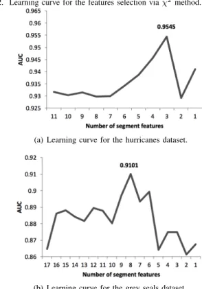
Figures 2(a) and 2(b) show the AUC performance of the RGRASP-SemTS using this approach. It is worth noticing that, for the hurricane dataset, 3 segment features (e.g., average, minimum and maximum surface wind) have generated the best result in terms of AUC value (0.9545). For the grey seals dataset, 8 segment features (e.g., average, maximum and minimum direction variation, maximum and minimum speed and the distance between the first and last point of the segment) have produced the best AUC performances, which was0.9101. Based on these results, the decision was to use threesegment features and thepoint feature surface wind for the hurricane dataset. For the grey seals dataset, the decision was to use the eight segment featuresand the estimated speed and direction variation as point features.
C. Evaluating RGRASP-SemTS
This section evaluates the performance of the RGRASP-SemTS when compared to other approaches from the liter-ature. Section V-C1 compares RGRASP-SemTS’s execution time to the unsupervised approach GRASP-UTS. Finally, in Section V-C2, the performance of RGRASP-SemTS is com-pared with other state-of-art algorithms.
1) Runtime analysis of RGRASP-SemTS: In this section we evaluate the execution time of RGRASP-SemTS by comparing with the unsupervised version GRASP-UTS. The objective is to show how the information provided by the user improves the execution time when compared to the unsupervised GRASP-UTS. In this experiment, one trajectory of each dataset was randomly selected, and both the RGRASP-SemTS and the GRASP-UTS were executed one hundred times (100 iter-ations). A minT ime value was used for both algorithms (12 hours for both datasets), and a full search (partitioning factor input parameter for GRASP-UTS) was ensured for both algorithms.
Fig. 2. Learning curve for the features selection viaχ2method.
(a) Learning curve for the hurricanes dataset.
(b) Learning curve for the grey seals dataset
Figure 3(a) and Figure 3(b) summarize the results. For the hurricanes dataset, on average, the RGRASP-SemTS was 0.064 seconds faster than GRASP-UTS, while it was 6.7 seconds faster for the grey seals dataset. After one hundred iterations, it is possible to notice that 1 second was saved for executions of the hurricane dataset and 600 seconds were saved for the grey seal dataset. It is important to observe that this difference is probably because the hurricanes’ trajectories are smaller in point length (between 80 and 140 points), while the grey seals’ trajectories contain more points to be evaluated (each trajectory contains more than 1000 points).
Although RGRASP-SemTS and GRASP-UTS have the same complexity O(N ∗ max it), the runtime difference between them is a result of the necessary time for the GRASP-UTS to re-build all the solution when landmarks are modified (i.e. inserted, removed or had positions switched). Since RGRASP-SemTS uses some information provided by the user, fewer modifications in the segments are made when an iteration is executed.
2) Comparison of RGRASP-SemTS with state-of-art al-gorithms: This section presents a performance comparison assessed in terms of AUC between RGRASP-SemTS and other state-of-art unsupervised (GRASP-UTS [7] and WK-Means [9]) and supervised (e.g., CB-SMoT [11] and SPD [20]) segmentation algorithms.
The objective was to evaluate the performance of the algorithms when only small amount of data are available for training therefore we limit the analysis to one sub-dataset. We divided both the hurricanes and grey seals dataset into 10 subsets.
Fig. 3. Execution time analysis of RGRASP-SemTS
(a) Time analysis for the hurricanes dataset.
(b) Time analysis for the grey seals dataset
as input for the segment landmarks the labeled examples con-tained in thetraining set. For the other algorithms, parameters’ values estimated in the training set were used in the testing set. This procedure was repeated using each single sub-dataset as the training set and tested in the remaining pieces of data. We computed the AUC values using all single sub-datasets as training data and executing the algorithms on the best set of input parameters’ values found for each method in the test dataset. We computed an average AUC value (avg. AUC) for all the combinations of training and testing datasets.
Tables I and II show the results obtained by all methods, where one sub-dataset was used to train the algorithms and the remaining 9 sub-datasets were used to test the average AUC. We verified whether any substantial difference existed between the means obtained by RGRASP-SemTS and the means obtained by the other algorithms using a paired t-test. A confidence level of 5% with 9 degrees of freedom was required to determine that the differences between the means are significant. If the t-value computed by the RGRASP-SemTS and the other algorithms is greater than 2.82, the evidence that the means are equal is rejected, allowing to draw the conclusion that there is a substantial evidence that the two algorithms had significant differences in their performances.
Table I shows the results of the comparison between RGRASP-SemTS and the other algorithms.
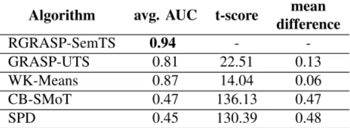
For the hurricane dataset, RGRASP-SemTS had the best average AUC performance achieving 0.94. Compared to the unsupervised algorithms GRASP-UTS and WK-Means, which achieved an average AUC of 0.81 and 0.87 for testing, respectively, the RGRASP-SemTS offers an improvement of at least 0.06in terms of average AUC. The differences in the
TABLE I
COMPARISON OF UNSUPERVISED,SUPERVISED AND SEMI-SUPERVISED ALGORITHMS FOR THE HURRICANES DATASET.
Algorithm avg. AUC t-score mean difference RGRASP-SemTS 0.94 - -GRASP-UTS 0.81 22.51 0.13 WK-Means 0.87 14.04 0.06 CB-SMoT 0.47 136.13 0.47 SPD 0.45 130.39 0.48
mean AUC are significant since the t-score was higher than 2.82, amounting to22.51when compared to GRASP-UTS and 14.04 when compared to the WK-Means. It is important to point out that the WK-Means algorithm received exactly the number of segments that should be found on each trajectory, while the RGRASP-SemTS did not. When compared to the supervised methods named CB-SMoT and SPD, the gains were at least 0.47in terms of avg. AUC.
For the grey seal dataset, RGRASP-SemTS also achieved the best average AUC performance, as depicted in Table II. When RGRASP-SemTS is compared to GRASP-UTS, gains of0.08in were obtained. This difference has significance since the t-score was 14.08 (higher than 2.82). The difference be-tween RGRASP-SemTS and WK-Means were0.07on average AUC in testing. This difference also has a significance, as the t-scorewas6.23. When compared to the supervised methods, namely CB-SMoT and SPD, gains of at least0.37of average AUC were obtained.
TABLE II
COMPARISON OF UNSUPERVISED,SUPERVISED AND SEMI-SUPERVISED ALGORITHMS FOR THE GREY SEALS DATASET.
Algorithm avg. AUC t-score mean difference RGRASP-SemTS 0.88 - -GRASP-UTS 0.80 14.08 0.08 WK-Means 0.81 6.23 0.07 CB-SMoT 0.19 128.69 0.69 SPD 0.53 74.38 0.35 VI. CONCLUSIONS
The research field of trajectory segmentation, although well studied in the literature, has not explored the concept of semi-supervised learning deeply: the use a small set of segments labeled by the user combined with an unsupervised segmentation driven by the training set. The objective is to achieve high accuracy even when few labeled examples are available. This is particularly useful for segmenting trajectories based on semantics.
This paper gives a contribution in this direction since it proposes RGRASP-SemTS, a reactive and semi-supervised algorithm for semantically segmenting trajectory data. This al-gorithm exploits labeled and unlabeled data to find an optimal segmentation of a trajectory by modifying segment landmarks
to achieve homogeneity in the segments using a cost function based on the MDL principle. We performed experiments with two real-world datasets to assess the effectiveness of our approach. The results show that the proposed algorithm outperforms the state-of-art competitors. We intend to extend this work towards several directions. For example we can improve the overall performance by generating better sets of semantic landmarks, instead of just computing averages.
REFERENCES
[1] S. P. A. Alewijnse, K. Buchin, Maike B., A. K¨olzsch, H. Kruckenberg, and M. A. Westenberg. A framework for trajectory segmentation by stable criteria. In22Nd ACM SIGSPATIAL Conference, pages 351–360, New York, NY, USA, 2014. ACM.
[2] V. Bogorny, C. Renso, A. R. de Aquino, F. de Lucca Siqueira, and L. O. Alvares. CONSTAnT a conceptual data model for semantic trajectories of moving objects. Trans. in GIS, 18(1):66–68, 2014. [3] G. A. Breed, I. Jonsen, R. A. M, W. D. Bowen, and M. L.
Leonard. Sex-specific, seasonal foraging tactics of adult grey seals (Halichoerus grypus) revealed by state-space analysis. Ecology, 90(11), 2009.
[4] M. Buchin, A. Driemel, M. Van Kreveld, and V. Sac-ristan. Segmenting trajectories: A framework and algo-rithms using spatiotemporal criteria. Journal of Spatial Information Science, 3(3):33–63, 2011.
[5] P. D. Grunwald, I. J. Myung, and M. Pitt. Advances in Minimum Description Lenght. MIT Press, 2005. [6] M. Hall, E. Frank, G. Holmes, B. Pfahringer, P.
Reute-mann, and I. H. Witten. The weka data mining software: An update.SIGKDD Explor. Newsl., 11(1):10–18, 2009. [7] A. Soares J´unior, B. N. Moreno, V. C. Times, S. Matwin, and L. A. F. Cabral. GRASP-UTS: an algorithm for unsu-pervised trajectory segmentation. Int. J. of Geographical Information Science, 29(1):46–68, 2015.
[8] A. Soares J´unior, C. Renso, and S. Matwin. Analytic: An active learning system for trajectory classification. IEEE Computer Graphics and Applications, 37(5):28– 39, 2017.
[9] Luis A. Leiva and Enrique Vidal. Warped k-means: An algorithm to cluster sequentially-distributed data. Information Sciences, 237(0):196 – 210, 2013.
[10] H. Liu and R. Setiono. Chi2: Feature selection and discretization of numeric attributes. In In Proceedings of the Seventh International Conference on Tools with Artificial Intelligence, pages 388–391, 1995.
[11] J. A. Manso, V. C. Times, G. Oliveira, L. O. Alvares, and V. Bogorny. Db-smot: A direction-based spatio-temporal clustering method. InIEEE International Conference on Intelligent Systems (IS), pages 114–119, 2010.
[12] B. N. Moreno, A. Soares J´unior, V. C. Times, P. Tedesco, and Stan Matwin. Weka-sat: A hierarchical context-based inference engine to enrich trajectories with semantics. In Advances in Artificial Intelligence, pages 333–338, Cham, 2014. Springer International Publishing.
[13] A. T. Palma, V. Bogorny, B. Kuijpers, and L. O. Alvares. A clustering-based approach for discovering interesting places in trajectories. InACMSAC, pages 863–868, 2008. [14] C. Parent, S. Spaccapietra, C. Renso, G. L. An-drienko, N. V. AnAn-drienko, V. Bogorny, M. L. Damiani, A. Gkoulalas-Divanis, J. A. F. de Macˆedo, N. Pelekis, Y. Theodoridis, and Z. Yan. Semantic trajectories mod-eling and analysis. ACM Comput. Surv., 45(4):42, 2013. [15] M. Prais and C. C. Ribeiro. Reactive grasp: An applica-tion to a matrix decomposiapplica-tion problem in TDMA traffic assignment.INFORMS J. on Computing, 12(3):164–176, 2000.
[16] Chiara Renso, Stefano Spaccapietra, and Esteban Zi-manyi, editors. Mobility Data: Modeling, Management, and Understanding. Cambridge Press, 2013.
[17] S. Spaccapietra, C. Parent, M. L. Damiani, J. A. Macedo, F. Porto, and C. Vangenot. A conceptual view on trajectories. DKE, 65(1):126–146, 2008.
[18] Z. Yan, N. Giatrakos, V. Katsikaros, N. Pelekis, and Y. Theodoridis. Setrastream: Semantic-aware trajectory construction over streaming movement data. In12th Int. Conf. on Advances in Spatial and Temporal Databases, SSTD’11, pages 367–385. Springer, 2011.
[19] H. Yoon and C. Shahabi. Robust time-referenced seg-mentation of moving object trajectories. In 2008 Eighth IEEE International Conference on Data Mining, pages 1121–1126. IEEE, December 2008.
[20] Y. Zheng, L. Zhang, Z. Ma, X. Xie, and W. Ma. Rec-ommending friends and locations based on individual location history. ACM Trans. Web, 5(1):5:1–5:44, 2011.