Faculty of Natural Sciences and Technology I
Department of Computer Science
Topics in learning sparse and low-rank models
of non-negative data
Martin Slawski
Dissertation
zur Erlangung des Grades
des Doktors der Naturwissenschaften (Dr. rer. nat.) der Naturwissenschaftlich-Technischen Fakult¨aten der Universit¨at des Saarlandes
Berichterstatter / Reviewers:
Prof. Dr. Matthias Hein
Prof. Dr. Thomas Lengauer, PhD Prof. Jared Tanner, PhD
Pr¨ufungsausschuss / Examination Board:
Prof. Dr. Joachim Weickert Prof. Dr. Matthias Hein
Prof. Dr. Thomas Lengauer, PhD Prof. Jared Tanner, PhD
Dr. Moritz Gerlach
Dekan / Dean:
Prof. Dr. Markus Bl¨aser
Tag des Kolloquiums / Date of the Defense Talk:
February 25th, 2015
Acknowledgments . . . v
Abstract . . . vi
Zusammenfassung. . . vii
Publication record . . . viii
Prologue 1 1 Sparse recovery with non-negativity constraints 4 1.1 Background on sparse recovery and statistical estimation for sparse high-dimensional linear models . . . 8
1.1.1 Problem statement . . . 8
1.1.2 The high-dimensional, sparse setting . . . 9
1.1.3 Practical relevance of the high-dimensional, sparse setting . . . 10
1.1.4 Estimation procedures for sparse high-dimensional linear models 12 1.1.5 Estimation procedures for sparse, non-negative high-dimensional linear models and contributions of this chapter . . . 17
1.2 Preliminaries . . . 19
1.3 Exact recovery and neighbourliness of high-dimensional polyhedral cones 20 1.3.1 Non-negative solutions to underdetermined linear systems of equa-tions and error correcting codes . . . 20
1.3.2 Geometry of polyhedral cones . . . 22
1.3.3 `1/`0 equivalence and neighbourliness of polytopes . . . 27
1.3.4 Construction of sensing matrices. . . 28
1.4 Non-negative least squares (NNLS) for high-dimensional linear models. 34 1.4.1 Prediction error: a bound for ’self-regularizing’ designs . . . 35
1.4.2 Fast rate bound for prediction and bounds on the `q-error for estimation, 1≤q≤2 . . . 40
1.4.3 Asymptotic rate minimaxity . . . 44
1.4.4 Estimation error with respect to the `∞-norm and support re-covery by thresholding . . . 50
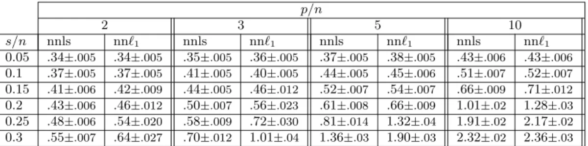
1.4.5 Comparison with the non-negative lasso . . . 60
1.4.7 Proofs of the results on random matrices . . . 76
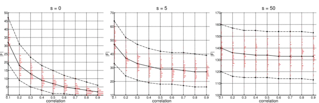
1.4.8 Empirical performance on synthetic data . . . 86
1.4.9 Extensions . . . 93
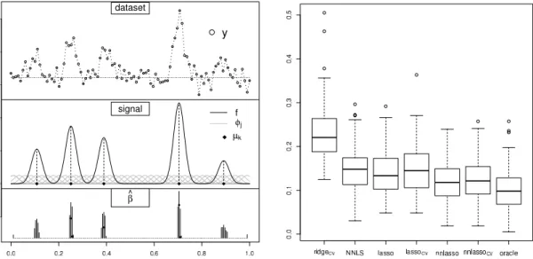
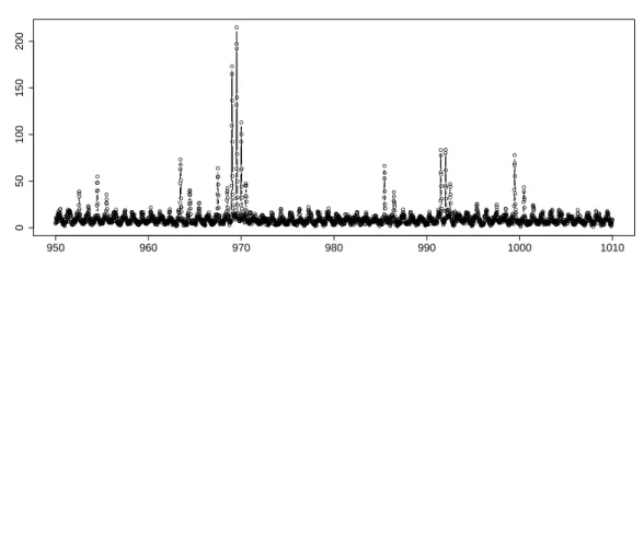
1.5 Sparse recovery for peptide mass spectrometry data . . . 95
1.5.1 Background . . . 96
1.5.2 Challenges in data analysis. . . 96
1.5.3 Formulation as sparse recovery problem . . . 98
1.5.4 Practical implementation . . . 104
1.5.5 Performance in practice . . . 114
2 Matrix Factorization with Binary Components 120 2.1 Low-rank representation and the singular value decomposition . . . 122
2.2 Structured low-rank matrix factorization . . . 123
2.3 Non-negative matrix factorization . . . 124
2.4 Matrix Factorization with Binary Components . . . 126
2.4.1 Applications and related work . . . 127
2.4.2 Contributions . . . 129
2.4.3 Exact case . . . 129
2.4.4 Approach . . . 130
2.4.5 Uniqueness . . . 133
2.4.6 Speeding up the basic algorithm . . . 137
2.4.7 Approximate case . . . 139
2.4.8 Experiments . . . 140
2.4.9 Open problems . . . 146
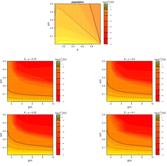
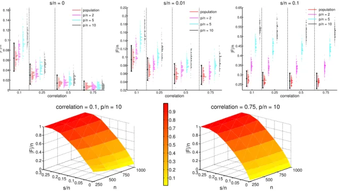
A Addenda Chapter 1 147 A.1 Empirical scaling of τ2(S) for Ens + . . . 147
B Addenda Chapter 2 150 B.1 Example of non-uniqueness under non-negativity of the right factor . . 150
B.2 Optimization for the quadratic penalty-based approach . . . 151
First of all, I would like to thank my thesis advisor Matthias Hein for his guidance. I truly admire his outstanding talent to discover interesting directions of research. All of his suggestions have turned out to be rich and rewarding topics. His quickness of mind, efficiency and precision in his work and his ability to get instantly a good grasp of scientific problems with the help of excellent mathematical intuition, as well as his patience with his students (who may not always be able to think as fast as him) have deeply impressed me throughout the work on this thesis. Matthias’ skills have con-tributed to this thesis in many ways, in particular by helping me out several times when I got stuck. At the same, Matthias gave me plenty of freedom to pursue my own ideas. When preparing my work for publication, he always had very good ideas that would improve my presentation, and he saved me quite a few times by spotting subtle (and also less subtle) flaws in my proofs. Lastly, Matthias let me attend several workshops and conferences which not only gave me the possibility to present my own work, but also to learn from the ideas of other researchers.
Next, I would like to thank Prof. Dr. Lengauer, PhD and Prof. Jared Tanner, PhD for acting as reviewers of this thesis. I am also grateful for the discussion I had with Prof. Tanner during the workshop ’Sparsity and Computation’ at an early stage of the work on this thesis. In fact, this discussion proved to be rather helpful in later stages. During the work of this thesis, I was funded by the cluster of excellence ’Multimodel Computing and Interaction’ (MMCI) of Deutsche Forschungsgemeinschaft. The finan-cial support is gratefully acknowledged.
I thank all persons with whom I collaborated during this thesis: Barbara Gregorius, Andreas Hildebrandt, Rene Hussong, Thomas Jakoby, David James, Janis Kalofolias, Felix Krahmer, Pavlo Lutsik, J¨orn Walter and Qinqing Zheng. Thanks also to Irina Rish and her colleagues for organizing the publication of the book ’Practical Applica-tions of Sparse Modeling’.
I thank all former and present lab members of the machine learning group at Saarland University for a nice working atmosphere.
I also thank my friends for helping me not to ponder about my work all the time. A special thanks goes to Syama Sundar Rangapuram for introducing me to the Indian (especially Telugu-speaking) community in Saarbr¨ucken. Through him, I got to know Srikanth Duddela who has become my best friend here. Without his encouragements, I would probably not have completed this thesis. I will never forgot all the fun we had during table tennis, gym and movie sessions, which helped me to forget about my problems and to stay focused.
This thesis is dedicated to my family. The unconditional support I have experienced throughout my life has been key to my accomplishments.
Advances in information and measurement technology have led to a surge in preva-lence of high-dimensional data. Sparse and low-rank modeling can both be seen as techniques of dimensionality reduction, which is essential for obtaining compact and interpretable representations of such data.
In this thesis, we investigate aspects of sparse and low-rank modeling in conjunction with non-negative data or non-negativity constraints.
The first part is devoted to the problem of learning sparse non-negative representations, with a focus on how non-negativity can be taken advantage of. We work out a detailed analysis of non-negative least squares regression, showing that under certain conditions sparsity-promoting regularization, the approach advocated paradigmatically over the past years, is not required. Our results have implications for problems in signal pro-cessing such as compressed sensing and spike train deconvolution.
In the second part, we consider the problem of factorizing a given matrix into two factors of low rank, out of which one is binary. We devise a provably correct algorithm computing such factorization whose running time is exponential only in the rank of the factorization, but linear in the dimensions of the input matrix. Our approach is extended to noisy settings and applied to an unmixing problem in DNA methylation array analysis. On the theoretical side, we relate the uniqueness of the factorization to Littlewood-Offord theory in combinatorics.
Fortschritte in Informations- und Messtechnologie f¨uhren zu erh¨ohtem Vorkommen hochdimensionaler Daten. Modellierungsans¨atze basierend auf Sparsity oder niedrigem Rang k¨onnen als Dimensionsreduktion betrachtet werden, die notwendig ist, um kom-pakte und interpretierbare Darstellungen solcher Daten zu erhalten.
In dieser Arbeit untersuchen wir Aspekte dieser Ans¨atze in Verbindung mit nichtneg-ativen Daten oder Nichtnegativit¨atsbeschr¨ankungen.
Der erste Teil handelt vom Lernen nichtnegativer sparsamer Darstellungen, mit einem Schwerpunkt darauf, wie Nichtnegativit¨at ausgenutzt werden kann. Wir analysieren nichtnegative kleinste Quadrate im Detail und zeigen, dass unter gewissen Bedingungen Sparsity-f¨ordernde Regularisierung - der in den letzten Jahren paradigmatisch enpfoh-lene Ansatz - nicht notwendig ist. Unsere Resultate haben Auswirkungen auf Probleme in der Signalverarbeitung wie Compressed Sensing und die Entfaltung von Pulsfolgen. Im zweiten Teil betrachten wir das Problem, eine Matrix in zwei Faktoren mit niedrigem Rang, von denen einer bin¨ar ist, zu zerlegen. Wir entwickeln daf¨ur einen Algorith-mus, dessen Laufzeit nur exponentiell in dem Rang der Faktorisierung, aber linear in den Dimensionen der gegebenen Matrix ist. Wir erweitern unseren Ansatz f¨ur ver-rauschte Szenarien und wenden ihn zur Analyse von DNA-Methylierungsdaten an. Auf theoretischer Ebene setzen wir die Eindeutigkeit der Faktorisierung in Beziehung zur Littlewood-Offord-Theorie aus der Kombinatorik.
Many parts of this thesis have been published before. We here provide an overview on the underlying publications.
§1.3, 1.4 are to great parts based on:
M. Slawski and M. Hein.
Non-negative least squares for high-dimensional linear models: consistency and sparse recovery without regularization.
The Electronic Journal of Statistics, 7:3004–3056, 2013.
M. Slawski and M. Hein.
Sparse recovery by thresholded non-negative least squares.
Advances in Neural Information Processing Systems, 24:1926–1934. 2011.
M. Slawski and M. Hein.
Robust sparse recovery with non-negativity constraints.
4th Workshop on Signal Processing with Adaptive Sparse Structured Representations (SPARS), p.30, 2011.
§1.5 is based on:
M. Slawski, R. Hussong, A. Tholey, T. Jakoby, B. Gregorius, A. Hildebrandt, and M. Hein.
Peak pattern deconvolution for protein mass spectrometry by non-negative least squares/least absolute deviation template matching.
BMC Bioinformatics, 13:291, 2012.
M. Slawski and M. Hein.
Practical Applications of Sparse Modeling, edited by I. Rish, G. Cecchi, A. Lozano and A. Niculecu-Mizil, chapter ’Sparse Recovery for Protein Mass Spectrometry Data’. MIT press. In press.
§2 is based on:
M. Slawski, M. Hein, and P. Lutsik.
Matrix Factorization with Binary Components.
During and before the work on this thesis, the author published several additional papers whose results are not presented here.
M. Slawski and M. Hein.
Positive definiteM-matrices and structure learning in attractive Gaussian Markov ran-dom fields.
Linear Algebra and its applications. In press.
M. Slawski
The structured elastic net for quantile regression and support vector classification.
Statistics and Computing, 22, 153-168, 2012.
M. Slawski, W. zu Castell, and G. Tutz
Feature Selection Guided by Structural Information.
Annals of Applied Statistics, 4, 1056-1080, 2010.
A.-L. Boulesteix and M. Slawski
Stability and Aggregation of ranked gene lists.
Briefings in Bioinformatics, 10, 556-568, 2009.
M. Slawski, M. Daumer, and A.-L. Boulesteix
CMA - a comprehensive Bioconductor package for supervised classification with high-dimensional data
We have reached an era in which it is easy to collect, store, access and disseminate large data sets. While the information contained therein may carry a lot of potential for science, engineering and business, the analysis of such data poses new challenges such as massive sample size or high dimensionality. The latter refers to the availability of many attributes (’variables’) per datum which can be critical, among others, for the following reasons.
Lack of interpretability: the results of data analysis tend to be difficult to interpret unless they involve a suitable condensed representation of the given data.
Reduced statistical performance: it is well documented in existing literature that sev-eral traditional data analysis techniques routinely used in a low-dimensional setting exhibit poor statistical performance when applied to data sets for which the ratio of the sample size and the number of variables is small. This situation bears the danger of overfitting, or more generally, noise accumulation ([60], §3.2).
High computing times: it is clear that performing standard tasks such as regression, classification or clustering consumes more time the more variables are taken into ac-count. In some applications their number can be in the order of millions so that e.g. prediction of future observations may become impractically slow.
These issues indicate that it is worthwhile to consider some form of (linear) dimen-sion reduction as an integral part of data analysis. In fact, high-dimendimen-sional data sets usually possess low-dimensional structure to be exploited. Sparsity and low-rank struc-ture are among the best studied examples over the past few years. Here, sparsity refers to the situation where a given task can be tackled by identifying a comparatively small subset of relevant variables, while low-rank structure refers to a data matrix which is (effectively) of low rank, or in geometrical terms, to data points residing approxi-mately in a low-dimensional linear subspace. In this thesis, we investigate aspects of both concepts in the presence of non-negative data or non-negativity constraints. A major portion is devoted to the analysis of non-negative least squares, an optimization problem one encounters when fitting linear models with non-negative parameters of the form
y≈X1β1∗+. . .+Xpβp∗, β
∗
j ≥0, j = 1, . . . , p, (0.1)
where y = (yi)ni=1 represents a set of observations linked to given explanatory or
pre-dictor variables Xj, j = 1, . . . , p. The standard method for inferring the parameters {βj∗}pj=1 is by minimizing the least squares criterion
min
{βj}pj=1
In case the parameters are known to be non-negative, it is recommended to impose corresponding constraints. For example, model (0.1) is suited to situations where the observations arise from an addition of certain components whose abundances are quantified in terms of the {βj∗}pj=1. The setting in whichboth the parameters and the explanatory variables are non-negative is studied in greater depth in this thesis. Our specific interest is motivated by the fact that a good deal of contemporary data such as binary (0/1) data, counts or intensities (e.g. greyscale images) have a non-negative range. A distinctive feature of the two-fold non-negativity is that terms in the sum in (0.1) can no longer cancel out. This property bears the potential to curb overfitting. It also turns out to have a remarkably positive effect under sparse scenarios in which most of the {βj∗}pj=1 are zero or of negligible magnitude. More specifically, the explicit promotion of sparsity by means of a data-independent regularization term as made popular by methods like the lasso [36, 151], may no longer be required. This opens up a conceptually much simpler approach to sparse recovery, i.e. identification of the set of relevant predictor variables {j : βj∗ 6= 0}.
The power of non-negativity was recognized earlier, but solid theoretical evidence for empirical observations has been scarce − a gap that we try to bridge in this the-sis. Our findings also shed some light on non-negative matrix factorization (NMF), a popular method of linear dimension reduction for non-negative data. Given a set of non-negative data points dj ∈ Rm+, j = 1, . . . , n, NMF aims at finding a set of points
tk ∈ Rm+, k = 1, . . . , r, with r <min{m, n} chosen according to the desired dimension
reduction such that
dj ≈t1α1j +. . .+trαrj (0.2)
for non-negative coefficients αkj, j = 1, . . . , n, k = 1, . . . , r. Note that for each j,
(0.2) constitutes a linear model of the form (0.1), with the important difference that there are no fixed predictor variables; the {tk}rk=1 and the coefficients{αkj}need to be
inferred simultaneously. This can be recast as the optimization problem
min T∈Rm+×r, A∈R r×n + kD−T Ak2 F = min T∈Rm+×r, A∈R r×n + m X i=1 n X j=1 (Dij−(T A)ij)2, (0.3)
where the columns of the matricesDandT contain the{dj}jn=1respectively the{tk}rk=1 and A = (αkj). In their seminal paper [92], Lee and Seung argue that NMF has
tendency to yield a parts-based decomposition of the data matrix D in which the ’parts’ {tk}rk=1 and the associated coefficients are sparse. This phenomenon can be better understood in light of our analysis of non-negative least squares under two-fold non-negativity. In fact, problem (0.3) collapses into n independent non-negative least squares problems of the form
min
{αkj≥0}rk=1
kdj−t1α1j −. . .−trαrjk22, j = 1, . . . , n,
once the matrix T is known (and vice versa if A is known). This observation also un-derlies the common alternating updates approach to optimize the NMF criterion (0.3). However, such scheme cannot be shown to yield a global minimizer. Indeed, solving (0.3) globally optimally yields a computational challenge in general. Specifically, even in the exact case in which it holds that D = T A with T and A non-negative, finding
such factorization has been shown to be NP-hard in [160]. The influential paper by Arora et al. [3] has given fresh impetus to the field. In that paper, the authors show that the exact NMF problem can be solved by linear programming under a certain condition fulfilled in several important applications of NMF.
In the second chapter of this thesis, we discuss the computation of a special case of NMF in which one of the two factors is required to be binary. We show that in a wide range of cases, solving NMF problems with one binary factor remains computationally tractable as long as the inner dimension r of the factorization remains small. This may come as a surprise since− at least at first glance − the additional combinatorial constraints seem to add another layer complexity to an already challenging problem. In summary, we hope to convey the idea that non-negativity is a common yet pow-erful constraint that can be of enormous use in data analysis, and that offers various interesting directions of research.
Sparse recovery with non-negativity constraints
The problem of learning sparse representations from few samples has received enormous attention in the past ten to fifteen years in a variety of disciplines in mathematics, engineering, and computer science. Interest in this problem has evolved from the practical need to find compact representations of high-dimensional objects (e.g. images or videos), in order to enable efficient compression and sampling [18, 144], as well as from the search for statistically sound methods dealing with high-dimensional feature spaces [19, 82]. In this work, we study sparse, non-negative representations, with a specific focus on how the additional sign constraint can be harnessed in terms of statistical theory and practical data analysis.
Chapter outline. We start by providing an overview on high-dimensional linear mod-els and sparse estimation, the theme of this chapter. It consists of a theoretical and a practical part. The theoretical part follows a division into a noiseless and a noisy setup. For the former, we consider the problem of recovering a sparse non-negative vector from underdetermined linear systems of equations and discuss the underlying geometry. Our treatment of the noisy setup focuses on a detailed analysis of non-negative least squares within a modern framework of high-dimensional statistical inference. The practical part is devoted to an in-depth case study in proteomics, which is used to highlight the usefulness of non-negative least squares in applications. A list of contributions of this chapter can be found in §1.1.5.
Notation table for this chapter.
:= equality by definition; we use plain ’=’ if context is clear
I(·) indicator function vI subvector of v ∈Rm corresponding to I ⊆ {1, . . . , m} kvkq `q-(quasi)-norm of v ∈Rm, i.e. kvkq = ( Pm i=1v q i) 1/q
for q∈(0,∞) and kvk∞= max1≤i≤m|vi|
kvk0 `0-’norm’ ofv, i.e. kvk0 =Pmi=1I(vi 6= 0)
Sc complement of S (if ground set is clear from the context)
|S| cardinality of a set S
B0(S;p) vectors in Rp with support included in S ⊆ {1, . . . , p},
i.e. B0(S;p) = {v ∈Rp : v
j = 0 ∀j /∈S}
B0(s;p) vectors in Rp with at most s non-zero entries, i.e.
B0(s;p) = {v ∈Rp : kvk
0 ≤s}
R+ non-negative real line, i.e. R+ ={x∈R: x≥0}
B0+(S;p) B0(S;p)∩Rp+
B0+(s;p) B0(s;p)∩Rp+
J(k), sets of all subsets of {1, . . . , p}of cardinality k, i.e.
0≤k ≤p J(k) = {J ⊆ {1, . . . , p}: |J|=k}
hv, wi usual inner product of v, w∈Rm, i.e. hv, wi=Pm
i=1viwi
v w vi ≥wi, i= 1, . . . , m. Analogous for , ,≺.
x∨y,x∧y max{x, y}, min{x, y}
bxc largest integer less than or equal to x
Tm−1 probability simplex in
Rm+, i.e. Tm ={x∈Rm+ :
Pm
i=1xi = 1}
intA interior of some set A⊆Rm (w.r.t. the usual topology)
bdA boundary of some set A⊆Rm (w.r.t. the usual topology)
MIJ submatrix of a real m×n matrix M corresponding to rows in I ⊆ {1, . . . , m}and columns in J ⊆ {1, . . . , n}
MJ submatrix ofM corresponding to columns in J;M∅ := 0
Mj j-th column of M
Mj (transpose of the) j-th row of M
[M, M0] column-wise concatenation of matrices M, M0
[M; M0] row-wise concatenation of matrices M, M0
N(M) nullspace of a real matrixM, i.e.
N(M) ={x∈Rn :M x= 0}
tr(M) trace of a square matrix M, i.e. tr(M) =Pm
i=1Mii
CM conic hull of the columns of M, i.e.
CM ={y∈Rm : y=M λ, λ∈Rn+}
PM convex hull of the columns of M, i.e.
PM ={y∈Rm : y=M λ, λ∈Rn+,
Pn
i=1λi = 1} P0,M convex hull of the columns of M and the origin, i.e.
P0,M ={y∈Rm : y=M λ, λ∈Rn+,
Pn
i=1λi ≤1}
Im identity matrix of dimension m,
I identity matrix of unspecified dimension (context)
{ei}mi=1 canonical basis vectors of Rm
1, 1 vector respectively matrix of ones
E[Z] expectation of some random variable Z
Var[Z] variance of some random variable Z
P(A) probability of some event A
Z ∼N(µ, C) random vector Z follows a Gaussian distribution with mean µand covariance C
Y =D Z the random variablesY and Z follow the same distribution
f(x) =o(g(x)) lim x→a|f(x)/g(x)|= 0 as x→a f(x) =O(g(x)) lim sup x→a |f(x)/g(x)|<∞ as x→a f(x) = Ω(g(x)) lim inf x→a |f(x)/g(x)|>0 as x→a f(x) = Θ(g(x)) 0<lim inf x→a |f(x)/g(x)| ≤lim supx→a |f(x)/g(x)|<∞ as x→a
Xn=oP(g(n)) Sequence of random variables {Xn} satisfies
∀ε >0 limn→∞P(|Xn/g(n)| ≥ε) = 0.
Xn=OP(g(n)) Sequence of random variables {Xn} satisfies
∀δ >0 ∃c <∞ such that P(|Xn/g(n)| ≥c)< δ ∀n.
c, c0, c1, C, C0, C1 etc. positive constants (value may differ from line to line)
Abbreviations, acronyms, and terminology
i.i.d. independent identically distributed (l/r).h.s. (left/right) hand side
MSE mean squared error
NNLS non-negative least squares PSF point spread function s.t. such that
sb. to subject to w.r.t. with respect to
1.1. Background on sparse recovery and statistical estimation for sparse high-dimensional linear models
In this section, we give a general overview on the topic under consideration and discuss its relations to several areas of recent research.
1.1.1 Problem statement
For what follows, we consider observations y ∈ Rn, which are modelled according to
the linear model
y=Xβ∗+ε, (1.1)
where the right hand side is composed of the following quantities.
• X ∈Rn×p is referred to as design matrix. Depending on the context, X may be
regarded as fixed (fixed design) or random (random design).
• β∗ ∈ Rp+ is a non-negative vector with support S = {j : βj∗ > 0}. We write
s=|S| for its cardinality, to which we refer as sparsity level.
• ε represents an error term whose components (εi)n
i=1 are typically i.i.d. random (’noise’) variables. If ε = 0, we speak of the noiseless case and otherwise of the
noisy case.
The goal is to infer the unknown parameter β∗ given (X, y), i.e. one wants to find an estimator θb=θb(X, y) that estimates accurately the target β∗ contained in the
param-eter set B0+(s;p) = {β ∈Rp+ : kβk0 ≤s} with respect to one of the following criteria.
Exact recovery. In the noiseless case, one mostly aims at having θb=β∗.
Estimation error. In the noisy case, exact recovery is not possible in general. A natural measure for the goodness of approximation is the error in `q-norm kbθ−β∗kq
for some q∈[1,∞].
Prediction error. In the noisy case, one may be interested in reducing the contam-ination of the observations by the noise ε(denoising). A common measure is the mean squared (prediction) error (MSE) 1
nkXθb−Xβ
∗k2
2. The term ’prediction error’ here stems from the fact that for deterministicX, this quantity reveals how well on average
Xθbpredicts a new set of observations ey=Xβ∗+εeif eε is a zero-mean random vector
independent of ε: E 1 nkye−Xθbk 2 2 y =E 1 nkXβ ∗− Xθb+ e εk2 2 y = 1 nkXθb−Xβ ∗k2 2+E 1 nkeεk 2 2 = 1 nkXβ ∗− Xθbk22+ const.,
because the second term does not depend on θb. For the second identity, we have
invoked the assumption that E[εe] = 0. As discussed in subsequent sections, the MSE is a suitable criterion if it is not possible to derive a reasonable upper bound on the estimation error due to high correlations among subsets of columns ofX. On the other hand, an upper bound on the`2-estimation error trivially yields a bound on the MSE:
1 nkXθb−Xβ ∗k2 2 ≤φmax 1 nX > X kθb−β∗k22,
whereφmax(M) denotes the largest eigenvalue of a real symmetric matrix M.
Support recovery or sign consistency. In a sparse regime in which the sparsity level of
β∗ is substantially smaller than the dimension, it is desirable to have a sparse estimator
b
θ whose support {j : θbj = 06 } agrees with that of β∗ (i.e. θbrecovers the support of
β∗), because it means that one has achieved a correct reduction in model complexity. This aspect roots in the problem of variable or feature selection in linear regression [113]. Sign-consistency is a slightly more stringent notion than support recovery, which requires that sign(θbj) = sign(βj∗), j = 1, . . . , p. Clearly, if the estimator θbtakes values
inRp+, the two notions coincide.
1.1.2 The high-dimensional, sparse setting
In the present work, we focus on the ’high-dimensional, (but) sparse regime’ of modern statistical theory ([19],§1), which is outlined in the sequel. Classical statistical estima-tion theory studies the behaviour of an estimator for a fixed parameter set while the sample sizen tends to infinity. This framework has lost in importance because it does not cover several other regimes relevant to modern data analysis. As to our problem introduced above, consider the least squares estimator
b βols ∈argmin β∈Rp 1 nky−Xβk 2 2. (1.2)
Suppose thatX is deterministic and, for simplicity, thatεhas i.i.d. zero-mean Gaussian entries. Let ΠX denote the projection on the column space of X of dimension d =
tr(ΠX). From Xβbols = ΠXy =Xβ∗+ ΠXε, we obtain the following for the prediction
error ofβbols 1 nkXβb ols−Xβ∗k2 2 = 1 nkΠXεk 2 2 =OP(d/n) =OP(p/n). (1.3) We may draw the conclusion that the prediction error of βbols vanishes asymptotically
asn → ∞whilepstays fixed. On the other hand, such asymptotic consideration is not meaningful from a practical point of view if the given data (X, y) do not well reflect this scenario because p is actually similarly large as n or even larger. The fact that the prevalence of such data has dramatically increased in recent years (cf. the following subsection), together with considerable advance in theory, has led to a novel framework whose innovations are summarized below.
Increasing sequence of parameter sets. The parameter set is allowed to increase with
n. For the problem under consideration with parameter set B0+(s;p) this means that the problem dimensionp=pn, the sparsity level s=sn and thusβ∗ =βn∗ may depend
on n. Accordingly, asymptotics are understood with respect to a a triangular array of observations {(X(n), y(n)), X(n) ∈
Rn×pn}, n = 1,2, . . . For notational simplicity,
dependence on n is usually suppressed. Therefore, we here stress that any quantity depending on n via p,s orβ∗ can, in general, no longer be regarded as a constant.
Non-asymptotic analysis. A non-asymptotic analysis, in which results are stated for finite sample sizes, is preferred, even though one typically thinks ofnbeing large when interpreting these results.
Leveraging sparsity. In order to establish reasonable performance guarantees even
if p > n, one needs to assume that the problem is sufficiently sparse, i.e. that s is
small relative to n. In this case, the set B0(s;p) = {β ∈Rp : kβk
0 ≤s}, which is the union of all subspaces spanned by selections of s canonical basis vectors, is effectively a low-dimensional object. Moreover, one needs to work with estimators that are able take advantage of such structure.
We remark that the assumption of exact sparsity, i.e. sparsity in an `0-sense, can be relaxed to various forms of approximate sparsity, in which β∗ is not required to have few non-zero entries but instead few entries of significant magnitude. Common models of approximate sparsity can be found in [124], §2.1. We restrict ourselves to exact sparsity, apart from a single theorem (Theorem 1.28).
Scalings of p and s: regimes of interest. We now discuss specific scalings ofpand s
with n that have been frequently considered in the literature and which are of interest in this work. When speaking of a ’high-dimensional setting’, we suppose that we have at least p = Θ(n) up to p = o(exp(nξ)) for some 0 < ξ < 1. Note that for p = o(n),
even ordinary least squares tends to perform well (cf. (1.3)), hence this regime is not of specific interest. In the noiseless case, we restrict our attention to the situationn < p. Regarding the scaling of s, the regimep= Θ(n) = Θ(s), s < n < p, which is typically referred to as regime of linear sparsity [163] or proportional growth setting [51], is of particular interest in the noiseless case. In the noisy case, it is standard to assume sublinear sparsity in the sense that s=o(n/logp).
1.1.3 Practical relevance of the high-dimensional, sparse setting
The high-dimensional, but sparse setting is not only a construct for theoretical analysis. In fact, such setting is ubiquitous in contemporary applications, a selection of which is outlined below.
Learning from many features. The linear model (1.1) arises in linear regression, where the goal is to model an outcome variable as a linear combination of (input) variables,
predictors or features. The high-dimensional setting has gained in importance in this context, among others, for the following reasons.
• Since the advent of the digital age and the associated advances in information technology, it is cheap to collect and store many attributes per observation. The hope is that the more information, i.e. the more attributes, are taken into account, the more accurately an outcome variable of interest can be predicted.
• It is common to augment the set of given features by additionally considering nonlinear transformations thereof, e.g. powers, logarithm, or products of several features (see pp.139-141 in [74] for more examples). The thus ’enriched’ feature set is supposed to yield more flexibility in modelling and in turn also improved performance in prediction. At the same time, the number of featurespmay grow quickly depending on the transformations considered. For example, if p denotes the original number of features and one considers all products involving up to d
features, we end up with p >(p/d)d features.
• In data from high-throughput biological experiments, for example gene expression microarrays, it is common to have few observations but many features (n p
set-up). We refer to [10] for an overview.
Sparsity, on the other hand, is a reasonable assumption as long as only a small fraction of all predictors considered have a significant effect on the outcome variable. Moreover, sparse models are desired from the points of view of interpretation and computation (e.g. in order to reduce time and storage requirements for prediction).
Sparse approximation with overcomplete systems. This topic has received much at-tention in mathematical signal processing (see e.g. [18], §4.2 and §4.3) and concerns the sparse representation of a given signal y ∈ Rn in a union of bases of
Rn. This
model is suitable whenever the signal arises from a superposition of heterogeneous components.
Inverse problems. The matrix X may also represent operations that lead to a de-graded versionyof some underlying signalβ∗. For exampleymay be a blurred version of some image β∗. Within this thesis, specific attention is paid to sparse spike train deconvolution, where the locations of the non-zero entries in β∗ indicate the positions of spikes andX represents convolution of the spike train with a point-spread function (PSF)and possible down-sampling (cf.§1.5). Typically, problems of this kind fall into the regimep= Θ(n).
Compressed sensing. Compressed sensing (CS) is a modern sampling paradigm in
signal processing pioneered in [31, 33, 45] from which an entire new field of research has emerged, see [56, 124] for an overview. The goal of CS is to recover a signal
β∗ ∈ Θ ⊆ Rp from few samples (one often speaks of measurements in this context),
where the process of sampling or at least aspects thereof can be designed by the user. CS consists of two basic steps termed sampling and decoding. In the sampling step, one obtains measurements yi = gi(β∗;{yu}u≤i), i = 1, . . . , n, n p, for functions gi : Θ→Rthat may depend on all preceding measurements {yu}u≤i,i= 1, . . . , n. The
decoding step consists of a mapping ∆ :Rn→Θ whose goal is to recover β∗ from the
measurements y. While in general the measurement process may be both non-linear (i.e. the functions{gi}ni=1 may be non-linear inβ∗) and adaptive (the functions{gi}ni=1
may be chosen depending on earlier measurements), it is the case of linear and non-adaptive measurements with yi = hXi, β∗i, Xi ∈ Rp, i = 1, . . . , n that has received
most attention in the literature. Note that this case is subsumed by our linear model (1.1) with the {Xi}n
i=1 stacked into the rows of the matrixX (the error termε can be used to model noise in the measurement process), and the decoding step of CS becomes a special case of the problem under consideration. A crucial difference from the setups in regression or deconvolution discussed above is that in CS, the matrix X is regarded as an object that may be chosen freely from the set ofn×preal matrices. In particular, various random constructions of X were considered already at early stages of CS.
1.1.4 Estimation procedures for sparse high-dimensional linear models
Before discussing the peculiarities of the sparse, non-negative case with β∗ ∈B0+(s;p), which is in the center of this thesis, we first provide a short survey on the sparse case with β∗ ∈ B0(s;p). If s is known, a straightforward approach directly incorporating the given prior knowledge about the target is `0-constrained least squares estimation which yields the estimator
b β`0,s ∈ argmin β∈B0(s;p) 1 nky−Xβk 2 2. (1.4)
Under the condition φmin(2s)>0, where for k ∈ {1, . . . , p}
φmin(k) = min δ∈B0(k;p)\{0} kXδk2 2 nkδk2 2 , (1.5)
the following statement establishes several performance guarantees forβb`0,s. Our proof
closely follows the proof of Theorem 2 in [123].
Proposition 1.1. Consider the linear model (1.1) with β∗ ∈ B0(s;p) and support
S ={j : βj∗ 6= 0}. Suppose that φmin(2s)>0 and denote A = max1≤j≤p|Xj>ε|/n. We then have kβb`0,s−β∗kqq ≤ 2q+1Aqs {φmin(2s)}q, q ∈[1,2], and 1 nkXβb `0,s−Xβ∗k2 2 ≤ 8A2s φmin(2s). (1.6) Furthermore, if minj∈S|βj∗| > (2A√2s)
{φmin(2s)}, it holds that sign(βb `0,s
j ) = sign(β
∗
j), j =
1, . . . , p.
Proof. From the definition of βb`0,s, we get
1 nky−Xβb `0,sk2 2 ≤ 1 nky−Xβ ∗k2 2. Let δ=βb`0,s−β∗. Using that y=Xβ∗+ε, it follows that
1 nkXδk 2 2 ≤ 2 n δ, X>ε≤2Akδk1, (1.7)
where the second inequality results from H¨older’s inequality and the definition of A. Noting that δ∈B0(2s;p), we obtain according to the definition of φmin(2s)
φmin(2s)kδk2 2 ≤ 1 nkXδk 2 2 ≤2Akδk1
The fact thatδ ∈B0(2s;p) also implies thatkδk2
2 ≥ kδk21/2s and thus kβb`0,s−β∗k1 =kδk1 ≤ 4A s φmin(2s), and kβb `0,s−β∗k2 2 =kδk 2 2 ≤ 8A2s {φmin(2s)}2 (1.8)
Substituting the bound on kδk1 back into (1.7), we obtain the second part of (1.6). The general`q-bound results from the inequality kδkqq ≤ kδk
2q−1 1 kδk
2(q−1)
2 , which holds for all q∈[1,2]. As to the second part of the statement, we have from (1.8)
2A√2s φmin(2s) ≥ kβb `0,s−β∗k 2 ≥ kβb`0,s −β∗k∞ ≥max j∈S | b β`0,s j −β ∗ j|
If there were a j ∈S such that sign(βbj`0,s)= sign(6 βj∗), the lower bound on minj∈S|βj∗|
would lead to a contradiction. Consequently, we must have sign(βbj`0,s) = sign(βj∗),
j ∈S and in turn kβb`0,sk0 =s and hence also βbj`0,s = 0 for allj ∈Sc.
Proposition1.1 reveals that from a mere statistical point of view, `0-constrained least squares allows one to cope with the high-dimensional, sparse setting. All bounds depend on ponly via φmin(2s) (it turns out not to be restrictive to assume the scaling
φmin(2s) = Ω(1)) and the term A that represents the influence of the error term. Specializing to ε = 0, Proposition 1.1 asserts exact recovery, i.e. βb`0,s = β∗. If ε has
i.i.d. zero-mean Gaussian entries and max1≤j≤pkXjk = O( √
n), one can show that
A=OP(log(p)/n) (cf. the proof of Theorem 1.21 below). The bounds (1.6) then yield
kβb`0,s−β∗k22 =OP(slog(p)/n), and
1
nkXβb
`0,s−Xβ∗k2
2 =OP(slog(p)/n). (1.9) The bound on the prediction error constitutes a drastic improvement over the corre-sponding bound for least squares estimation (1.3). In contrast to the latter, the bound for βb`0,s reflects the sparsity of the problem with linear dependence on s in place of
p, which now enters only logarithmically. Apart from the extra log factor, the bounds (1.9) match the performance of an estimator one would use if one had access to an oracle revealing the support of β∗:
b βoracle ∈ argmin β∈Rp:βSc=0 1 nky−Xβk 2 2. (1.10)
The second part of Proposition 1.1 implies that if all non-zero entries of β∗ are suffi-ciently large, then βb`0,s = βboracle. However, in practice it is basically as unrealistic to
• `0-constrained least squares estimation is a non-adaptive estimation procedure in the sense that the sparsity level of the problem needs to be known in advance in order to achieve performance bounds of the correct order. In contrast, an adaptive estimation procedure achieves optimal performance simultaneously over a broad range of sparsity levels. In [23] it is shown that under assumption of i.i.d. zero-mean Gaussian errors ε, adaptivity is achieved when using `0-penalized
orregularized least squares estimation
b β`0,λ ∈argmin β∈Rp 1 nky−Xβk 2 2+λkβk0, λ >0, (1.11)
with proper choice of the regularization parameter λ. Unfortunately, such choice depends on the variance of the error terms, which is typically not known in practice.
• Even in case sor a suitable value ofλ were known, it would still not be practical to work with (1.4) respectively (1.11) for computational reasons. Computingβb`0,s
in the most obvious way involves checking all Ps
k=0
p k
subsets of {1, . . . , p} of cardinality less than or equal to s, which is not feasible in practice unless s is tiny (say s ≤ 3) or p is small (state-of-the-art branch-and-bound methods [76] may handle cases with p up to 50). From the point of view of computational complexity, several hardness results have been established [2, 114]. There do exist algorithms that can be shown to deliver βb`0,s under certain conditions on
the data (X, y) (see the subsequent paragraph for examples). However, verifying these conditions is in turn NP-hard or conjectured to be NP-hard [152].
Overall, the discussion of `0-constrained estimation has touched upon crucial criteria based on which different estimation procedures should be compared.
• What performance guarantees regarding prediction, estimation and support re-covery can be established ?
• What conditions on X and minj∈S|βj∗| are required to achieve these guarantees,
and are these conditions likely to be fulfilled for a given problem ?
• What is the computational effort needed to compute the estimator ?
• What is the degree of adaptivity of the procedure, i.e. which tuning parameters need to be specified and can these tuning parameters be chosen in a data-driven manner without explicit knowledge of problem-specific quantities ?
In the sequel, we discuss a selection of estimation procedures proposed in the literature in light of the considerations above.
Practical approaches to (approximate) `0-constrained or regularized estimation. In the preceding discussion, we have thought of (1.4) and (1.11) as obtaining the glob-ally optimal solution to a combinatorial optimization problem. A different approach is to treat (1.4) as an instance of nonlinear programming and then apply an algorithm
from this field that allows one to circumvent the combinatorial nature of the problem. The use of gradient projection is most prominent in this context [14], as it can be exploited that it is trivial to compute the Euclidean projection onB0(s;p). This yields a practical scheme, for which performance guarantees can be established if X satis-fies certain forms of the restricted isometry property originally introduced in [30, 31]. Roughly speaking, this condition requires that 1
nX
>X nearly acts as an isometry on
B0(2s;p), which is much more restrictive than the conditionφmin(2s)>0, cf. (1.5). An alternative approach [150] applicable to both (1.4) and (1.11) is a reformulation within a certain class of optimization problems known as DC programs [42]. No performance guarantees appear to have been established for the approach in [150] so far.
Another line of research concerned with (1.11) considers families of functions that are smooth (apart from single points) and that can approximate the functionx7→I(x6= 0) arbitrarily well. A classical example is the family of `q-quasinorms with x 7→ |x|q, q ∈(0,1), see [64] and [174] for more examples. The resulting optimization problems are non-convex, which considerably complicates theoretical analysis due to the presence of multiple local optima, see [164,174].
Convex relaxation: `1-regularization. The probably most popular approach to sparse high-dimensional regression is`1-regularized least squares estimation
b β`1,λ ∈argmin β∈Rp 1 nky−Xβk 2 2+λkβk1, λ >0, (1.12)
which results from (1.11) by replacing the`0-’norm’ by its convex envelope1 on [−1,1]p.
This motivates the use of term convex relaxation here. Convexity entails that a globally optimal solution of (1.12) can be found using one out of a whole battery of efficient algorithms [137]. `1-regularized least squares estimation has a long history in statistics [151] under the acronym ’lasso’ (which will also be used here) as well as in signal processing [36]. The ’Dantzig selector’ [32] is a highly similar approach. In the noiseless case, both these approaches amount to `1-minimization
b
β`1 ∈argmin β∈Rp
kβk1 sb. to Xβ =y, (1.13)
which coincides with (1.12) in the limit λ → 0 provided (1.13) is feasible. By now, there is a substantial body of work [30, 31, 39, 43, 44,46, 47, 51, 61, 132,178] on the question of `1/`0-equivalence in the noiseless case, where `1-minimization is related to
`0-minimization
b
β`0 ∈argmin β∈Rp
kβk0 sb. to Xβ =y. (1.14)
One speaks of `1/`0-equivalence if the solutions of both (1.13) and (1.14) are unique and agree, in which case `1-minimization achieves exact recovery. One of the major findings is that for certain classes of random matrices`1/`0-equivalence holds for a wide range of scalings of the triple (n, p, s) (cf. end of §1.1.2), which underlies a remarkable high-dimensional geometric phenomenon [43,46,51] to be discussed in more detail for the non-negative case in §1.3.3 below.
1The convex envelope of a function is its tightest convex underapproximate. More precisely, it is its biconjugate [129],§12.
In the noisy case, the lasso (1.12) and `0-regularization (1.11) can no longer be exactly equivalent, but they tend to have comparable performance with regard to estimation in `q-norm, q ∈ [1,2], and prediction error (cf. Proposition 1.1), under the conditions
that, roughly speaking, the design X would satisfy `1/`0-equivalence in the noiseless case, and the regularization parameter λ is properly specified [11, 58, 110, 122, 123, 156, 157, 173, 182]. On the other hand, the situation is noticeably different from the noiseless case in the sense that the lasso does not achieve sign consistency/support recovery irrespectively of howλ is chosen, unlessX satisfies a specific condition, which is rather restrictive [95,109,163,180,184]. This failure occurs irrespective of how large minj∈S|βj∗| is and can be traced back to the bias of the `1-regularizer that shrinks all
components of βb`1,λ towards zero, including those corresponding to the support ofβ∗,
where such shrinkage is actually not desired. The lasso tries to compensate for that shrinkage by including extra predictors corresponding toScso that
b
β`1,λ
Sc tends to have
some entries of small, yet non-zero absolute magnitude [180]. Eventually, this issue can be seen as the price one has to pay for resorting to a relaxation, as `0-regularization is not affected by this problem. Since support recovery is of central importance in the context of variable selection, this shortcoming of the lasso has triggered much follow-up work including various suggestions on how to restore sfollow-upport recovery of the lasso such as the adaptive lasso [184] and the thresholded lasso [110, 181], and can still be regarded as an area of active research. A drawback of both the adaptive lasso and the thresholded lasso is that additional tuning parameters are introduced to the problem. The thresholded lasso is a two-stage procedure, in which βb`1,λ is obtained with a
suit-able choice of λ before all components of absolute magnitude below a suitably chosen threshold are set to zero. In fact, proper specification ofλis already a non-trivial task. In the case of i.i.d. zero-mean Gaussian errors, theoretical results indicate thatλshould be proportional to the standard deviation of the errors, which however, is usually un-known and there is no straightforward way of estimating it [78]. In order to avoid this issue, two modifications of the lasso, the square-root lasso [7] and the scaled lasso [146] have been proposed, which achieve a similar performance as the lasso, while the correct choice of the regularization parameter does no longer depend on the standard deviation of the errors. On the other hand, these modifications, which concern the least squares term in (1.12), lead to more complicated (though still convex) optimiza-tion problems. Apart from that, the theory in [7] and [146] still involves a number of assumptions, so that both methods cannot be considered as entirely tuning-free in gen-eral. Alternatively, data-driven tuning of λ based on cross-validation (e.g. [74], §7.10) is computationally expensive and may be error-prone if λ is chosen from some grid specified by the user in an ad-hoc manner (the range of the grid may be too narrow or the spacings between different elements of the grid may be too small). Computing the entire solution path {βb`1,λ}λ∈(0,∞) can in principle be done with the help of the lasso modification of the LARS algorithm [55, 130], which however becomes impractically slow if both n and p are large and which, in the worst case, may have exponential runtime complexity in p[102].
In summary, the lasso enjoys both favourable computational properties as well as theo-retical guarantees with regard to prediction and estimation, which however are coupled to proper tuning of the regularization parameter. While the lasso takes advantage of sparsity and provides exactly sparse solutions, it often fails to achieve support recovery.
These two points imply that applying the lasso to practical problems requires some care and that there is room left for improvement, which, depending on the situation, can be filled by alternative methods.
Greedy algorithms. A third class of approaches tries to solve the`0-constrained least squares problem (1.4) in a greedy manner by incrementally building up an estimate for the support of β∗. Orthogonal matching pursuit (OMP, [103]), also known as forward selection [167], can be seen as the basic variant in this context. The main advantage of OMP is its low computational complexity: as long as the computations are properly organized, OMP is not much more expensive than solving a least squares problem restricted to the variables inS [15]. On the other hand, support recovery via OMP requires the same restrictive condition as the lasso [175]. The forward-backward algorithm proposed in [177] improves in this regard by alternating between forward and backward steps, which allows one to get rid of wrong predictor variables selected at earlier stages. On the downside, additional complications regarding the stopping criterion as well as increased computational costs are involved.
1.1.5 Estimation procedures for sparse, non-negative high-dimensional
lin-ear models and contributions of this chapter
We now turn our attention to the sparse, non-negative case with parameter setB+0(s;p), which is at the center of interest in this thesis. Non-negativity is a particularly relevant constraint since non-negative data are frequently encountered in various areas of mod-ern data analysis. Common examples include pixel intensities of a greyscale image, adjacency matrices, time measurements, bag-of-words or other forms of count data, power spectra or economic quantities such as prices, incomes and growth rates. In this thesis, we explore in detail to what extent the additional non-negativity constraint simplify the estimation problem. Most of the approaches mentioned in the previous subsection admit a straightforward modification accounting for non-negativity. For example, in place of the lasso, one may use the non-negative lasso
b β`+1,λ∈argmin β∈Rp+ 1 nky−Xβk 2 2+λ1 > β, λ >0. (1.15)
While it turns out that under non-negativity, the non-negative lasso improves over the lasso in practice, it will be shown in this thesis that the non-negative lasso inherits the major shortcomings of its unconstrained counterpart, notably the requirement of spec-ifying the tuning parameterλ. The fact that all popular sparse estimation techniques depend on tuning parameters, whose proper choice can be notoriously hard in practice, along with the observation that non-negativity may be a powerful constraint, motivates us to propose non-negative least squares (NNLS) estimation as an alternative. NNLS yields an estimatorβbas b β ∈argmin β∈Rp+ 1 nky−Xβk 2 2. (1.16)
Both (1.15) and (1.16) involve the solution of similar convex quadratic programs which, due to the simplicity of the constraints, constitute basic problems in convex optimiza-tion for which many solvers exist that handle efficiently even problems with large
problem dimensionsnandp, see [86] for an example. From a statistical perspective, at first glance, one may have considerable doubts regarding the usefulness of (1.16) in a high-dimensional, sparse setting. These doubts arise from the failure of standard least squares estimation in this setting (cf. the discussion in §1.1.2) and the fact that (1.16) is a pure fitting approach that does not seem to allow one to take advantage of sparsity. Thus the use of NNLS appears to contradict a paradigm of high-dimensional statistical inference according to which some appropriate form of regularization is necessary to deal with high dimensionality and to exploit sparsity.
On the other hand, NNLS has been used with quite some success in applications in-cluding deconvolution and unmixing problems in diverse fields such as acoustics [98], astronomical imaging [5], hyperspectral imaging [147], genomics [96], proteomics (see
§1.5), spectroscopy [53] and network tomography [108]; see [35] for a survey. Moreover, NNLS is the major building block of the standard alternating optimization scheme for
non-negative matrix factorization, a meanwhile established tool for dimension reduc-tion of non-negative data (see §2).
The appealing empirical performance of NNLS reported in the above references has, in our opinion, not been given sufficient theoretical explanation. An early reference is [53] dating back already two decades. The authors show that, depending onX and the sparsity level, NNLS may have a ’super-resolution’-property that permits reliable esti-mation of β∗. Rather recently, sparse recovery of non-negative signals in the noiseless case has been studied in [17,52,165, 166]. One important finding of this body of work is that non-negativity constraints alone may suffice for sparse recovery, without the need to use `1-minimization. On the other hand, it remains unclear whether similar results continue to hold in a more realistic noisy setup. In this thesis, we present a thorough statistical analysis whose goal is to close this gap and to reconcile practical and theoretical performance of NNLS within a coherent theory of sparse, non-negative high-dimensional regression and signal recovery. Below, we summarize the key contri-butions of this chapter.
We characterize a self-regularizing property which NNLS exhibits for a certain class of design matrices that turn out to be tailored to the non-negativity con-straints. The self-regularizing property tends to be fulfilled in typical domains of applications of NNLS, in which both the design matrix and the observations are non-negative. As a result, we improve the understanding of the empirical success of NNLS.
Moreover, the self-regularizing property yields an explicit link between NNLS
and the non-negative lasso, which allows us to resolve the apparent conflict to existing theory of high-dimensional statistical inference. Elaborating further on that connection, we show that NNLS achieves near-optimal performance with regard to prediction and estimation in `q-norm, q ∈ [1,2], under a condition
on X that combines the self-regularizing property with the restricted eigenvalue condition [11] used in the analysis of the lasso. Optimality of NNLS under this condition is given further support by deriving a lower bound on the asymptotic minimax rate of estimating a sparse, non-negative vector in `2-norm.
Using a different set of conditions on X, we derive an upper bound for NNLS on the rate of estimation in `∞-norm and suggest hard thresholding of the NNLS
estimator to recover the support of β∗. An entirely data-driven procedure for the choice of the threshold is devised. Altogether, under appropriate conditions, NNLS is shown to be near-optimal regarding prediction, estimation and support recovery, without requiring tuning. The last aspect is seen to be a crucial advan-tage in practice over conventional sparse estimation procedures.
We demonstrate the practical usefulness of NNLS in the challenging problem of
feature extraction from protein mass spectra. This specific problem turns out to be rather instructive because several standard assumptions made in the analysis of sparse estimation procedures, such as constant variance of the error terms and correctness of the specified model, fail to be satisfied. We explain how existing sparse estimation procedures need be modified to perform satisfactorily in such situation.
Fundamental to the success respectively failure of NNLS is an interesting phase
transition phenomenon in high-dimensional geometry concerning the combina-torial structure of polyhedral cones, which parallels existing theory on `1/` 0-equivalence [43, 46, 49, 50, 51]. Aspects of the phenomenon described in this thesis have already been discussed in prior work [17,52,165,166], and we extend and unify the results therein.
1.2. Preliminaries
We here introduce a few notions required in substantial portions of our analysis.
General linear position. Fork ∈ {0, . . . , p}, letJ(k) ={J ⊆ {1, . . . , p}: |J|=k}. We say that the columns ofX are in general linear position inRn if the following condition
(GLP) holds
(GLP) : ∀J ∈ J(n∧p) ∀λ∈R|J|
XJλ= 0 =⇒ λ= 0. (1.17)
The condition states that X does not contain more linear dependencies than it must. This can be seen as the generic case considering the fact that (GLP) holds with proba-bility one if the columns ofX are drawn independently from a probability distribution which is absolutely continuous w.r.t. the Lebesgue measure. However, verifying (GLP) for a given X is computationally not tractable in general if p > n. Assuming (GLP) avoids cumbersome case distinctions and hence simplifies our presentation. For this reason, we suppose throughout the chapter that (GLP) is satisfied, but it is mentioned explicitly whenever a certain property requires (GLP) to hold.
Normalization. For the analysis in the presence of noise, we assume that the columns of
Xare normalized such thatkXjk22 =n(for deterministicX) respectivelyE[kXjk22] =n (for randomX),j = 1, . . . , p. According to the linear model (1.1), this may be assumed without loss of generality by a re-scaling of the form (XD)(D−1β∗) for some diagonal
matrixDhaving positive diagonal elements. After fixing the scale of the columns ofX, the signal-to-noise ratio of the problem only depends on the magnitude of the entries of β∗ and the scale of the error terms.
Background on sub-Gaussian random variables. Sub-Gaussian random variables have the property that their tail probabilities can be bounded as for Gaussian random vari-ables. This makes them particularly convenient for analysis. Various other properties of this class of random variables can be found in [20]. We here only mention facts that are frequently used throughout this chapter.
Definition 1.2. Let Y be a random variable and letZ =Y −E[Y]. We say that Y is
sub-Gaussian if there exists σ > 0 so that
MZ(t) :=E[exp(tZ)]≤exp(σ2t2/2) ∀t ∈R.
The map t 7→ MZ(t) is called the moment-generating function of Z and σ is referred to as the sub-Gaussian parameter of Y.
More generally, a random vector Y taking values in Rn, n ≥1, is called sub-Gaussian
if the random variables Yu = hY, ui are sub-Gaussian for all u ∈ Rn having unit
Euclidean norm. Note that if Z1, . . . , Zn are i.i.d. copies of a zero-mean sub-Gaussian
random variable Z with parameter σ and v ∈ Rn, then Pn
i=1viZi is sub-Gaussian with parameter σkvk2. The following tail bound follows from the Chernov method (e.g. [106], §2.1). P(|Z|> z)≤2 exp − z 2 2σ2 , z ≥0. (1.18)
LetZ = (Z1, . . . , Zn)>. Combining the previous two facts and using a union bound, it
follows that for any collection of vectors vj ∈Rn,j = 1, . . . , p,
P max 1≤j≤p|v > j Z|> σ max 1≤j≤pkvjk2 p 2 logp+z ≤2 exp −1 2z 2 , z ≥0. (1.19)
’With high probability’. Occasionally, we use the phrase ’with high probability’, mean-ing ’with probability tendmean-ing to one as n tends to infinity’.
1.3. Exact recovery and neighbourliness of high-dimensional polyhedral cones
This section is devoted to the exact recovery problem in the noiseless case as stated in
§1.1.1. Here the goal is to recover β∗ ∈ B0+(s;p) from observations y = Xβ∗ in case
that n < p, which is assumed throughout the whole section.
1.3.1 Non-negative solutions to underdetermined linear systems of
equa-tions and error correcting codes
It is clearly not possible to recover β∗ from solving the linear system of equations
findβ such thatXβ =y, (1.20)
because ifn < p, that linear system is underdetermined and hence has infinitely many solutions. Alternatively, we may explicitly seek for sparse, non-negative solutions of
(1.20) by considering one of the following two problems:
findβ ∈B0+(s;p) such thatXβ =y,
or min
β∈Rp+kβk0 such thatXβ =y, (1.21)
where the first one requiress to be known. As discussed in§1.1.4, none of these two is practical for computational reasons. Alternatively, one could drop the combinatorial term in (1.21) and only require a solution of (1.20) to be non-negative. This yields the linear feasibility problem
(P+) : findβ ∈Rp+ such thatXβ =y.
Problem (P+) is a special linear program for which many efficient solvers exist. How-ever, it is a priori unclear whether the non-negativity constraints alone suffice to ensure recovery of β∗, i.e. whether it holds that
F(P+) :={β ∈R p
+ : Xβ =y}={β
∗}
, (1.22)
i.e. the feasible setF(P+) of (P+) consists only of a single element, in which case (P+)
and (1.21) would be equivalent. Aspects of this question have been studied in prior work [17, 52, 165, 166], and the purpose of this section is to unify and extend these results within a common framework. The section is also intended to provide geometrical foundations we will build on when analysing NNLS (1.16) in §1.4.
Implications for the design of error correcting codes. The question of recover-ability of β∗ from (P+) can be related to a question in the theory of error correcting codes [101]. This provides additional motivation for studying the recovery problem. A similar connection for`1-minimization (1.13) into the same direction are discussed in [30, 43, 51, 132]. Suppose one wants to transmit a message represented by θ∗ ∈Rm in
a way such that occasional transmission errors can be perfectly corrected by a receiver. This can be achieved by adding redundancy to the message. Specifically, we encodeθ∗
into u∗ = N θ∗ with N ∈ Rp×m with p= m+n for some positive integer n, while the
receiver obtains a corrupted version u =u∗+β∗, where β∗ ∈B+0(s;p). Given N, the goal of the receiver is to decode u to obtain the original message θ∗. Now the ques-tions is whether successful decoding can be achieved by means of the linear feasibility problem
(P+?) : findθ∈Rm such thatu−N θ∈
Rp+.
There is an equivalence between the problem of recovery via (P+) and decoding via (P?
+) as captured by the following statement.
Proposition 1.3. Let X ∈ Rn×p have full rank and let N ∈
Rp×m, m = p−n, be
a matrix whose columns {N1, . . . , Nm} form a basis of N(X). Let further θ∗ ∈ Rm, u∗ =N θ∗, β∗ ∈B0+(s;p), u=u∗+β∗ and y=Xβ∗. Then θ∗ is the unique solution of
(P?
+) if and only if β
∗ is the unique solution of (P+).
Proof. Suppose first thatβ∗ is the unique solution of (P+). Letθbbe a solution of (P+?)
and setβb=u−Nθb0. We then have
where we have used that XN = 0 by construction. Since β∗ is the unique solution of (P+), it follows that βb = β∗. As a result, β∗ = u−Nθb =⇒ Nθb= N θ∗. Since the
columns ofN are linearly independent,θb=θ∗. For the opposite direction, suppose that
there exists βb=β∗ +δ, 0=6 δ ∈ N(X) solving (P+). As the columns of N constitute
a basis of N(X), there exists 06=α∈Rm such thatδ=N α. Now set
b
θ =θ∗−α. We
then have
u−Nθb=u−N(θ∗−α) = β∗+δ =βb0,
i.e. θb6=θ∗ is a solution of (P+?).
1.3.2 Geometry of polyhedral cones
We now address the question of recoverability from a geometric point of view. For this purpose, we consider
CX ={z ∈Rn: z =Xλ, λ∈Rp+} ⊆Rn, (1.23)
the conic hull generated by the columns ofX. In the following, we discuss several basic properties of CX and conclude with a necessary and sufficient geometric condition for
(1.22) to hold. Some of these properties are re-proved here for the sake of completeness. For more background, we refer to standard literature on convex geometry [40,129,183]. We may think of y = Xβ∗ as some point contained in CX as y can be expressed as
a non-negative combination of the generators {Xj}pj=1 of CX. In this context, the
question under consideration can be rephrased as whether y happens to have aunique
representation as a non-negative combination of {Xj}pj=1. The latter turns out to have a positive answer if and only ifyis contained in the boundary ofCX, which implies that
it is rather simple to classify the elements of CX according to whether or whether not
they give rise to recoverability. We then relate this observation to a concise condition involving X and the support of β∗.
Interior of CX. The next statement yields a necessary condition for (1.22) to hold.
Proposition 1.4. Let X = [X1 . . . Xp] have its columns in general linear position
in Rn, i.e. condition (GLP) in (1.17). Then C
X has non-empty interior and any y ∈ intCX does not have a unique representation as non-negative combination of {X1, . . . , Xp}.
The first part of the statement is an immediate consequence of general linear position, which implies that the range of X is Rn. In particular, for any unit vector u ∈ Rn,
there exist coefficients γ such that u = Xγ. Now let y =Xλ for λ 0. Then, there exists t > 0 sufficiently small such that y+tu =X(λ+tγ) = Xλ0 for λ0 0. Since
u is arbitrary, CX contains an Euclidean ball in Rn and thus has non-empty interior.
In order to prove the second part of the proposition, we state and prove an additional lemma.
Lemma 1.5. Let X be as in Proposition 1.4 and let 06=y∈intCX. Then there exist
Proof. Pick {u1, . . . , un−1} ⊂ Rn so that {u1, . . . , un−1, y} are linearly independent. Further let un=− Pn−1 j=1 uj. Now set zj =y+αuj, j = 1, . . . , n, so thaty= 1 n n X j=1 zj,
where α > 0 is chosen such that zj ∈ intCX, j = 1, . . . , p (such α must exist since y ∈ intCX). To see that the {zj}nj=1 are linearly independent, note that for real numbersθj, j = 1, . . . , n, n X j=1 θjzj = 0 ⇐⇒ α n X j=1 θjuj+y n X j=1 θj = 0. (1.24) IfPn j=1θj 6= 0, then y=−Pnα j=1θj n X j=1 θjuj,
which is a contradiction, sinceyis linearly independent of {u1, . . . , un−1}. Considering the casePn j=1θj = 0, (1.24) requires n X j=1 θjuj = n−1 X j=1 (θj−θn)uj = 0.
By the linear independence of the {uj}jn=1−1, this can be true only if θj = c for all j,
which, together withPn
j=1θj = 0, implies that c= 0.
We are now in position to prove the second part of Proposition1.4.
Proof. (Second part of Proposition 1.4). Let us first consider the case y6= 0. Invoking the preceding lemma, we have y = 1
n Pn j=1zj for {zj} n j=1 ⊂ CX linearly independent. Consequently, y= 1 n n X j=1 zj = 1 n n X j=1 p X k=1 βjkXk for{βjk}non-negative, = p X k=1 1 n n X j=1 βjkXk = p X k=1 γkXk, where γk= 1 n n X j=1 βjk.
There must exist indices {i1, . . . , im}, n ≤ m ≤ p so that γik > 0, k = 1, . . . , m. In
fact, if we had m < n, the {zj}nj=1 could not be linearly independent. If m > n, there exists 0 6= δ = (δ1, . . . , δm) such that Pmj=1δjXij = 0. As a result, there exists t > 0
sufficiently small so that we can re-expressy=Pm
j=1(γij+tδj)Xijwithγij+tδj >0,j =