Optimization and Control of Power Flow in Distribution Networks

(1)

Optimization and Control of Power Flow

in Distribution Networks

Thesis by

Masoud Farivar

In Partial Fulfillment of the Requirements for the Degree of

Doctor of Philosophy

California Institute of Technology Pasadena, California

2016

(2)

c

2016

(3)

This thesis is dedicated to

my inspiring parents,

(4)

Acknowledgments

I would like to express my gratitude to all those who helped me with various aspects in conducting and writing up this dissertation. First and foremost, I am thankful to Professors Steven Low, Babak Hassibi, Mani Chandy, and Adam Wierman for their advice and support throughout my Ph.D work. Special thanks to my collabo-rators and defense/candidacy committee members Lijun Chen, Xinyang Zhou, John Doyle, Christopher Clarke, Russel Neal, Venkat Chandrasekaran, Yisong Yue, and Ali Hajimiri, for their valuable insights and contributions to the content and the improvement of this thesis. Further, I am thankful for the collaboration opportuni-ties and the financial support from the Southern California Edison, and the Resnick Sustainability Institute at Caltech.

(5)

Abstract

Climate change is arguably the most critical issue facing our generation and the next. As we move towards a sustainable future, the grid is rapidly evolving with the integration of more and more renewable energy resources and the emergence of electric vehicles. In particular, large scale adoption of residential and commercial solar photovoltaics (PV) plants is completely changing the traditional slowly-varying unidirectional power flow nature of distribution systems. High share of intermittent renewables pose several technical challenges, including voltage and frequency control. But along with these challenges, renewable generators also bring with them millions of new DC-AC inverter controllers each year. These fast power electronic devices can provide an unprecedented opportunity to increase energy efficiency and improve power quality, if combined with well-designed inverter control algorithms. The main goal of this dissertation is to develop scalable power flow optimization and control methods that achieve system-wide efficiency, reliability, and robustness for power distribution networks of future with high penetration of distributed inverter-based renewable generators.

(6)

leads to a new approach to solve optimal power flow (OPF) problems using a two step relaxation procedure, which has proven to be both reliable and computation-ally efficient in dealing with the non-convexity of power flow equations in radial and weakly-meshed distribution networks. We will then apply the results to fast time-scale inverter var control problem and evaluate the performance on real-world circuits in Southern California Edison’s service territory.

(7)

List of Figures

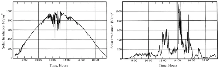
1.1 Solar irradiance variation on typical clear and cloudy days, respectively. 2 1.2 Schematic of a distribution network within the Southern California

Edi-son (SCE) service territory filled with distributed rooftop solar PV in-stallations (red dots), in a projection of a possible near future situation. 3 1.3 Typical voltage profile of a line in a radial distribution feeder. The

voltage magnitude typically drops due to the connected loads and rises due to the power injection from the DG units. . . 4 2.1 Proposed solution strategy for solving OPF. . . 17 2.2 Proposed algorithm for solving OPF (2.11)–(2.12). The details are

ex-plained in Sections 2.3–2.7. . . 18 2.3 Illustration of the branch flow variables . . . 25 2.4 _X is the set of branch flow solutions and ˆ_Y= ˆh(_Y) is the set of relaxed

solutions. The inverse projection hθ is defined in Section V. . . 27

2.5 Model of a phase shifter in line (i, j). . . 42 2.6 Fact 2.7: ˆhis injective on_X. _Xcan be represented by curves in the space

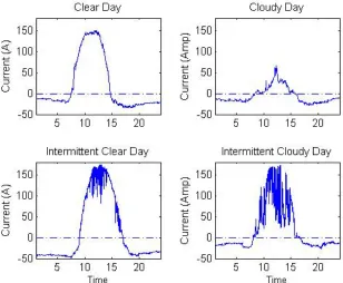
R3m+n+2×[−π, π]n, and Y by the shaded areas (higher dimensional). 56 3.1 Line current measurement at the substation for one of SCE’s lightly

(12)

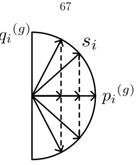
3.2 Two-timescale discretization of a day for switched controllers and in-verters. . . 64 3.3 In order to regulate the voltage, inverters can quickly dispatch reactive

power limited by |q_ig(t)| ≤

q

s2

i −(p g i(t))

2

). . . 67 3.4 Illustration of the dynamic programming approach to solve the slow

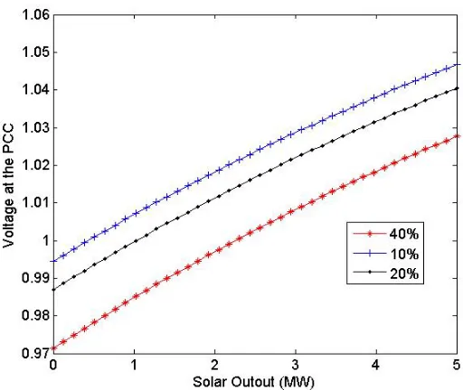
time-scale voltage control problem in a distribution feeder with 4 on/off switched capacitors. . . 70 3.5 Circuit diagram for SCE distribution system. . . 75 3.6 Voltage magnitude at the point of common coupling (PCC) vs solar

output. . . 76 3.7 Illustration of trade-offs in optimal inverter volt/var control problem. . 77 3.8 Optimal inverter reactive power (in KVAR) vs PV output when load is

low. . . 78 3.9 Optimal inverter reactive power (in KVAR) vs PV output when load is

high. . . 78 3.10 Optimal inverter reactive power (in KVAR) vs total load. . . 78 3.11 Schematic diagram of a distribution feeder with high penetration of

Pho-tovoltaics. Bus No. 1 is the substation bus and the 6 loads attached to it model other feeders on this substation. . . 81 3.12 Joint distribution of the normalized solar output level and the

normal-ized load level . . . 82 3.13 Overall power savings in MW, for different load and solar output levels

assuming a 3% voltage drop tolerance. . . 83 4.1 Li∩ Lj for two arbitrary busesi, j in the network and the corresponding

mutual voltage-to-power-injection sensitivity factors Rij, Xij . . . 91

4.2 Two possible network structures . . . 92 4.3 Piecewise linear volt/var control curve discussed in the latest draft of

(13)

4.5 The cost function Ci(qi) corresponding tofi−1 of Figure 4.4. . . 103

5.1 Circuit diagram for SCE distribution system. . . 111 5.2 Dynamics in reactive power injection and voltage magnitude for the case

of a single inverter. . . 113 5.3 Oscillation in voltage profile when all inverters operate. . . 114 5.4 Convergence of the proposed incremental voltage control with different

stepsizes. . . 115 5.5 D2 and D3 both converge . . . 122 5.6 D2 and D3 can be brought back to convergence by changing stepsizes

γg and γp to small enough values. . . 123

5.7 The upper bounds forγg andγp is related by a factor close to theoretical

value max(αi). . . 124

(14)

List of Tables

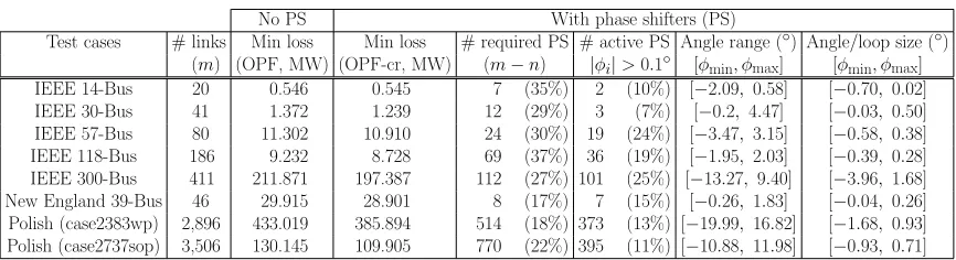
2.1 Notations. . . 24 2.2 Loss minimization. Min loss without phase shifters (PS) was computed

using SDP relaxation of OPF; min loss with phase shifters was computed using SOCP relaxations OPF-cr of OPF-ar. The “(%)” indicates the number of PS as a percentage of #links. . . 50 2.3 Loadability maximization. Max loadability without phase shifters (PS)

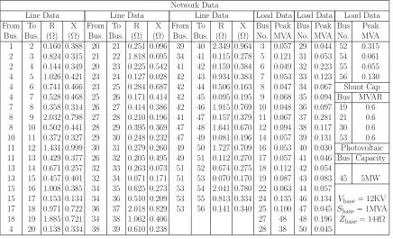
was computed using SDP relaxation of OPF; max loadability with phase shifters was computed using SOCP relaxations OPF-cr of OPF-ar. The “(%)” indicates the number of PS as a percentage of #links. . . 50 3.1 Line impedances, peak spot load KVA, capacitors and PV generation’s

nameplate ratings for the distribution circuit in Figure 3.5. . . 75 3.2 Simulation Results For Some Voltage Tolerance Thresholds . . . 80 3.3 Network of Fig. 3.11: Line impedances, peak spot load KVA, capacitors,

and PV generation’s nameplate ratings. . . 81 3.4 Simulation Results For Some Voltage Tolerance Thresholds . . . 84 4.1 Notations. . . 89 5.1 Network of Fig. 5.1: Line impedances, peak spot load KVA, capacitors,

(15)

Chapter 1 Introduction

As one of the greatest innovations in human history, the power grid is a complex interconnected network of generators, transmission lines, and distribution facilities, designed to deliver electricity from suppliers to consumers. The traditional archi-tecture of the grid consists of large centralized plants, each injecting hundreds of megawatts of power through a mesh of high-voltage transmission lines over long dis-tances, towards low-voltage radial distribution networks that supply electricity to slowly-varying customer loads. With this perspective in mind, distribution networks were originally built to carry power oneway, and to cope with slow changes in loading conditions.

(16)

regu-Figure 1.1: Solar irradiance variation on typical clear and cloudy days, respectively.

lating the voltage and frequency, and maintaining the grid stability and the power quality. In this thesis, we will mostly be focused on energy optimization and steady state voltage regulation in radial distribution networks.

With the increased deployment of intermittent distributed resources, the grid does no longer look like a unidirectional network with few large generators. This challenges the classical design paradigms and motivates the need to implement new operation, protection, and control schemes to cope withfast variation in generation, and bi-directional flows from thousands to millions of new active nodes of all sizes, integrated at every level of the grid. To illustrate the idea, Fig. 1.2 shows the schematic of a real-world distribution network within the Southern California Edison (SCE) service territory, where the red dots represent distributed solar PV installations on this circuit in projection of a possible near future situation.

1.1 Emerging challenges in voltage regulation of

distribution networks

[image:16.612.132.515.83.201.2]

(17)

Figure 1.2: Schematic of a distribution network within the Southern California Edison (SCE) service territory filled with distributed rooftop solar PV installations (red dots), in a projection of a possible near future situation.

taken off-line, posing a treat to the system stability. Utility companies are required to continuously regulate the voltage at the distribution level within the±5% ANSI stan-dard range (0.95 p.u. to 1.05 p.u.), under normal operating conditions. Conventional voltage control equipments, such as switched capacitors and load tap changers, are slow, and work under the assumption that line voltage change slowly and predictably along the feeder. In a traditional unidirectional distribution feeder, the voltage mag-nitude typically drops with the distance from the substation due to line impedance. However, this is no longer true when DG is present. Conversely, when a generator unit is interconnected to a distribution circuit, the real power it injects causes a local voltage rise at the point of connection. If this rise is too large, it may not be feasi-ble to maintain the line voltage within the desired range. Figure 1.3 illustrates the voltage profile of a distribution feeder with a large DG unit. Notice how the voltage drops along the feeder due to the loads until the point of DG interconnection.

(18)

Voltage (p.u.) 1 1.05 0.95

Substation Load Generation

Distance

Figure 1.3: Typical voltage profile of a line in a radial distribution feeder. The voltage magnitude typically drops due to the connected loads and rises due to the power injection from the DG units.

(19)

1.2 DC-AC inverters can takeover the control

As investigated in this thesis, DC-AC inverters can potentially address the challenges in integration of high levels of variable renewable resources, if combined with smart and well-designed control algorithms. Inverters are power electronic devices that are used to couple DC or variable-frequency power sources to the AC grid. In practice, all renewable generators are integrated to the grid through inverter interfaces. In this respect, the primary function of the inverter is to deliver the DC power to the AC side as efficiently as possible. Traditionally, inverters were designed with only the basic control functions necessary to perform this primary task, but increasingly now they are expected to also sense the grid’s health locally, and react accordingly. In addition to frequency conversion and basic real power delivery, inherent control capabilities of these inverters can also help in maintaining the grid stability during under/over voltage events, by injecting or absorbing reactive power into or from the grid, respectively. Although the term “advanced” inverters in the literature may seem to imply a special type of inverter, many of the inverters already deployed today can provide advanced functionality with some minor software upgrades or parameter adjustments.

(20)

and this fast response property makes them a great candidate to cope with rapid voltage fluctuations due to high renewable penetration levels. Indeed, a large number of recent studies [2, 3, 4, 5, 6, 7] in the literature have explored the possibility of utilizing inverter-based distributed generators (DGs) to control voltage fluctuations in distribution systems with high renewable penetration levels, and recognized it as a viable solution. As the share of these intermittent sources increase in the future, inverters are likely to take over more and more of the grid control tasks.

1.3 New opportunities for grid optimization

Since 1960s, mathematical optimization approaches have been developed to increase the power system efficiency. Optimal Power Flow (OPF) is an optimization problem over the decision variables of a power system (e.g., voltage magnitudes at generator buses, status of the capacitor banks, transformer taps, etc), subject to the physical laws of the circuit, and the operational constraints of the network. In practice, these approaches have traditionally been mainly applied to OPF problems at the transmis-sion level. The reason, as discussed earlier, is due to the lack of sufficient monitoring, communication, and controlling elements installed on distribution networks.

But the stakes are high, and the opportunity is there! Indeed, the majority of the 5-8% energy loss in a power system typically occurs in highly resistive lines of distri-bution networks. It is well-known that the installation of DG units can significantly cut these losses by feeding the loads locally and avoiding long distance power trans-fers. Conservation voltage reduction (CVR) can further reduce energy consumption without impacting the customer loads. In short, the utility companies prefer to push customer voltages to the lower half of the ANSI C84.1 range for CVR purposes. Stud-ies have shown that doing so reduces the overall system demand by a factor of about 0.7%–1.0% for every 1% reduction in voltage, depending on the nature of the loads. But this is difficult to achieve with traditional voltage controllers such as capacitor banks, as they tend to create non-smooth voltage profiles.

(21)

re-imagine the optimization at the distribution level. One major change will be the implementation of smart inverter volt/var control functionalities to minimize energy consumption while regulating the voltages within the specified system constraints. In chapter 3, we will formally formulate the inverter var control problem and use the relaxation-based algorithm developed in chapter 2 to solve it. We demonstrate, through experimental studies on two real-world distribution feeders on SCE service territory that the optimal inverter var control algorithms can result in an overall 2%– 4% reduction in distribution network energy consumption by carefully flattening the voltage profile curve (using the continuous var control capability of the inverters) and then lowering it. However, it is important to note that these benefits are achieved at the cost of increasing the internal losses in inverters when they actively participate in volt/var control. In chapter 3, we also provide a model to formally account for this type of loss and weigh it against the overall energy saving benefits in different scenarios. Our findings suggest that, contrary to the common beliefs, there’s no simple solution due to the fact that the components of objective work against each other. The key message is that the optimal inverter var control is a highly non-trivial problem that needs to be properly formulated and rigorously solved. We will see how the additional cost of the internal inverter losses may completely offset the benefits in some scenarios.

1.4 The big picture

(22)

inverter’s role in providing ancillary services to facilitate more reliable integration of renewable resources. Proposed approaches to inverter-based voltage control in distribution networks can be broadly divided into the following three main categories: (i) Approaches that propose a centralized control scheme by solving a global optimal power flow (OPF) problem. These methods implicitly assume an un-derlying complete two-way communication system between a central computing authority and the controlled nodes [4, 11, 12];

(ii) Distributed message-passing algorithms in which communications are lim-ited to neighboring nodes [5, 13, 12, 14];

(iii) Local control methods that require no communications and rely only on local measurements and computations [3, 6, 15]. These include reactive power control based on local real power injection (referred to as Q(P)), power factor control, and the more common voltage based reactive power control (referred to as Q(V)).

In our opinion, solutions at the two ends of this spectrum are more applicable today and should be given a higher priority in research. On one hand, optimal centralized solutions are critical for the purpose of analytical analysis and better understanding of the impact of renewables on the grid. And on the other hand, fully decentralized local control methods are the only approaches available for immediate implementa-tion in today’s distribuimplementa-tion networks, due to the lack of sufficient telecommunicaimplementa-tion infrastructure. It is the goal of this thesis to identify some key problems in these two areas and contribute by providing rigorous theoretical basis for further work.

1.5 Thesis overview and contributions

(23)

1.5.1 Branch Flow Model: relaxations and convexification

In this chapter, we start by providing a general framework for efficiently solving centralized optimization problems in distribution networks. The content is based on the results published in [16, 17, 4, 18]. We propose a branch flow model (BFM) for the analysis and optimization of radial as well as meshed networks. The model is based on the branch power and current flows in addition to nodal voltages, and it leads to a new approach to solving optimal power flow (OPF) problems. It consists of two relaxation steps: the first step eliminates the voltage and current angles and the second step approximates the resulting problem by a conic program that can be solved efficiently. For radial networks, we prove that both relaxation steps are always exact, provided there are no upper bounds on loads. For mesh networks, the conic relaxation is always exact and we provide a simple way to determine if a relaxed solution is globally optimal. We propose a simple method to convexify a mesh network using phase shifters so that both relaxation steps are always exact and OPF for the convexified network can always be solved efficiently for a globally optimal solution. We prove that convexification requires phase shifters only outside a spanning tree of the network graph and their placement depends only on network topology, and not on power flows, generation, loads, or operating constraints. We present simulation results on phase shifter ranges required for the covexification of various IEEE and other test networks.

(24)

1.5.2 Voltage control in distribution systems with high PV

penetration

In this chapter, a practical viewpoint is adopted and the goal is to apply the theoretical results of the previous chapters to study the distribution system level impacts of high-penetration photovoltaic (PV) integration and propose mitigating solutions. The content of this chapter is based on our published work in [4, 21]

We will start by formulating a volt/var optimization problem in distribution net-works and use the relaxation-based algorithm developed in chapter 2 to solve it. We demonstrate, through experimental studies on two real-world distribution feeders on SCE service territory, that the optimal inverter var control algorithms can result in an overall 2%–4% reduction in distribution network energy consumption by carefully flattening the voltage profile curve (using the continuous var control capability of the inverters) and then lowering it. It is important to note that these benefits are achieved at the cost of increasing the internal losses in inverters when they actively participate in volt/var control. Therefore, we include a model to account for this type of loss and weigh it against the overall energy saving benefits in different scenarios. Our findings suggest that, contrary to the common beliefs, there’s no simple solution: the optimal inverter var control is a highly non-trivial problem that needs to be properly formulated and rigorously solved. We will see how the additional cost of the internal inverter losses may completely offset the benefits in some scenarios.

1.5.3 Equilibrium and dynamics of local voltage control in

distribution networks

This chapter is motivated by lack of sufficient theoretical understanding of the be-havior of local voltage control methods in distribution networks. These are the only options available for immediate implementation in today’s distribution networks due to scarcity of the information and the lack of sufficient communication infrastructure. The content is based on our published work in [19].

(25)

decision on the reactive power at a bus depends only on locally measured bus volt-age. These local control algorithms essentially form a closed-loop dynamical system whereby the measured voltage determines the reactive power injection, which in turn affects the voltage. There has been only a limited rigorous treatment of the equilib-rium and dynamical properties of such feedback systems. We show that the dynamical system has a unique equilibrium by interpreting the dynamics as a distributed algo-rithm for solving a certain convex optimization problem whose unique optimal point is the system equilibrium. Moreover, we show that the objective function serves as a Lyapunov function implying global asymptotic stability of the equilibrium. We essen-tially follow a reverse-engineering approach in this chapter, which not only provides a way to characterize the equilibrium, but also suggests a principled way to engineer the control. We then apply the results to study the parameter setting for the piece-wise linear local volt/var control curves proposed in the latest draft of the new IEEE 1547.8 standard document.

1.5.4 Incremental local voltage control algorithms

(26)

(27)

Chapter 2 Branch Flow Model: Relaxations

and Convexification

In this chapter, we propose a branch flow model for the analysis and optimization of mesh as well as radial networks. The model leads to a new approach to solving optimal power flow (OPF) problems that consists of two relaxation steps. The first step eliminates the voltage and current angles and the second step approximates the resulting problem by a conic program that can be solved efficiently. For radial networks, we prove that both relaxation steps are always exact, provided there are no upper bounds on loads. For mesh networks, the conic relaxation is always exact and we provide a simple way to determine if a relaxed solution is globally optimal. We propose a simple method to convexify a mesh network using phase shifters so that both relaxation steps are always exact and OPF for the convexified network can always be solved efficiently for a globally optimal solution. We prove that convexification requires phase shifters only outside a spanning tree of the network graph and their placement depends only on network topology, not on power flows, generation, loads, or operating constraints. We present simulation results on phase shifter ranges required for the covexification of various IEEE and other test networks.

2.1 Background and literature review

(28)

and does not directly deal with power flows on individual branches. A key advantage is the simple linear relationship I = Y V between the nodal current injections I and the bus voltagesV through the admittance matrixY. Instead of nodal variables, the branch flow model focuses on currents and powers on the branches. It has been used mainly for modeling distribution circuits, which tend to be radial, but has received far less attention. In this chapter, we advocate the use of branch flow model for both

radial and mesh networks, and demonstrate how it can be used for optimizing the design and operation of power systems.

(29)

pat-tern. See also [38] for a generalization. These results confirm that radial networks are computationally much simpler. This is important as most distribution systems are radial.

The limitation of semidefinite relaxation for OPF is studied in [39] using mesh networks with 3, 5, and 7 buses. They show that as a line-flow constraint is tightened, the sufficient condition in [12] fails to hold for these examples and the duality gap becomes nonzero. Moreover, the solutions produced by the semidefinite relaxation are physically meaningless in those cases. Indeed, examples of nonconvexity have long been discussed in the literature, e.g., [40, 39, 41]. Hence it is important to develop systematic methods for solving OPF involving mesh networks when convex relaxation fails. See, e.g., [42] for branch-and-bound algorithms for solving OPF when the duality gap is nonzero.

The papers above are all based on the bus injection model. In this chapter, we introduce a branch flow model on which OPF and its relaxations can also be defined. Our model is motivated by a model first proposed by Baran and Wu in [43, 44] for the optimal placement and sizing of switched capacitors in distribution circuits for Volt/VAR control. By recasting their model as a set of linear and quadratic equality constraints, [4, 21] observes that relaxing the quadratic equality constraints to inequality constraints yields a second-order cone program (SOCP). It proves that the SOCP relaxation is exact when there are no upper bounds on the loads. This result is extended here to mesh networks with line limits, and convex, as opposed to linear, objective functions (Theorem 2.1). See also [45, 46] for various convex relaxations of approximations of the Baran-Wu model.

Other branch flow models have also been studied, e.g., in [47, 48, 11], all for radial networks. Indeed, [47] studies a similar model to that in [43, 44], using receiving-end branch powers as variables instead of sending-end branch powers as in [43, 44]. Both [48] and [11] eliminate voltage angles by defining real and imaginary parts of ViVj∗

(30)

injections, [11] solves for the branch flows through an SOCP relaxation for radial networks, though no proof of optimality is provided.

This set of papers [43, 44, 47, 48, 11, 45, 4, 46, 21] all exploit the fact that power flows can be specified by a simple set of linear and quadratic equalities if voltage angles can be eliminated. Phase angles can be relaxed only for radial networks and generally not for mesh networks, as [49] points out for their branch flow model, because cycles in a mesh network impose nonconvex constraints on the optimization variables (similar to the angle recovery condition in our model; see Theorem 2.2 below). For mesh networks, [49] proposes a sequence of SOCP where the nononvex constraints are replaced by their linear approximations and demonstrates the effectiveness of this approach using seven networks. In this chapter we extend the Baran-Wu model from radial to mesh networks and use it to develop a solution strategy for OPF for mesh as well as radial networks, as we now summarize.

2.2 Summary

Our purpose is to develop a formal theory of branch flow model for the analysis and optimization of mesh as well as radial networks. As an illustration, we formulate OPF within this alternative model, propose relaxations, characterize when a relaxed solution is exact, prove that our relaxations are always exact for radial networks when there are no upper bounds on loads but may not be exact for mesh networks, and show how to use phase shifters to convexify a mesh network so that a relaxed solution is always optimal for the convexified network. A similar set of results have been proved in the sequence of papers [12, 36, 37, 35] for the bus injection model, even though the results have distinct characters in each model and the proof techniques are completely different. Indeed, it can be shown that the two models are equivalent and both help deepen our understanding of OPF.

(31)

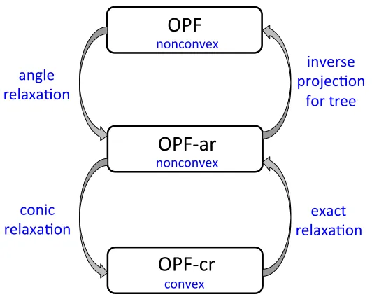
relax-ation steps, as illustrated in Figure 2.1:

• Angle relaxation: relax OPF by eliminating voltage and current angles from the branch flow equations. This yields the (extended) Baran-Wu model and a relaxed problem OPF-ar which is still nonconvex.

• Conic relaxation: relax OPF-ar to a cone program OPF-cr that is convex and hence can be solved efficiently.

!"#$

!"#%&'$

!"#%('$

)*&(+$ '),&*&-./$

0/1)'2)$ 3'.4)(-./$

5.'$+'))$

/./(./1)*$

(./1)*$

&/6,)$ '),&*&-./$

[image:31.612.193.459.242.454.2]

(./0($ '),&*&-./$

Figure 2.1: Proposed solution strategy for solving OPF.

(32)

a mesh network, the angle recovery condition may not hold, and our characterization can be used to check if a relaxed solution yields an optimal solution for OPF.

In Section 2.7 we prove that, by placing phase shifters on some of the branches,

anyrelaxed solution of OPF-ar can be mapped to an optimal solution of OPF for the convexified network, with an optimal cost that is no higher than that of the original network. Phase shifters thus convert an NP-hard problem into a simple problem. Our result implies that when the angle recovery condition holds for a relaxed branch flow solution, not only is the solution optimal for the OPF without phase shifters, but the addition of phase shifters cannot further reduce the optimal cost. On the other hand, when the angle recovery condition is violated, then the convexified network may have a strictly lower optimal cost. Moreover, this benefit can be attained by placing phase shifters only outside an arbitrary spanning tree of the network graph.

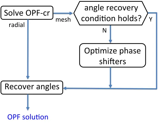
These results suggest an algorithm for solving OPF (2.11)–(2.12) as summarized in Figure 2.1.

Solve OPF-‐cr

Op.mize phase

shi5ers

N

OPF solu.on

Recover angles

radial

[image:32.612.190.457.393.600.2]

angle recovery

condi.on holds?

Y mesh

Figure 2.2: Proposed algorithm for solving OPF (2.11)–(2.12). The details are ex-plained in Sections 2.3–2.7.

(33)

39-bus model of a New England power system and two models of a Polish power system with more than 2,000 buses. Moreover, the placement of these phase shifters depends only on network topology, but not on power flows, generations, loads, or operating constraints. Therefore only one-time deployment cost is required to achieve subsequent simplicity in network operation.

2.3 Branch flow model

Let _R denote the set of real numbers and _C denote the set of complex numbers. A variable without a subscript usually denotes a vector with appropriate components, e.g., s := (si, i = 1, . . . , n), S := (Sij,(i, j) ∈ E). For a complex scalar or vector

a, a∗ denotes its complex conjugate. For a vector a = (a1, . . . , ak), a−i denotes

(a1, . . . , ai−1, ai+1, ak). For a matrix A, At denotes its transpose and A∗ its complex

conjugate transpose. All angles should be interpreted as modulo (being projected into) [−π, π].

2.3.1 Branch flow model

LetG= (N, E) be a connected graph representing a power network, where each node inN represents a bus and each link in E represents a line (condition A1). We index the nodes by i = 0,1, . . . , n. The power network is called radial if its graph G is a tree. For a distribution network, which is typically radial, the root of the tree (node 0) represents the substation bus. For a (generally meshed) transmission network, node 0 represents the slack bus. We use node n to represent ground so that if bus i

has a shunt impedance, then nodei is connected to node n, i.e., (i, n)∈E.

We regard G as a directed graph and adopt the following orientation for con-venience. Pick any spanning tree T := (N, ET) of G rooted at node 0, i.e., T is

connected and ET ⊆ E has n links. All links in ET point away from the root. For

any link in E \ET that is not in the spanning tree T, pick an arbitrary direction.

(34)

if either (i, j) ∈E or (j, i)∈ E (but not both). For each link (i, j)∈ E, we will call nodeitheparentof nodej andj thechildofi. Letπ(j)⊆N be the set of all parents of node j and δ(i)⊆ N the set of all children of node i. Henceforth we will assume without loss of generality that Gand T are directed graphs as described above1.

The basic variables of interest can be defined in terms of G. For each (i, j) ∈E, letIij be the complex current from busesitoj andSij =Pij+iQij be thesending-end

complex power from buses itoj. For each node i∈N, letVi be the complex voltage

on bus i. Let si be the net complex power, which is load minus generation on bus

i. For power flow analysis, we assume si are given. For optimal power flow, VAR

control, or demand response, si are control variables. We use si to denote both the

complex number pi+iqi and the pair (pi, qi) depending on the context. Finally, let

zij =rij+ixij be the complex impedance on the line connecting busesiandj. Recall

that zin represents the shunt impedance on bus i.

Then these quantities satisfy the Ohm’s law:

Vi−Vj = zijIij, ∀(i, j)∈E (2.1)

the definition of branch power flow:

Sij = ViIij∗, ∀(i, j)∈E (2.2)

and power balance at each bus:

X

i∈π(j)

Sij −zij|Iij|2

− X

k∈δ(j)

Sjk = sj, ∀j (2.3)

We will refer to (2.1)–(2.3) as the branch flow model/equations. As customary, we assume that the complex voltageV0 is given and the corresponding complex net load

s0 is a variable. Recall that the cardinality |N|=n+ 1 and letm :=|E|. The branch flow equations (2.1)–(2.3) specify 2m +n + 1 nonlinear equations in 2m +n + 1

1_{The orientation of}_G_and_T _{are different for different spanning trees}_T_{, but we often ignore this}

(35)

complex variables (S, I, V, s0) := (Sij, Iij,(i, j)∈E, Vi, i= 1, . . . , n, s0), when other bus power injections s:= (si, i= 1, . . . , n) are specified.

We will call a solution of (2.1)–(2.3) a branch flow solutionwith respect to a given

s, and denote it by x(s) := (S, I, V, s0). Let X(s)⊆C2m+n+1 be the set of all branch flow solutions with respect to a given s:

X(s) :={x:= (S, I, V, s0)|x solves (2.1)–(2.3) given s}

(2.4)

and let _Xbe the set of all branch flow solutions:

X :=

[

s∈Cn

X(s) (2.5)

For simplicity of exposition, we will often abuse notation and use _X to denote either the set defined in (2.4) or that in (2.5), depending on the context. For instance, _X is used to denote the set in (2.4) for a fixed s in Section 2.6 for power flow analysis, and to denote the set in (2.5) in Section 2.5 for optimal power flow where s itself is also an optimization variable. Similarly for other variables such as x for x(s).

2.3.2 Optimal power flow

Consider the optimal power flow problem where, in addition to (S, I, V, s0), each

si = (pi, qi), i = 1, . . . , n, is also an optimization variable. Let pi := pci −p g i and

qi :=qic−q g

i where pci and qci are the real and reactive power consumption at nodei,

(36)

for i= 0,1, . . . , n,

pg

i ≤p g i ≤p

g i, q

g i ≤q

g

i (2.6)

In particular, any of pg_i, q_ig can be a fixed constant by specifying that pg

i =p g

i and/or

qg i = q

g

i. For instance, in the inverter-based VAR control problem of [4], p g

i are the

fixed (solar) power outputs and the reactive power qg_i are the control variables. For power consumption, we require, for i= 0,1, . . . , n,

pc

i ≤p c i, q

c i ≤q

c

i (2.7)

i.e., there cannot be upper bounds onpc

i, qicfor our proof below to work2. The voltage

magnitudes must be maintained in a tight range: fori= 1, . . . , n,

v_i ≤ |Vi|2 ≤ vi (2.8)

Finally, we impose line flow limits: for all (i, j)∈E,

|Sij| ≤ Sij (2.9)

We allow any objective function that is convex and does not depend on the angles

∠Vi,∠Iij of voltages and currents nor on consumptions pci, qic. For instance, suppose

we aim to minimize real power losses rij|Iij|2, minimize real power generation costs

cip g

i, and maximize energy savings through conservation voltage reduction (CVR).

Then the objective function takes the form (see [4])

X

(i,j)∈E

rij|Iij|2+

X

i∈N

cipgi +

X

i∈N

αi|Vi|2 (2.10)

for some given constants ci, αi ≥ 0. We also allow the cost to be quadratic in real

power as is commonly assumed.

2_{This is equivalent to the “over-satisfaction of load” condition in [12, 36]. As we show in the}

(37)

To simplify notation, let `ij :=|Iij|2 and vi :=|Vi|2. Letsg := (sgi, i= 1, . . . , n) =

(pg_i, qg_i, i = 1, . . . , n) be the power generations, and sc := (sc_i, i = 1, . . . , n) = (pc

i, qci, i = 1, . . . , n) the power consumptions. Let s denote either sc−sg or (sc, sg)

depending on the context. Given a branch flow solution x := x(s) := (S, I, V, s0) with respect to a given s, let ˆy := ˆy(s) := (S, `, v, s0) denote the projection of x that have phase angles _∠Vi,∠Iij eliminated. This defines a projection function ˆh such

that ˆy= ˆh(x), to which we will return in Section 2.4. Then our objective function is

fˆh(x), sg. We assume f(ˆy, sg) is convex (condition A2); in addition, we assumef

is strictly increasing in `ij,(i, j)∈E (condition A3). Finally, let

S := {(v, s0, s)|(v, s0, s) satisfies (2.6)−(2.9)}

All quantities are optimization variables exceptV0, which is given. The optimal power flow problem is

OPF:

min

x,s f

ˆ

h(x), sg (2.11)

subject to x∈_X, (v, s0, s)∈S (2.12)

where _X is defined in (2.5). To avoid triviality, we assume the problem is feasible (condition A4).

The feasible set is specified by the nonlinear branch flow equations and hence OPF (2.11)–(2.12) is in general nonconvex and hard to solve. The goal of this chapter is to propose an efficient way to solve OPF by exploiting the structure of the branch flow model.

2.3.3 Notations and assumptions

(38)

Table 2.1: Notations.

G, T (directed) network graphG and a spanning tree T of G B,BT reduced (and transposed) incidence matrix ofGand the

submatrix corresponding toT

Vi,vi complex voltage on bus iwith vi :=|Vi|2

si =pi+iqi net complex load power on bus i

pi =pci −p g

i net real power equals load minus generation;

qi =qci −q g

i net reactive power equals load minus generation

Iij, `ij complex current from buses i toj with `ij :=|Iij|2

Sij =Pij +iQij complex power from busesi toj (sending-end)

X set of all branch flow solutions that satisfy (2.1)–(2.3) either for some s, or for a given s (sometimes denoted more accurately by_X(s));

ˆ

Y set of all relaxed branch flow solutions that satisfy (2.13)–(2.16) either for a givens or for some s;

Y convex hull of ˆY, i.e., solutions of (2.13)–(2.15) and (2.24);

X, XT set of branch flow solutions that satisfy (2.3), (2.43),

(2.2), for some phase shifter angles φ and for some φ ∈

T⊥;

x= (S, I, V, s0)∈X vectorx of power flow variables ˆ

y = (S, `, v, s0)∈Yˆ and its projection ˆy; ˆ

y = ˆh(x); x=hθ(ˆy) projection mapping ˆy and an inverse hθ

zij =rij +ixij impedance on line connecting busesi and j

f objective function of OPF, of the formfˆh(x), sg

A1 The network graph Gis connected.

A2 The cost function f(ˆy, sg) for optimal power flow is convex. A3 The cost function f(ˆy, sg_{) is strictly increasing in} _`

ij,(i, j)∈E.

A4 The optimal power flow problem OPF (2.11)–(2.12) is feasible.

(39)

2.4 Relaxations and solution strategy

We now describe our solution approach.

2.4.1 Relaxed branch flow model

Substituting (2.2) into (2.1) yieldsVj =Vi−zijSij∗/V

∗

i . Taking the magnitude squared,

we have vj = vi +|zij|2`ij −(zijSij∗ +z

∗

ijSij). Using (2.3) and (2.2) and in terms of

real variables, we therefore have

pj =

X

i∈π(j)

(Pij −rij`ij)−

X

k∈δ(j)

Pjk, ∀j (2.13)

qj =

X

i∈π(j)

(Qij −xij`ij)−

X

k∈δ(j)

Qjk, ∀j (2.14)

vj = vi−2(rijPij+xijQij) + (r2ij +x

2

ij)`ij

∀(i, j)∈E (2.15)

`ij =

P_ij2 +Q2_ij vi

, ∀(i, j)∈E (2.16)

Branch flow variables are shown in figure 2.3. We will refer to (2.13)–(2.16) as the relaxed (branch flow) model/equations and a solution arelaxed (branch flow) so-lution. These equations were first proposed in [43, 44] to model radial distribution circuits. They define a system of equations in the variables (P, Q, `, v, p0, q0) := (Pij, Qij, `ij,(i, j) ∈ E, vi, i = 1, . . . , n, p0, q0). We often use (S, `, v, s0) as a

(40)

hand for (P, Q, `, v, p0, q0). Since we assume the original branch flow model has a solution, the relaxed model also has a solution.

In contrast to the original branch flow equations (2.1)–(2.3), the relaxed equa-tions (2.13)–(2.16) specifies 2(m +n + 1) equations in 3m + n + 2 real variables (P, Q, `, v, p0, q0), for a given s. For a radial network, i.e., G is a tree, m = |E| =

|N| −1 = n. Hence the relaxed system (2.13)–(2.16) specifies 4n+ 2 equations in 4n+ 2 real variables. It is shown in [51] that there are generally multiple solutions, but for practical networks where V0 ' 1 and rij, xij are small p.u., the solution of

(2.13)–(2.16) is unique. Exploiting structural properties of the Jacobian matrix, ef-ficient algorithms have also been proposed in [52] to solve the relaxed branch flow equations.

For a connected mesh network, m = |E| > |N| −1 = n, in which case there are more variables than equations for the relaxed model (2.13)–(2.16), and therefore the solution is generally nonunique. Moreover, some of these solutions may be spurious, i.e., they do not correspond to a solution of the original branch flow equations (2.1)– (2.3).

Indeed, one may consider (S, `, v, s0) as a projection of (S, I, V, s0) where each variableIij orVi is relaxed from a point in the complex plane to a circle with a radius

equal to the distance of the point from the origin. It is therefore not surprising that a relaxed solution of (2.13)–(2.16) may not correspond to any solution of (2.1)–(2.3). The key is whether, given a relaxed solution, we can recover the angles _∠Vi,∠Iij

correctly from it. It is then remarkable that, when G is a tree, indeed the solutions of (2.13)–(2.16) coincide with those of (2.1)–(2.3). Moreover for a general network, (2.13)–(2.16) together with the angle recovery condition in Theorem 2.2 below are indeed equivalent to (2.1)–(2.3), as explained in Section 2.6.

(41)

by ˆh(S, I, V, s0) = (P, Q, `, v, p0, q0) where

Pij = Re Sij, Qij = Im Sij, `ij =|Iij|2 (2.17)

pi = Re si, qi = Im si, vi =|Vi|2 (2.18)

Let _Y ⊆ _C2m+n+1 _{denote the set of all} _y _{:= (}_{S, I, V, s}

0) whose projections are the

ˆ

h

_!

C

2m+n+1

R

3m+n+2

ˆ

Y

X

_{h X}ˆ

_{( )}

Figure 2.4: _X is the set of branch flow solutions and ˆ_Y = ˆh(_Y) is the set of relaxed solutions. The inverse projection hθ is defined in Section V.

relaxed solutions3_:

Y :=

n

y := (S, I, V, s0)|ˆh(y) solves (2.13)–(2.16)

o

(2.19)

Define the projection ˆ_Y:= ˆh(_Y) of _Y onto the space _R2m+n+1 _as

ˆ

Y := { yˆ:= (S, `, v, s0)|yˆsolves (2.13)–(2.16) }

Clearly

X⊆Y and ˆh(X)⊆ˆh(Y) = ˆY

3_{As mentioned earlier, the set defined in (2.19) is strictly speaking}

Y(s) with respect to a fixeds.

To simplify exposition, we abuse notation and useYto denote bothY(s) andSs∈CnY(s), depending

(42)

Their relationship is illustrated in Figure 2.4.

2.4.2 Two relaxations

Consider the OPF with angles relaxed:

OPF-ar:

min

x,s f

ˆ

h(x), sg (2.20)

subject to x∈_Y, (v, s0, s)∈S (2.21)

Clearly, this problem provides a lower bound to the original OPF problem since Y ⊇ X. Since neither ˆh(x) nor the constraints in Y involves angles ∠Vi,∠Iij, this

problem is equivalent to the following

OPF-ar:

min ˆ

y,s f(ˆy, s

g₎ _(2.22)

subject to yˆ∈_Yˆ, (v, s0, s)∈S (2.23)

The feasible set of OPF-ar is specified by a system of linear-quadratic equations. Hence OPF-ar is in general still nonconvex and hard to solve directly. The key to our solution is the observation that the only source of nonconvexity is the quadratic equalities in (2.16). Relax them to inequalities:

`ij ≥

P_ij2 +Q2_ij vi

, (i, j)∈E (2.24)

and define the convex hull _Y⊆_R2m+n+1 _{of ˆ} Y as

(43)

Consider the following relaxation of OPF-ar:

OPF-cr:

min ˆ

y,s f(ˆy, s g

) (2.25)

subject to yˆ∈_Y, (v, s0, s)∈S (2.26)

Clearly OPF-cr provides a lower bound to OPF-ar since _Y⊇_Yˆ.

2.4.3 Solution strategy

In the rest of this chapter, we will prove the following results:

1. OFP-cr is convex. Moreover the conic relaxation is exact so that any optimal solution (ˆycr, scr) of OPF-cr is also optimal for OPF-ar (Section 2.5, Theorem

2.1).

2. Given a solution (ˆyar, sar) of OPF-ar, if the network is radial, then we can

always recover the phase angles_∠Vi,∠Iij uniquely to obtain an optimal solution

(x∗, s∗) of the original OPF (2.11)–(2.12) through an inverse projection (Section

2.6, Theorems 2.2 and 2.3).

3. For a mesh network, an inverse projection may not exist to map the given (ˆyar, sar) to a feasible solution of OPF. In that case, however, the network can

be convexified so that (ˆyar, sar) can indeed be mapped to an optimal solution

of OPF for the convexified network. Moreover, convexification requires phase shifters only on lines outside an arbitrary spanning tree of the network graph (Section 2.7, Theorem 2.4 and Corollary 2).

These results motivate the algorithm in Figure 2.1.

2.5 Exact conic relaxation

(44)

Theorem 2.1. OPF-cr is convex. Moreover, it is exact, i.e., any optimal solution of

OPF-cr is also optimal for OPF-ar.

Proof. The feasible set is convex since the nonlinear inequalities in _Y can be written as the following second order cone constraint:

2Pij

2Qij

`ij −vi

2

≤`ij +vi

Since the objective function is convex, OPF-cr is a conic optimization4_{. To prove} that the relaxation is exact, it suffices to show that any optimal solution of OPF-cr attains equality in (2.24).

Assume for the sake of contradiction that (ˆy∗, s∗) := (S∗, `∗, v∗, sg∗0, sc∗0, sg∗, sc∗) is

optimal for OPF-cr, but a link (i, j)∈Ehas strict inequality, i.e., [v∗]i[`∗]ij >[P∗]ij2+

[Q∗]ij

2

. For some ε > 0 to be determined below, consider another point (˜y,s˜) = ( ˜S,`,˜˜v,s˜g₀,s˜c

0,s˜g,˜sc) defined by:

˜

v = v∗, s˜g = sg∗

˜

`ij = [`∗]ij−ε, `˜−ij = [`∗]−ij

˜

Sij = [S∗]ij −zijε/2, S˜−ij = [S∗]−ij

˜

sc_i = [sc_∗]i+zijε/2, s˜cj = [s c

∗]j +zijε/2

˜

sc₋₍_i,j₎ = [sc_∗]−(i,j)

where a negative index means excluding the indexed element from a vector. Since ˜

`ij = [`∗]ij −ε, (˜y,s˜) has a strictly smaller objective value than (ˆy∗, s∗) because of

assumption A3. If (˜y,˜s) is a feasible point, then it contradicts the optimality of (ˆy∗, s∗).

4_{If the objective function is linear, such as (2.10), then OPF-cr is an SOCP. This is the case}

(45)

It suffices then to check that there exists an ε >0 such that (˜y,˜s) satisfies (2.6)– (2.9), (2.13)–(2.15) and (2.24), and hence is indeed a feasible point. Since (ˆy∗, s∗) is

feasible, (2.6)–(2.9) hold for (˜y,s˜) too. Similarly, (˜y,s˜) satisfies (2.13)–(2.14) at all nodes k 6= i, j and (2.15), (2.24) across all links (k, l) 6= (i, j). We now show that (˜y,s˜) satisfies (2.13)–(2.14) also at nodes i, j, and (2.15), (2.24) across link (i, j):

• Proving (2.13)–(2.14) is equivalent to proving (2.3). At nodei, we have

˜

si = ˜sci −˜s g

i = [s c

∗]i+zijε/2−[sg∗]i

= X

k∈π(i)

([S∗]ki−zki[`∗]ki)−

X

j0_∈_δ₍_i₎_,j0₆₌_j [S∗]ij0

−[S∗]ij +zijε/2

= X

k∈π(i)

˜

Ski−zki`˜ki

− X

j0_∈_δ₍_i₎_,j0₆₌_j ˜

Sij0

−S˜ij +zijε/2

+zijε/2

= X

k∈π(i)

˜

Ski−zki`˜ki

− X

j0_∈_δ₍_i₎ ˜

Sij0

At node j, we have

˜

sj = ˜scj −s˜ g

j = [s c

∗]j +zijε/2−[sg∗]j

= X

i0_∈_π₍_j₎_,i0₆₌_i

([S∗]i0_j −z_i0_j[`_∗]_i0_j) + [S_∗]_ij

−zij[`∗]ij −

X

k∈δ(j)

[S∗]jk +zijε/2

= X

i0_∈_π₍_j₎_,i0₆₌_i

˜

Si0_j −z_i0_j`˜_i0_j

+ ˜Sij +zijε/2

−zij(˜`ij +ε)−

X

k∈δ(j) ˜

Sjk +zijε/2

= X

i0_∈_π₍_j₎

˜

Si0_j −z_i0_j`˜_i0_j

− X

k∈δ(j) ˜

Sjk

Hence (2.13)–(2.14) hold at nodesi, j.

• For (2.9) across link (i, j), we have|S˜ij|2 =|Sij|2−₄ε 2(zij∗Sij +zijSij∗)−ε|zij|2

(46)

|Sij|2 ≤S

2

ij for small enough ε >0.

• For (2.15) across link (i, j), we have

˜

vj = [v∗]i−2(rij[P∗]ij+xij[Q∗]ij)

+(r2_ij+x2_ij)[`∗]ij

= ˜vi−2(rijP˜ij +xijQ˜ij) + (rij2 +x

2

ij)˜`ij

• For (2.24) across link (i, j), we have

˜

vi`˜ij −P˜ij2 −Q˜

2

ij

= [v∗]i([`∗]ij −ε)−([P∗]ij −rijε/2)2

−([Q∗]ij −xijε/2)2

= [v∗]i[`∗]ij −[P∗]2_ij −[Q∗]2_ij

−ε([v∗]i−rij[P∗]ij −xij[Q∗]ij

+ε(r_ij2 +x2_ij)/4

Since [v∗]i[`∗]ij −[P∗]2ij −[Q∗]2ij >0, we can choose an ε > 0 sufficiently small

such that ˜`ij ≥( ˜Pij2 + ˜Q2ij)/˜vi.

This completes the proof.

Remark 2.1. Assumption A3 is used in the proof here to contradict the optimality

of (ˆy∗, sg∗). Instead of A3, if f(ˆy, sg) is nondecreasing in `, the same argument shows that, given an optimal (ˆy∗, sg∗) with a strict inequality [v∗]i[`∗]ij > [P∗]ij

2

+ [Q∗]ij

2

,

one can choose ε > 0 to obtain another optimal point (˜y,s˜g₎ _{that attains equality}

and has a cost f(˜y,s˜g₎_≤ _f_(ˆ_y

∗, sg∗). This implies that, in the absence of A3, there is always an optimal solution of OPF-cr that is also optimal for OPF-ar, even though

it is possible that the convex relaxation OPF-cr may also have other optimal points

with strict inequality that are infeasible for OPF-ar. This is the case for semidefinite

(47)

may also have optimal solutions that are infeasible for the original OPF problem.

2.6 Angle relaxation

Theorem 2.1 justifies solving the convex problem OPF-cr for an optimal solution of OPF-ar. Given a solution (ˆy, s) of OPF-ar, when and how can we recover a solution (x, s) of the original OPF (2.11)–(2.12)? The issue boils down to whether we can recover a solutionx to the branch flow equations (2.1)–(2.3) from ˆy, given any nodal power injections s.

Hence, for the rest of this section, we fix an s. We abuse notation in this section and write x,y, θ,ˆ _X,_Y,_Yˆ instead ofx(s),yˆ(s), θ(s),_X(s),_Y(s),_Yˆ(s), respectively.

2.6.1 Angle recovery condition

Fix a relaxed solution ˆy := (S, `, v, s0)∈Yˆ. Define the (n+ 1)×m incidence matrix

C of Gby

Cie =

            

1 if link e leaves nodei

−1 if link e enters nodei

0 otherwise

(2.27)

The first row ofC corresponds to node 0, the reference bus with a givenV0 =|V0|eiθ0. In this chapter we will only work with them×n reducedincidence matrixB obtained from C by removing the first row (corresponding to V0) and taking the transpose, i.e., for e∈E, i= 1, . . . , n,

Bei =

            

1 if link e leaves node i

−1 if link e enters node i

0 otherwise

(48)

Since G is connected, m ≥ n and rank(B) = n [53]. Fix any spanning tree T = (N, ET) of G. We can assume without loss of generality (possibly after re-labeling

some of the links) that ET consists of links e= 1, . . . , n. Then B can be partitioned

into

B =





BT

B⊥ 

 (2.28)

where then×nsubmatrixBT corresponds to links inT and the (m−n)×nsubmatrix

B⊥ corresponds to links in T⊥ :=G\T.

Let β :=β(ˆy)∈[−π, π]m _{be defined in terms of the given ˆ}_y _by

βij := ∠ vi−zij∗Sij

, (i, j)∈E (2.29)

Write β as

β =





βT

β⊥ 

 (2.30)

where βT is n×1 and β⊥ is (m−n)×1.

Recall the projection mapping ˆh : _C2m+n+1 _→

R3m+n+2 defined in (2.17)–(2.18). For eachθ := (θi, i= 1, . . . , n)∈[−π, π]n, define the inverse projectionhθ :R3m+n+2 → C2m+n+1 byhθ(P, Q, `, v, p0, q0) = (S, I, V, s0) where

Sij := Pij+iQij (2.31)

Iij :=

p

`ij ei(θi−∠Sij) (2.32)

Vi :=

√

vi eiθi (2.33)

s0 := p0+iq0 (2.34)

These mappings are illustrated in Figure 2.4.

(49)

other words, ˆh(_X) consists of exactly those points ˆy ∈ _Yˆ for which there exist θ

such that their inverse projections hθ(ˆh) are in X. Our next key result characterizes

the exact condition under which such an inverse projection exists, and provides an explicit expression for recovering the phase angles _∠Vi,∠Iij from the given ˆy.

A cycle c in G is a set{i1, . . . , ik} of nodes in V such that ij ∼ ij+1 and ik ∼i1, i.e., nodes ij, ij+1 is in c if either (ij, ij+1) ∈ E or (ij+1, ij)∈ E (but not both). We

write e ∈ c when e = (ij ∼ij+1) or e = (ik ∼i1). Let ˜β be the extension of β from directed links to undirected links: if (i, j)∈E then ˜βij :=βij and ˜βji :=−βij.

Theorem 2.2. Let T be any spanning tree of G. Consider a relaxed solution yˆ∈_Yˆ

and the corresponding β defined by (2.29)–(2.30) in terms of yˆ.

1. There exists a unique θ∗ ∈ [−π, π]n such that hθ∗(ˆy) is a branch flow solution

in _X if and only if

B⊥B_T−1βT =β⊥ (2.35)

2. The angle recovery condition (2.35) holds if and only if for every cycle c in G

X

e∈c

˜

βe = 0 (2.36)

3. If (2.35) holds then θ∗ =B_T−1βT.5

Remark 2.2. Given a relaxed solution yˆ := (S, `, v, s0), Theorem 2.2 prescribes a

way to check if a branch flow solution can be recovered from it, and if so, the required

computation. The angle recovery condition (2.35) is a condition on yˆ and depends only on the network topology through the reduced incidence matrix B. The choice of spanning tree T corresponds to choosing n linearly independent rows ofB to form BT

and does not affect the conclusion of the theorem.

Remark 2.3. When it holds, the angle recovery condition (2.36) has a familiar in-terpretation (due to Lemma 1 below): the voltage angle differences (implied byyˆ) sum

(50)

to zero around any cycle.

Remark 2.4. A direct consequence of Theorem 2.2 is that the relaxed branch flow

model (2.13)–(2.16) together with the angle recovery condition (2.35) is equivalent to the original branch flow model (2.1)–(2.3). That is, x satisfies (2.1)–(2.3)if and only if yˆ= ˆh(x) satisfies (2.13)–(2.16) and (2.35).

The proof of Theorem 2.2 relies on the following important lemma that describes when any arbitrary inverse projection hθ(ˆy) is a branch flow solution in X.

Lemma 1. Given yˆ:= (S, `, v, s0) in Yˆ and θ∈[−π, π]n, the vectorhθ(ˆy)defined by

(2.31)–(2.34) is in _X if and only if θ satisfies

θi−θj = ∠ vi−zij∗Sij

, (i, j)∈E (2.37)

Moreover such a θ, if it exists, is unique.

Proof. It is necessary since, from (2.1) and (2.2), we have ViVj∗ = |Vi|2 −z∗ijSij,

yielding θi−θj =∠(vi−zij∗Sij).

For sufficiency, we need to show that (2.13)–(2.16) together with (2.31)–(2.34) and (2.37) implies (2.1)–(2.3). Now (2.13) and (2.14) are equivalent to (2.3). Moreover (2.16) and (2.31)–(2.33) imply (2.2). To prove (2.1), we can substitute (2.2) into (2.37) to get

θi−θj = ∠ vi−zij∗ViIij∗

= _∠ Vi(Vi−zijIij)

∗

Hence

(51)

From (2.15) and (2.2), we have

|Vj|2 = |Vi|2+|zij|2|Iij|2−(zijSij∗ +z

∗

ijSij)

= |Vi|2+|zij|2|Iij|2−(zijVi∗Iij +z∗ijViIij∗)

= |Vi −zijIij|2

This together with (2.38) implies Vj =Vi−zijIij which is (2.1).

The condition (2.37) implies that a branch flow solution can be recovered from a relaxed solution if and only if there exist θ that solves

Bθ = β (2.39)

Since G is connected, m ≥ n and rank(A) = n and hence (2.39) has at most one solution.

Proof of Theorem 2.2. Since m ≥n and rank(B) =n, we can always find n linearly independent rows of B to form a basis. The choice of this basis corresponds to choosing a spanning tree ofG, which always exists sinceGis connected [54, Chapter 5]. Assume without loss of generality that the first n rows is such a basis so that B

and β are partitioned as in (2.28) and (2.30), respectively. Then Lemma 1 implies that there exists a unique θ∗ ∈[−π, π]n such that hθ∗(ˆy) is a branch flow solution in X if and only if θ∗ solves (2.39), i.e.,





BT

B⊥ 

θ =





βT

β⊥ 

 (2.40)

Since T is a spanning tree, the n ×n submatrix BT has a full rank and hence is

invertible. Therefore,θ∗ =B_T−1βT. Moreover, (2.40) has a unique solution if and only

if B⊥θ∗ =B⊥B_T−1βT =β⊥.

(52)

0. Let T(i j) denote the unique path from node i to node j in T; in particular,

T(0 j) consists of links all with the same orientation as the path andT(j 0) of links all with the opposite orientation. Then it can be verified directly that B−_T1 is defined by [54, Chapter 5]

B_T−1_ei :=



 

 

−1 if linke is in T(0 i)

0 otherwise

Then B_T−1βT represents the (negative of the) sum of angle differences on the path

T(0 i) for each node i∈T:

B_T−1βT

i =

X

e

B_T−1_ie[βT]e = −

X

e∈T(0 i) [βT]e

Hence B⊥B_T−1βT is the sum of voltage angle differences from node i to node j along

the unique path in T, for every link (i, j)∈E\ET not in the tree T. To see this, we

have, for each link e:= (i, j)∈E\ET,

B⊥B_T−1βT

e =

B_T−1βT

i−

B_T−1βT

j

= X

e0_∈_T₍₀ _j₎

[βT]_e0 −

X

e0_∈_T₍₀ _i₎ [βT]_e0

Since

X

e0_∈_T₍₀ _j₎

[βT]_e0 = −

X

e0_∈_T₍_j ₀₎

h

˜

βT

i

e0

the angle recovery condition (2.35) is equivalent to

X

e0_∈_T₍₀ _i₎

[βT]e0 + [β⊥]_ij + X

e0_∈_T₍_j ₀₎

h ˜ βT i e0 = X

e0_∈_c₍_i,j₎ ˜

(53)

where c(i, j) denotes the unique basis cycle (with respect to T) associated with each link (i, j) not in T [54, Chapter 5]. Hence (2.35) is equivalent to (2.36) on all basis cycles, and therefore it is equivalent to (2.36) on all cycles.

2.6.2 Angle recovery algorithms

Theorem 2.2 suggests a centralized method to compute a branch flow solution from a relaxed solution.

Algorithm 1: centralized angle recovery. Given a relaxed solution ˆy ∈_Yˆ, 1. Choose any n basis rows of B and form BT and B⊥.

2. Compute β from ˆy and check if B⊥B_T−1βT =β⊥.

3. If not, then ˆy6∈ˆh(_X); stop. 4. Otherwise, compute θ∗ =B_T−1βT.

5. Compute hθ∗(ˆy)∈X through (2.31)–(2.34).

Theorem 2.2 guarantees that hθ∗(ˆy), if it exists, is the unique branch flow solution of (2.1)–(2.3) corresponding to (whose projection is) ˆy.

The relations (2.2) and (2.37) motivate an alternative iterative procedure to com-pute the angles _∠Iij, ∠Vi, and hence a branch flow solution. This procedure is more

amenable to a distributed implementation.

Algorithm 2: distributed angle recovery. Given a relaxed solution ˆy ∈_Yˆ, 1. Choose any spanning tree T of G rooted at node 0.

2. Forj = 0,1, . . . , n(i.e., as index j ranges over the treeT, starting from the root and in the order of breadth-first search), for all descendents k∈δ(j), set

∠Ijk := ∠Vj−∠Sjk (2.41)

(54)

3. For each link (j, k) ∈E \ET not in the spanning tree, node j is an additional

parent of k in addition to k’s parent in the spanning tree from which _∠Vk has

already been computed in Step 2.

(a) Compute current angle _∠Ijk using (2.41).

(b) Compute a new voltage angle θ_kj using the new parent j and (2.42). If

θj_k6=_∠Vk, then angle recovery has failed and ˆy is spurious.

If the angle recovery procedure succeeds in Step 3, then ˆytogether with these angles

∠Vk,∠Ijk are indeed a branch flow solution. Otherwise, a link (j, k) not in the tree

T has been identified where condition (2.36) is violated over the basis cycle c(j, k) associated with link (j, k).

2.6.3 Radial networks

Recall that all relaxed solutions in ˆ_Y\hˆ(_X) are spurious. Our next key result shows that, for radial network, ˆh(_X) = ˆ_Y and hence angle relaxation is always exact in the sense that there is always a unique inverse projection that maps any relaxed solution ˆ

y to a branch flow solution in _X(even though _X6=_Y).

Theorem 2.3. Suppose G=T is a tree. Then

1. ˆh(_X) = ˆ_Y.

2. given any yˆ, θ∗ :=B−1β always exists and is the unique phase angle vector such that hθ∗(ˆy)∈X.

Proof. When G =T is a tree, m =n and hence B = BT and β = βT. Moreover B

is n×n and of full rank. Therefore θ∗ = B−1β always exists and, by Theorem 2.2,

hθ∗(ˆy) is the unique branch flow solution in X whose projection is ˆy. Since this holds for any arbitrary ˆy∈_Yˆ, ˆ_Y= ˆh(_X).

Optimization and Control of Power Flow in Distribution Networks