An Approach to Solve a Possibilistic Linear Programming Problem

(1)

http://dx.doi.org/10.4236/am.2014.52024

An Approach to Solve a Possibilistic Linear Programming

Problem

Ritika Chopra1, Ratnesh R. Saxena2 1

Department of Mathematics, Delhi University, Delhi, India

2

Department of Mathematics, DeenDayalUpadhyay College, Delhi University, Delhi, India Email:[email protected], [email protected]

Received May 30, 2013; revised June 30, 2013; accepted July 7, 2013

Copyright © 2014 Ritika Chopra, Ratnesh R. Saxena. This is an open access article distributed under the Creative Commons Attribu-tion License, which permits unrestricted use, distribuAttribu-tion, and reproducAttribu-tion in any medium, provided the original work is properly cited. In accordance of the Creative Commons Attribution License all Copyrights © 2014 are reserved for SCIRP and the owner of the intellectual property Ritika Chopra, Ratnesh R. Saxena. All Copyright © 2014 are guarded by law and by SCIRP as a guardian.

ABSTRACT

The objective of the paper is to deal with a kind of possibilistic linear programming (PLP) problem involving multiple objectives of conflicting nature. In particular, we have considered a multi objective linear programming (MOLP) problem whose objective is to simultaneously minimize cost and maximize profit in a supply chain where cost and profit coefficients, and related parameters such as available supply, forecast demand and budget are fuzzy with trapezoidal fuzzy numbers. An example is given to illustrate the strategy used to solve the afore-said PLP problem.

KEYWORDS

Multi Objective Linear Programming Problem; Fuzzy Set Theory; Trapezoidal Fuzzy Numbers; Possibilistic Linear Programming Problem

1. Introduction

In a supply chain, a distribution planning decision (DPD) problem involves optimizing the distribution plan for transporting goods from a set of sources to a set of destinations. In most real world problems, the decision maker has to often deal with several objectives, which might be conflicting in nature. Also, available supply, forecast demand and related cost/time/profit coefficients, are often imprecise (fuzzy) because of incomplete or (and) un- available information. Fuzzy set theory was presented by Zadeh [1]. It was taken ahead when Bellman and Za- deh [2] proposed the concept of decision making in fuzzy environments. After the pioneering work on fuzzy linear programming by Zimmermann [3], several kinds of fuzzy linear programming problems have appeared in the literature and different methods have been proposed to solve such problems.

Furthermore, Zimmermann [4] extended his FLP method to a multi-objective linear programming (MOLP) problem. Related studies on solving DPD problems with multiple fuzzy objectives included Hussein [5] and Abd El-Wahed [6]. Moreover, Lai and Hwang [7] developed an auxiliary MOLP model for solving PLP problems with imprecise objective and/or constraint coefficients with triangular distributions. Tien-Fu Liang [8] in- tegrated the available concepts to solve multi-objective DPD problems involving imprecise available supply, forecast demand and unit cost/time coefficients with triangular possibility distributions.

(2)

The proposed methodology can be applied to various real world multi objective problems such as assignment problems, transportation problems and many more such problems in which the information is given in the form of trapezoidal/triangular/interval possibility distributions.

2. Notations

Index sets

 i index for source, for all i=1, 2,,m

 j index for destination, for all j=1, 2,,n

 g index for objectives, for g = 1, 2 Decision variables

 xij units distributed from source i to destination j (units)

Objective functions

 z₁ total distribution costs ($)

 z2 total profit ($)

Parameters

 c_ij distribution cost per unit delivered from source i to destination j ($/unit)

 p_ij profit per unit delivered from source i to destination j ($/unit)

 S_i total available supply for each source i (units)

 Dj total forecast demand of each destination j (units)

 B total budget ($)

3. Problem Description

A general multi objective distribution programming problem aims to determine the right plan for distributing a homogeneous commodity from m sources to n destinations. Each source has an available supply of the commodity to distribute to various destinations, and each destination has a forecast demand of the commodity to be received from various sources. The available supply for each source, the forecast demand for each destination, and related cost/profit coefficients are generally imprecise over the planning horizon due to incomplete and/or unobtainable information. The proposed PLP method aims to simultaneously minimize the total distribution costs and maximize the total profit with reference to available supply constraint at each source, forecast demand constraint at each destination and the total budget constraint. This work focuses on developing an interactive PLP method for optimizing the distribution plan in uncertain environments.

Thus, all the objectives are imprecise thereby incorporating the variations in the decision maker’s judgments relating to the solutions of the multi objective optimization problems in a framework of fuzzy aspiration levels. The pattern of trapezoidal possibility distribution is adopted to represent the imprecise objective functions and related imprecise numbers. All of the objective functions and the constraints are linear and the cost and profit on a given route are directly proportional to the units distributed.

Mathematically,

 

1 1 1 min

m n

ij ij i j

z c x

= =

=

∑∑

(3.1)

 

2 1 1 max

m n

ij ij i j

x p z

= =

=

∑∑

(3.2)

Subject to



1

1, 2, ,

n

ij i j

x S i m

=

≤ ∀ =

∑

 (3.3)



1

1, 2, ,

m ij j i

x D j n

=

≤ ∀ =

(3)



1 1

m n

ij ij i j

c x B

= =

≤

∑∑

_(3.5)

0 1, 2, , 1, 2, ,

ij

x ≥ ∀ =i  m ∀ =j n

Here cij , pij , Si , Dj , B are all fuzzy with trapezoidal possibility distribution ∀ =i 1, 2,,m ,

1, 2, ,

j n

∀ =  .

4. Methodology

Since all the given parameters are assumed to be fuzzy with trapezoidal possibility distribution so, in particular, cost coefficient cij is written as 

(

, , ,

)

o m m p ij ij ij ij ij

c = c c c c (see Figure 1), where cijo is the most optimistic value

that has a very low likelihood of belonging to the set of available values ( degree of association = 0), m, m ij ij

c c

 

  is the interval of most possible value that definitely belongs to the set of available values (degree of association = 1, if normalized), cijp is the most pessimistic value that has a very low likelihood of belonging to the set of

avail-able values ( degree of association = 0).

Geometrically, the imprecise objective function for cost is fully defined by four prominent points

( )

1, 0

o

z ,

( )

1 ,1

m

z ,

( )

1,1

m

z and

( )

1, 0

p

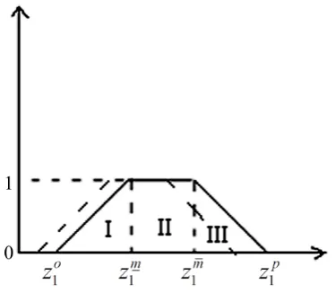
z . Since the objective is to minimize cost so in order to get a minimum cost we shift the trapezium to the left ensuring higher possibility of getting a low value of cost. Thus, we aim to simultaneously minimize 1

p m

z −z .

[image:3.595.219.409.360.526.2]

Therefore, the fuzzy cost objective is broken down into the following four crisp objectives

)

14 1 1 min m n p m

ij ij ij i j

z c c x

= =

−

=

∑∑

(4.4)

Similarly, profit coefficient pij is written as 

(

, , ,

)

p m m o ij pij ij ij ij

p = p p p , where pijo is the most optimistic value

that has a very low likelihood of belonging to the set of available values (degree of association = 0), pijm,pijm

is the interval of most possible value that definitely belongs to the set of available values (degree of association = 1, if normalized), pijp is the most pessimistic value that has a very low likelihood of belonging to the set of

available values ( degree of association = 0).

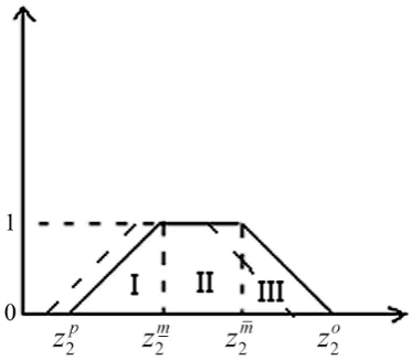
Geometrically, the imprecise objective function for profit is fully defined by four prominent points

( )

2 2

)

n

o m m p

ij i i i i

j

x w S _β w S _β w S _β w S _β i m

=

≤ + + + ∀ =

∑

 (4.9)

1 , 2 , 3 , 4 ,

1

1, 2, ,

m

o m m p ij i i i i i

x w D_β w D_β w D _β w D_β j n

=

≥ + + + ∀ =

∑



The budget constraint is an inequality with fuzzy numbers on both the sides, so fuzzy ranking method is adopted to defuzzify the constraint. Accordingly, if the minimum acceptable possibility is specified by the DM, the corresponding auxiliary crisp inequality can be represented as

1 1

m n

m m

ij ij i j

c x B_β

= =

≤

∑∑

(4.11)

1 1

m n

m m

ij ij i j

c x B_β

= =

≤

∑∑

(4.12)

1 1

m n

o o

ij ij i j

c x B_β

= =

≤

∑∑

(4.13)

1 1

m n

p p

ij ij i j

c x B_β

= =

≤

∑∑

(4.14)

)

14 min 1 1 14 max 1 1

PIS p m NIS p m

)

24 max 2 2 24 min 2 2

PIS o m NIS o m

z = z −z z = z −z

Note that PIS is the optimum value of the objective over the given set of constraints when all the other objec-tives are ignored and NIS is the optimum value of its dual over the given set of constraints. Furthermore, the corresponding linear membership function for each of the new objective functions of the auxiliary MOLP prob-lem is defined by

( )

11 11

11 11 11 11 11

11 11 11 11 1 if if 0 if PIS NIS PIS NIS NIS PIS NIS z z z z

f z z z z

z z z z  ≤  −  =_ ≤ ≤ −   _≤  (4.15)

( )

12 12 12 12

12 12 12 12 12

12 12 12 12 1 if if 0 if PIS NIS NIS PIS NIS PIS NIS z z z z

f z z z z

(6)

Linear membership functions for objective functions (4.4) and (4.7) are similar to the linear membership function for objective function (4.1) given by the Equation (4.15) and the linear membership function for objective functions (4.3), (4.5), (4.6) and (4.8) are similar to the linear membership function for objective function (4.2) given by the Equation (4.16).

Finally, aggregate all fuzzy sets using the minimum operator of fuzzy decision making concept. Let λ be the auxiliary variable

(

0≤ ≤λ 1

)

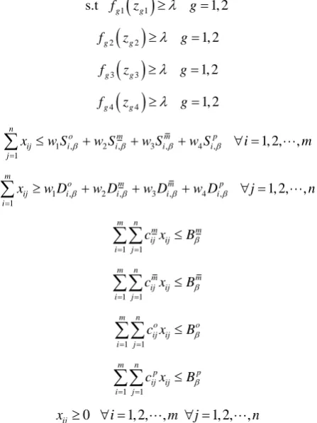
, which represents the degree of satisfaction of the decision maker. Thus, we aim to maximize the decision maker’s satisfaction, which is nothing but the minimum of the membership functions corresponding to the objectives [2,4]. Then, the corresponding single objective linear programming problem is max λ

4 4 1, 2

g g

f z ≥λ g=

1 , 2 , 3 , 4 , 1

1, 2, ,

n

o m m p

ij i i i i

j

x w S _β w S _β w S _β w S _β i m

=

≤ + + + ∀ =

∑



1 , 2 , 3 , 4 ,

1

1, 2, ,

m

o m m p ij i i i i i

x w D _β w D_β w D _β w D_β j n

=

≥ + + + ∀ =

∑



1 1

m n

m m

ij ij i j

c x B_β

= =

≤

∑∑

1 1

m n

m m

ij ij i j

c x B_β

= =

≤

∑∑

1 1

m n

o o

ij ij i j

c x B_β

= =

≤

∑∑

1 1

m n

p p

ij ij i j

c x B_β

= =

≤

∑∑

0 1, 2, , 1, 2, ,

ij

x ≥ ∀ =i m ∀ =j n

The above problem is a crisp single objective linear programming problem which can easily be solved using MATLAB.

5. Numerical Illustration

Consider the problem given in Table 1.

[image:6.595.201.425.202.501.2] [image:6.595.84.514.612.723.2]

Also, the total budget, B=$ 132000,138000,144000,148000

(

)

.

Table 1. Problem in consideration.

A B C D Supply (in thousand)

1 (0.6, 0.7, 0.8, 0.9)

*

(0.1, 0.2, 0.3, 0.4)**

(2.4, 2.7, 3.2, 3.5) (1.0, 1.4, 1.7, 2.0)

(1.8, 2.0, 2.1, 2.3) (1.0, 1.3, 1.5, 1.6)

(1.5, 1.7, 1.9, 2.0) (0.7, 0.8, 0.9, 1.0)

(17.2, 17.8, 18.5, 19.2)

2 (1.1, 1.2, 1.3, 1.4) (0.4, 0.5, 0.6, 0.7)

(3.1, 3.4, 3.8, 4.1) (1.5, 1.7, 2.0, 2.1)

(1.4, 1.5, 1.6, 1.7) (0.8, 0.9, 1.0, 1.1)

(2.2, 2.4, 2.6, 2.7) (1.0, 1.3, 1.6, 1.8)

(22.6, 23.7, 24.6, 25.8)

3 (1.5, 1.7, 1.9, 2.0) (0.6, 0.8, 1.0, 1.1)

(3.1, 3.4, 3.6, 3.9) (1.4, 1.7, 1.9, 2.2)

(2.1, 2.4, 2.5, 2.7) (1.3, 1.4, 1.5, 1.7)

(0.8, 0.9, 1.0, 1.1) (0.1, 0.2, 0.3, 0.4)

(12.6, 12.9, 13.2, 13.6)

Demand

in thousand (11.2, 11.8, 12.1, 12.6) (5.4, 5.7, 6.1, 6.4) (14.8, 15.7, 16.3, 16.8) (19, 19.5, 20.3, 20.8)

*

(7)

[image:7.595.160.436.99.204.2]

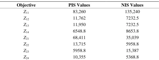
Table 2. PIS and NIS values of the objectives.

Objective PIS Values NIS Values

Z11 83,260 135,240

Z12 11,762 7232.5

Z13 11,950 7232.5

Z14 6548.8 8653.8

Z21 68,411 35,039

Z22 13,715 5958.8

Z23 5958.8 15,387

Z24 10,355 5368.8

First, formulate the original multi-objective fuzzy problem using Equations (3.1) to (3.5). Then, develop the new objective functions for the new crisp multi-objective problem using Equations (4.1) to (4.8). Further, defuzzify fuzzy constraints to get crisp constraints using Equations (4.9) to (4.14) at β =0 assuming w1=w4=1 8

and w2=w3=3 8.

Get the PIS and NIS values (given in Table 2) corresponding to all the crisp objectives.

Additionally, the corresponding linear membership function for each of the fuzzy objectives in the auxiliary MOLP can be defined using Equations (4.15) and (4.16). Finally, the auxiliary MOLP can be converted to an equivalent LP model using the minimum operator to aggregate all fuzzy sets. This LP is then solved using MATLAB.

The solutions are imprecise and have trapezoidal possibility distribution, and overall degree of decision maker satisfaction is 0.9686. Thus, the optimal plan by the above method is as follows:

11 08892, 12 01123, 13 00000, 14 07548

x = x = x = x =

21 03045, 22 04066, 23 15950, 24 00000

x = x = x = x =

31 00000, 32 00711, 33 00000, 34 12352

x = x = x = x =



₍

₎

1 69723, 77026,84890,91439

z =



₍

₎

2 29604,35858, 42336, 48071

z =

6. CONCLUSIONS

This work develops an interactive method for solving multi-objective problems with imprecise available supply, forecast demand and unit cost/profit coefficients with trapezoidal possibility distributions. The model designed here aims to simultaneously minimize the total distribution costs and maximize the total profit with reference to available supply at each source, as well as forecast demand constraints at each destination and the total budget constraint.

Also, the algorithm provides a systematic framework that facilitates the decision-making process, enabling a DM to interactively modify the imprecise data and related parameters until a set of satisfactory solutions is ob-tained. As the value of the parameter β is varied over the interval [0,1], a different optimal feasible solution is obtained. Thus, the DM can choose from a set of optimal solutions, the one which suits the DM most. The table below shows the value of λ for different values of β.

β Λ

0 0.9686

0.1 0.9731

0.2 0.9717

0.3 0.9625

0.4 0.9720

0.5 0.9656

0.6 0.7613

0.7 0.7176

0.8 0.9450

(8)

The method developed can be easily applied to any real world problem with trapezoidal/triangular/interval distributions such as distribution planning decision problems, assignment problems, job allocation problem and more such problems. The method described by Lai and Hwang is a special case of the algorithm described above. Lai and Hwang have considered triangular possibility distribution with both the objectives to be minimized, so if in the algorithm described above, we take zmg =zmg, for g = 1, 2 and both the imprecise objectives are converted

to crisp objectives as in Equations (4.1) to (4.4) then we get the method described by Lai and Hwang. The method described in this paper has an edge over Lai and Hwang method as the method described in the paper cov- ers a broader range of problems.

REFERENCES

[1] L. A. Zadeh, “Fuzzy Sets as a Basis for a Theory of Possibility,” FuzzySetsandSystems, Vol. 1, 1978, pp. 3-28.

[2] R. E. Bellman and L. A. Zadeh, “Decision-Making in a Fuzzy Environment,” ManagementScience, Vol. 17, 1970, pp. 141- 164.

[3] H.-J. Zimmermann, “Description and Optimization of Fuzzy Systems,” InternationalJournalofGeneralSystems, Vol. 2, 1976, pp. 209-215.

[4] H.-J. Zimmermann, “Fuzzy Programming and Linear Programming with Several Objective Functions,” FuzzySetsandSystems, Vol. 1, 1978, pp. 45-56. http://dx.doi.org/10.1016/0165-0114(78)90031-3

[5] M. L. Hussein, “Complete Solutions of Multiple Objective Transportation Problems with Possibilistic Coefficients,” FuzzySets andSystems, Vol. 93, 1998, pp. 293-299.

[6] W. F. Abd El-Washed, “A Multi-Objective Transportation Problem under Fuzziness,” FuzzySetsandSystems, Vol. 117, 2001, pp. 27-33.

[7] Y. J. Lai and C. L. Hwang, “A New Approach to Some Possibilistic Linear Programming Problem,” FuzzySetsandSystems, Vol. 49, 1992, pp. 121-133.