http://dx.doi.org/10.4236/jhepgc.2016.21013
Does a Randall-Sundrum Brane World
Effective Potential Influence Axion Walls
Helping to Form a Cosmological Constant
Affecting Inflation?
Andrew Walcott Beckwith
Chongqing University Huxi Campus, Chongqing, China
Received 8 December 2015; accepted 26 January 2016; published 29 January 2016
Copyright © 2016 by author and Scientific Research Publishing Inc.
This work is licensed under the Creative Commons Attribution International License (CC BY). http://creativecommons.org/licenses/by/4.0/
Abstract
In 2003, Guth posed the following question in a KITP seminar in UCSB. Namely “Even if there exist 101000 vacuum states produced by String theory, does inflation produce overwhelmingly one pre-ferred type of vacuum states over the other possible types of vacuum states”? This document tries to answer how a preferred vacuum state could be produced, and by what sort of process. We con-struct a di quark condensate leading to a cosmological constant in line with known physical ob-servations. We use a phase transition bridge from a tilted washboard potential to the chaotic in-flationary model pioneered by Guth which is congruent with the slow roll criteria. This permits criteria for initiation of graviton production from a domain wall formed after a transition to a chaotic inflationary potential. It also permits investigation of if or not axion wall contributions to inflation are necessary. If we reject an explicit axion mass drop off to infinitesimal values at high temperatures, we may use the Bogomolnyi inequality to rescale and reset initial conditions for the chaotic inflationary potential. Then the Randall-Sundrum brane world effective potential deli-neates the end of the dominant role of di quarks, and the beginning of inflation. And perhaps an-swers Freeman Dysons contention that Graviton production is unlikely given present astrophysi-cal constraints upon detector systems. We end this with a description in the last appendix entry, Appendix VI, as to why, given the emphasis upon di quarks, as to the usefulness of using times be-fore Planck time interval as to modeling our physical system and its importance as to emergent field structures used for cosmological modeling.
Keywords
1. Introduction
It is well known through conventional calculations via QCD that there is a huge disconnection between what is calculated for a cosmological constant [1], and the de facto observed phenomenological data which purports to support a cosmological constant far lower in magnitude than what is presumed to be an artifact of vacuum pola-rization [2]. This paper in part is an answer to this odd divergence and a summary of a different tack to giving a bound to the cosmological constant problem than one supplied by conventional applications of QCD. I contend that not only a difference would take on the cosmological constant yield dividends, but it would also yield an experimentally falsifiable model as to graviton production, as an answer to Freeman Dysons challenge to the as-trophysics community to come up with detector schemes realistically capable of detecting spin two gravitons with our present level of detector technology.
As a general point, when we say S.H.O. I am referring to the acronym of simple harmonic oscillator. This pa-per is dedicated to physics way beyond the S.H.O. (simple harmonic oscillator) approximation and is dedicated to the premise that nonlinear contributions, which are not fully treated in the conventional literature are of deci-sive importance and this paper is a first attempt to include in effects which are often neglected for the same of convenience.
Note also that an acronym WKB is referred to as a semi-classical tunneling approximation in this paper. Semi-classical approximations abound all over physics, and what we are saying is that the construction we are emphasizing allows us to incorporate more quantum mechanical procedures in our treatment of cosmology. The reason for refinements of our protocol about tunneling, as in the initial phases of cosmology lies in our treatment of what is known about zero point fluctuations, which will be brought up next. We in looking at quantum tunne-ling, as in the WKB idea, and it is a way to form vacuum states, initially, in cosmology and also the concept of a vacuum energy density value, which will be the reason for Equation (1) in the paper below. More about the WKB approximation will be in the 2nd to last appendix entry of this document.
The vacuum state idea is brought up, in our document because a quantum state is said to be a vacuum state if the expectation value of the Hamiltonian in a given theory is a local minimum (the Hamiltonian of course being part of the data that defines the theory). We do not necessarily have a Hamiltonian for our modeling of cosmol-ogy, although both loop quantum gravity and Wheeler De Witt theory do refer to cosmological states, although incompletely. Needless to state, if we can define a Hamiltonian for cosmological conditions, not impossible to do, then we can go to the next idea, which is that of a vacuum energy density, which is one of the biggest prob-lems in physics today. To a large degree, this document is an attempt to explain what are the consequences of extremely large theoretically calculated vacuum energy density values, and how to ameliorate the serious prob-lems such calculations bring to the study of cosmology.
Zero point fluctuations of quantum fields contribute to an enormous vacuum energy density value ρvacuum
But the reality as seen in solar system based measurements and then in galactic astrophysics data sets have lead to a de facto observed [3]
56 2 29 3
vacuum
10− cm− ρ 10− g cm−
Λ ≤ ⇔ ≤ ⋅ (1)
What we are doing is to give a physical model as to what could be an alternative mechanism physically to the vacuum fluctuation model used in QCD calculations to give a bound to the cosmological constant which avoids having a value roughly 10120 times too large [1]. In addition, this same value included in the cosmological con-stant model would help give an upper bound to graviton production in branes [4] which is a subject which will be done according to putting in the absolute magnitude of the cosmological constant in to a brane world bound to graviton production in a de Sitter, and ANTI de Sitter cosmological metric model [4] [5].
Recent field theory calculations have lowered the overshoot factor to being of the order of 1043 times larger than what is inferred experimentally [6]. This is a significant improvement, but still beggars the question as to what is really needed to get the calculated results in line with known experimental data as referred to in Equation (1) above.
The model which in the end I turned to is similar in part to what was attempted by Weinberg et al. in the early 1980s [7], with one tunneling event through a potential barrier. This was finally discarded, and what I am doing now is to in part re introduce part of the same idea but with a different scalar potential field than was attempted by Weinberg nearly two decades ago.
a tilted Washboard potential for a scalar field [8]-[10]. I am using this method in part for just ONE tunneling event, plus a different constituent scalar field than used by either Weinberg or Abbot to try to get a more realistic value for the cosmological constant.
QCD is the theory of quantum chromodynamics, which is well understood. What we are doing is to try to make QCD as commensurate to quantum gravity, and quantum gravity via the idea of use of di quarks, which show up in this paper.
If as I suspect traditional QCD calculations have missed any essential details, it is in a di quark condensate as a template [11] for a nucleation of initial states contributing to inflation as viewed by Guth, et al. [12] in their papers. In addition, partly for reasons presented in this document, I also believe that the methodology I tried to refine from Abbot’s initial paper, as presented, is useful as a template for synthesis of gravitons. This is also due in part to Axion fields described as a “squeezer” to a di quark condensate [11] [13].
We link an initial di quark configuration to instantons, spalererons, and the early universe. Since spalerons are not well understood, this will necessitate a discussion of spalerons and a thermal bath of temperature T [14]. It is also noteworthy that the bridge between the two potential systems mentioned in this document comes from in-creasing temperature removing a (1-cos {phi}) phase contribution to a tilted potential to what is an eventual typ-ical Guth style quartic potential [15]. Disappearance of axion walls, or their equivalent would be in tandem with increase of temperature, leading to conditions at the start of start of inflation which would at that time, past the first instant of Planck time, match necessary and sufficient conditions as to slow roll potential systems used in early universe cosmology.
We argue all of this will set up conditions for describing in detail an effective cosmological constant contribu-tion to brane world produccontribu-tion of gravitons in the early universe. This will be done, assuming that the final input of a cosmological constant is significantly less than what the initial cosmological tilted well potential would give, effectively leading to a large burst of gravitons in an early universe.
Doing this though will necessitate an additional fifth dimension. Usually in mathematics, this is done via the circle group, denoted by T (or by ), is the multiplicative group of all complex numbers with absolute value 1. The name comes from the fact that these numbers lie on the unit circle in the complex plane.
{
z : z 1 .}
= ∈ =
(1a)
The circle group forms a subgroup of C×, the multiplicative group of all nonzero complex numbers. Since C×
is Abelian, it follows that T is as well.
The notation T for the circle group stems from the fact that Tn (the direct product of T with itself n times) is geometrically an n-torus. The circle group is then a 1-torus. As electromagnetism can essentially be formulated as a gauge theory on a fiber bundle, the circle bundle, with gauge group U (1). Once this geometrical interpreta-tion is understood, it is relatively straightforward to replace U (1) by a general Lie group. Such generalizations are often called Yang-Mills theories. If a distinction is drawn, then it is that Yang–Mills theories occur on a flat space-time, whereas Kaluza-Klein treats the more general case of curved space-time. The base space of Kaluza- Klein theory need not be four-dimensional space-time; it can be any (pseudo-) Riemannian manifold, or even a supersymmetric manifold or orbifold. All this will show up in our discussion of how to relate a Randall-Sundrum effective potential to a four dimensional potential system which incorporate axion walls which collapse as we reach an interval of Planck’s time tP
and vanishing in mass as a given temperature radically increases. Aside from that the initial structure bears striking similarities, as being part of Sidney Coleman’s false vacuum nucleation [21]. Conceivably though, one could make a crude analogy with baryogenesis arguments though, with the contributions due to di quarks [12] largely vanishing. So the Bogomonyi inequality could be approximately cited, but this has yet to be conclusively proven [21].
In any case, our work is taking a very physical interpretation of what was proved in “The embedding of the spacetime in five dimensions: an extension of Campbell-Magaard theorem” where the statement is made by F. Dahia et al. [22] that “We extend Campbell-Magaard embedding theorem by proving that any n-dimensional semi-Riemannian manifold can be locally embedded in an (n+1)-dimensional Einstein space. We work out some examples of application of the theorem and discuss its relevance in the context of modern higher-dimensional space-time theories”. Our analogy equivalent to embedding is to consider the relative magnitude of an effective potential derived from Randall Sundrum branes in a 5 dimensional setting, which is reduced by employing the circle group to being isomorphic with regards to a four dimensional tilted washboard potential of the sort just mentioned. Doing so if we reject an axion mass temperature dependence will lead, perhaps to a higher five di-mensional analogue of the Bogomolnyi inequality [23] being used. This is a detail which we will expand upon later in this document.
2. Inflation, and the Conundrum It Creates for Dark Matter Searches
Beginning with Guth’s eternal inflation paradigm [12], there are a few issues which need to be reviewed as to the importance of eternal inflation, and how it may be modified by observational data.
Let us now consider how eternal inflation is set up, and how variations in step size as concluded in this para-digm may affect a first order transition alluded to in this specific methodology first introduced by Guth in the 1980s [12]. As stated by Guth, in a recent talk at KITP, UC Santa Barbara [24] there are a few basic assump-tions which can be considered as axioms as to the construction of inflation:
1) Quantum fluctuations are important on small scales, if and only if one is working with a static space time (i.e. no expanding universe)
2) For inflating space times, quantum fluctuations are “expanded” to be congruent in magnitude with classical sizes (classical fluctuations)
3) Simple random walk picture: In each time interval of ∆ ≡t H−1
, the average field ϕ receives an incre-ment with root means squared, of
2 π
qu H
ϕ
∆ =
⋅ . This increment is super imposed upon the classical motion, which is downward.
4) Quantum fluctuations are equally likely to move field ϕ “up or down” the well of a “harmonic” style po-tential.
Those who read the presentation should note the conclusion which is something which raises serious ques-tions: i.e.
5) In equations, the probability of an upward fluctuation exceeds 3
1 1
20
e ≅ if
2 1
0.61 3.8
2 π
qu cl
cl
H H
H
ϕ ϕ
ϕ −
∆ ≈ > ⋅ ⋅ ⇔ >
⋅ (1b)
But
(
)
( )
2
~ Scalar density perturbations are of order 1
cl
H δρ
ϕ ρ ⇒ Ο (2)
6) Guth closes his presentation with a statement to the effect that
“Even if there are 101000 vacuum states produced by String theory, then perhaps inflation produces overwhel-mingly one preferred type of vacuum states over the other possible types of vacuum states”
Prior attempts to model the early stages of the universe by near ideal gas analogies for so called “super cool-ing” lead to thermodynamically oriented arguments which we will reproduce here [25], and dissect with com-mentary as to what is to be expected in the first moments of creation.
To whit, from starting with the assumption that we are restricting ourselves to a non dark matter-dark energy regime of matter to be measured experimentally [13]
( )
2
4 Density pressure
π 3
30
P N T T
ρ ≡ ⋅ ≡ ⋅ ⋅
(3)
This is assuming that we are working with a degree of freedom for Fermionic and Bosonic matter contribu-tions of the form [13] (neglecting dark matter and dark energy):
( )
Bosonic( )
Fermionic( )
( )
( )
7 7
8 B 8 F
N T =N T + ⋅N T ≡N T + ⋅N T (4)
This lead to, assuming ~ 1019GeV
P
M , and a critical temperature for electro weak transitions of
~ 250 GeV
c
T ≡T (5)
This would lead to
( )
c 51.5N T ≅ (6)
As well as a temperature dependent volume behaving as [13]
( )
57
6 3 2
5.625 10 1
volume
V
T N T
×
= = ⋅ (7)
The radius of this “volume” is directly proportional to 3⋅t with the time value as (setting the speed of light c
= 1):
( )
21 45
Time at temperature
4π π
p M
t T
N T T
= = ⋅ ⋅
⋅ (8)
Note that the expressions so put up are highly dependent upon the degree of freedom parameter N t
( )
, while saying little as to how this parameter could vary due to a first order phase transition.This leads to the 2nd consideration of this document, which is how to put in explicit order calculations as to the order of the electroweak phase transition, which Trodden claims is crucial Trodden presents the following arguments [26]:
For continuous transitions, the associated departure from equilibrium is insufficient to lead to relevant baryon number production. For a first order transition, quantum tunneling occurs about T=TC, and nucleation of bub-bles of the true vacuum in the sea of false (vacuum) begins.
At a particular temperature below T=TC, bubbles just large enough to grow nucleate. These are called criti-cal bubbles, and they expand, eventually filling all of space and completing the transition. This, as Trodden notes leads to significant departures from a thermal equilibrium [26].
The final, and important point Trodden makes is what happens in the immediate aftermath of baryogenesis, there is an alteration of a Higgs field, with the Higgs VEV changing from φ =0 to φ =v T
( )
c , that there is a suppression of baryogenesis, usually due to what is known as a washout to the asymmetry, Trodden’s criteria for avoiding the washout of asymmetry, and for permitting baryogenesis to occur and not be suppressed, is to then have( )
(
)
1
C C
T T
C v T
T
φ ≡ ≡
≥ (9)
minimum requirements of phase evolution behavior in an evolving potential system which permits baryogenesis, and also incorporates dark energy production as well. This then answers the question raised earlier25, namely does “inflation produces overwhelmingly one preferred type of vacuum states over the other possible types of vacuum states” so one can have not only baryogenesis, but that we also have inflation as well.
To do this, we start off with an embedding in higher dimensions for answering in what context we may have baryogenesis, and when this baryogenesis ceases to be a dominant factor. In addition, we will also, as a side note, answer the question of graviton production in a brane structure arising in pre Planckian physics cosmology. This in particular is not too different from what Wald and others have argued [27] in, with the difference that we are assuming a potential structure for the regime of physics smaller than a Planck’s length lP, which is not expli-citly presented in their arXIV paper. This potential structure necessitates a fifth dimensional embedding which will be referred to in our next section. We found it convenient to use an effective potential given by Randall- Sundrum brane world theory as a template for this embedding and will use it to answer several physics issues so concerning us, among them being the scarcity of results of spin two gravitons which may not exist in a realistic sense according to Dyson [4]. As well as certain ways to calculate a more realistic vacuum energy based cos-mological constant. This will necessitate explaining why a fifth dimension would help matters.
This investigation is attempting to show that the fifth dimension postulated by Randall-Sundrum theory helps give us an action integral which leads to a minimum physical potential we can use to good effect in determining initial conditions for the onset of inflation. The 5th dimension of the Randall-Sundrum brane world is of the ge-nre [28], for − ≤ ≤π θ π
5
x ≡ ⋅R θ (10)
This lead to an additional embedding structure for typical GR fields, assuming as one may write up a scalar potential “field” with φ0
( )
x real valued, and the rest of it complex valued as [28]: WITH c.c. REFERRING TO COMPLEX CONJUGATE.(
)
0( )
( )
(
)
1 1
, exp . .
2 π n n
x x x i n C C
R
µ
φ θ φ ∞ φ θ
=
= ⋅ + ⋅ ⋅ ⋅ +
⋅ ⋅
∑
(11)This scalar field makes its way to an action integral structure which will be discussed later on, which Sun-drum used to forming an effective potential. Our claim in this analysis can also be used as a way of either em-bedding a Bogomolyni inequality, perhaps up to five dimensions [22], or a straight forward reduction in axion mass due to a rise in temperature [29] helped reduced effective potential in this structure, with the magnitude of the Sundrum potential forming an initial condition for the second potential of the following phase transition. Note that we are referring to a different form of the scalar potential, which we will call ϕ, which has the follow-ing dynamic [30] [31]. We explain the justification for a possible pre-Planck time, as given here, in the last ap-pendix, Appendix VI, which is referenced in the conclusion with a long discussion. Suffice to say though that the pre Planck time condition is put in the document as to allow for changing mass of the graviton, which we will bring up in our Appendix VI entry. It is a last appendix entry, due to its contribution to the conclusion of our document.
(
)
(
)
1 2
increase 2 π decrease 2 π
P P
V V
t t t t t
φ φ
δ
→
≤ ⋅ → ≤ ⋅
≤ → ≥ + ⋅
(12)
The potentials V1, and V2 were described in terms of S-S’ (solition-antisoliton) di quark pairs nucleating
and then contributing to a chaotic inflationary scalar potential system. Here, m2≈
(
1 100)
⋅MP2( )
2(
( )
)
2(
)
21 1 cos
2 2
P
M m
V φ = ⋅ − φ + ⋅ φ φ− ∗ (13a)
( )
(
)
22 1
2 C
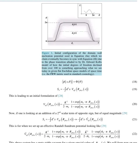
Equation (3a) after tunneling. In the potential system given as Equation (13a) we see a steadily rising scalar field value which is consistent with the physics of Figure 1. In the potential system given by Equation (13b) we see a reduction of the height of a scalar field which is consistent with the chaotic inflationary potential overshoot phenomena. We should note that φ∗ in Equation (13a) is a measure of the onset of quantum fluctuations.
Ap-pendix I is a discussion of axion potentials which we claim is part of the contribution of the potential given in
Equation (13a) Note that the tilt to the potential given in Equation (13a) is due to a quantum fluctuation. As ex-plained by Guth for quadratic potentials [7],
3 1 1 2 4 4 1 1 2 2
3 3 1
16 π 16 π
P P M
M
m m
φ∗ ≡ ⋅ ⋅ → ⋅
⋅ ⋅
(13c)
This in the context of the fluctuations having an upper bound of
60
3.1 3.1
2 πMP MP
φ > ≈ ≡
⋅
(13d)
Here, φ φ> C. Also, the fluctuations Guth had in mind were modeled via [32]
12 π
m t G
φ φ≡ − ⋅ ⋅ ⋅
(13e)
3. Brief Sketch of Randall Sundrum Effective Potential and Its Links to Equation
(13a) and Equation (13b)
The consequences of the fifth dimension mentioned in Equation (10) above show up in a simple warped com-pactification involving two branes, i.e. a Planck world brane, and an IR brane [28]. The IR brane can be thought of as similar to a Casmir physics plate model, parallel to the usual Universe brane, with a small separation be-tween the two branes. This construction with the physics of this 5 dimensional system allow for solving the hie-rarchy problem of particle physics, and in addition permits us to investigate the following five dimensional ac-tion integral [28].
(
)
( )
(
)
π 2
2
4 5 2
5 5 5
π
1
d d π
2 M 2
m
S x θ R φ φ K φ δ x δ x R
−
= ⋅ ⋅ ⋅ ⋅ ∂ − ⋅ − ⋅ ⋅ + − ⋅
∫
∫
(14)This integral, will lead to the following equation to solve
( )
(
)
2 2 5 2 πm K K
R R
R
µ θ
µ
δ θ δ θ
φ ∂ φ φ −
−∂ ∂ + − = ⋅ + ⋅ (15)
Here, what is called 2 5
m can be linked to Kaluza Klein “excitations” [28]via (for n > 0)
2 2 2 5 2 n n m m R
≡ + (16)
This uses [33] (assuming l is the curvature radius of AdS5)
2 3 5 P M m l
≡ (16a)
This is for a compactification scale, for 5 1
m R
, and after an ansatz of the following is used [28]:
(
5)
(
5(
)
)
exp exp π
A m R m R
φ≡ ⋅ ⋅ ⋅θ + ⋅ ⋅ −θ
(17)
Figure 1. Initial configuration of the domain wall nucleation potential used in Equation (6a) which we claim eventually becomes in sync with Equation (6b) due to the phase transition alluded to by Dr. Edward Kolbs model of how the initial degrees of freedom declined from over 100 to something approaching what we see today in given flat Euclidian space models of space time
(i.e. the FRW metric used in standard cosmology).
( )
x,( )
φ θ = Φ θ (18)
( )
(
)
4
5 d eff phys
S = −
∫
x V⋅ R x (19)This is leading to an initial formulation of [28]
( )
(
)
2(
(
( )
( )
)
)
5
5 5
1 exp π
2 1 exp π
phys eff phys
phys
m R x
K
V R x
m m R x
+ ⋅ ⋅
= ⋅
⋅ − ⋅ ⋅ (20)
Now, if one is looking at an addition of a 2nd scalar term of opposite sign, but of equal magnitude [29]
( )
(
)
(
( )
)
4 4
5 d eff phys d eff phys
S = −
∫
x V⋅ R x → −∫
x V⋅ R x (21)This is for when we set up an effective Randall-Sundrum potential looking like [29]
( )
(
)
2(
(
( )
( )
)
)
2(
(
( )
( )
)
)
5 5
5 5 5 5
1 exp π 1 exp π
2 1 exp π 2 1 exp π
phys phys
eff phys
phys phys
m R x m R x
K K
V R x
m m R x m m R x
+ ⋅ ⋅ − ⋅ ⋅
= ⋅ + ⋅
⋅ − ⋅ ⋅ ⋅ + ⋅ ⋅
(22)
This above system has a meta stable vacuum for a given special value of Rphys
( )
x We will from now on use this as a “minimum” to compare a similar action integral for the potential system given by Equation (22) above.4. How to Compare the Randall-Sundrum Effective Potential Minimum with an
Effective Potential Minimum Involving the Potential of Equation (3) Above
We are forced to consider two possible routes to the collapse of a complex potential system to the chaotic infla-tionary model promoted by Guth [7].The first such model involves a simple reduction of the axion wall potential [13] as given by, especially when
N = 1
( )
2(
)
2(
(
)
)
1 cos
a PQ PQ
V a =m ⋅ f N ⋅ − a f N (23)
( )
(
)
(
)
3.7 axion 0.1 axion 0 QCDm T ≅ ⋅m T= ⋅ Λ T (24)
i.e. to declare that the axion “mass” vanishes, and to let this drop off in value give a simple truncated version of chaotic inflationary potentials along the lines given by a transition from Equation (3a) to Equation (3b) We should note that ΛQCD is the enormous value of the cosmological constant which is 10
120
larger than what it is observed to be today [1]-[3], and for now we are side steeping the question of if or not the negative valued Ran-dall-Sundrum cosmological constant [28]
5 2
6
l
Λ = − (25)
has a bearing on this situation. Not to mention the problems inherent in several proposed fixes to the cosmolog-ical constant problem [34].
Now if we want an equivalent explanation, which may involve baryogenesis, we need to look at the compo-nent behavior of each of the terms in Equation (23) without assuming m Ta2
( )
T ε+ →∞
→ . Then, we need to re define several of the variables presented above. Now, in the typical theory presented by
( )
(
)
(
)
(
(
)
)
2
2 2
1 cos 1 cos
2
P
a PQ PQ
M
m f N a f N
φ
⋅ − ∝ ⋅ ⋅ − (26)
We then have to present a varying in magnitude value for the “scalar” φ involving ultimately the Bogol-molnyi inequality. I have done several of these for condensed matter current problems, but for our cosmology situation, we first have to work with
(
PQ)
a f N φ
≈
(27)
There has been credible work with instantons in higher dimensions, starting with Hawking’s 1999 article [31]. This, however, addresses a way of linking an instanton structure with baryogenesis, dark energy, and issues of how Randall-Sundrum brane structure can be used to formation of initial conditions of inflationary cosmology.
Clarifying what can be done with an instanton style quantum nucleation in multiple dimensions [36] may help us with more acceptable models [6] [37] as to estimating, roughly, a quantum value for the cosmological con-stant, as an improvement in recent calculations. I refer interested readers to Appendix II on this matter, but for now will restrict this discussion to a qualitative derivation done for condensed matter currents for motivational purposes only. Start with a wave functional
(
3)
(
4)
space Euclidian
exp d x dτ LE exp d x LE
Ψ ∝ −
∫
≡ −∫
⋅ (28)(
)
2{ }
(
)
2{ }
0 0 0
1 1
2 2
E Q
L ≥ Q+ ⋅ −φ φ →→ ⋅ −φ φ ⋅ (28a) where
{ }
= ⋅ ∆ ⋅2 Egap (28b) This leads, if done correctly to the quadratic sort of potential contribution as given by [37]( )
(
2)
exp
µ µ µ
ψ ϕ ≡ψ ⋅ α ϕ⋅ , At the same time it raises the question of if or not when there is a change from the 1st to the 2nd potential system,
This is for his chaotic inflation model using his potential; I call the 2nd potential
Let us now view a toy problem involving use of a S-S’ pair which we may write as [17]-[19]
(
)
(
)
π tanhb x xa tanhb xb x
φ≈ ⋅ − + − (29) This is for a di quark pair along the lines given when looking at the first potential system, which is a take off upon Zhitinisky’s color super conductor model [11].
5. Summarizing Different Approaches to Forming a Cosmological Constant
see it referred to as a “natural” cosmological constant value in terms of Planck Energy values. This is similar to the problems one observes in a Quantum Field theoretic vacuum summation of zero point energy bosonic fields up to Planck energy values [3].
4 Plank
natural ~ 3 3 observed
E
c
Λ Λ
⋅
(30a) V.G. Gurzadyan, and She-Sheng Lue wrote a world scientific paper [30]giving a derivation to the effect that one can calculate a realistic value for the cosmological constant based upon a wave number based upon a va-cuum fluctuation model which gives a Fourier style de composition of vava-cuum fluctuation wave modes such that if we assume no angular momentum “twisting” and a flat FRW metric
(
)
(
( )
)
3
2 3
d 8 π
2 π r
k
G ε k k
Λ = ⋅ ⋅ ⋅ ⋅ =
⋅
∫
(30b)Needless to say though, that any energy density so accumulated would be far, far less than what was assumed in the typical bosonic field calculation, above, especially since if ascale≡ scale factor size of the universe.
scale π
r n k
a
⋅
= (30c)
This equation would get dramatically smaller for increasing age of the universe to present conditions, with the initial values of it to be similar in “form” to the enormous values of initial energy density outlined above for an initial nucleating universe, especially if we model the initial energy as proportional to the square of Equation (30c) above. This, however, has a serious defect in that it does not give a genesis, or origins reference as to how the cosmological constant could evolve from initial big bang conditions. Mainly due to it being extremely diffi-cult to form ascale≡ scale factor size of the universe for initial conditions in the neighborhood of a cosmic
sin-gularity for times in the neighborhood of Planck’s time tP.
Part of the misconception which I think is endemic in this field with respect to forming a cosmological con-stant which is consistent with known astrophysics observations lies in the difficulty of forming of an effective Field theoretic Hamiltonian for calculation of vacuum energy, i.e. for quasi particles making sense of
vacuum vacuum 1
QFT H V
ε = ⋅ (30d)
G.E. Volovick writes a candidate for an acceptable Hamiltonian in this above equation as having a chemical potential addition [3], i.e.
chemical
ˆ ˆ
QFT
H ≡H−µ ⋅N (30e) This assumes that one can actually define a number operator for quasi particles, i.e.
3
ˆ d
N =
∫
x⋅ Ψ ⋅ Ψ∗ (30f)Again, for early universe conditions, how does one form Ψ for early states of matter? There is a huge lite-rature on this subject, which will be referred to at the end of this document [24] [25] but the wave functionals of the universe ideas, while promising in their own right for tunneling probability conditions for initial nucleation are time INDEPENDENT constructions and do not answer as to changes of initial states of matter-energy very effectively. In addition it is also important to note that initial states of cosmology are being modeled by applica-tion of topological defect, and branes very successfully [26] [27]. Still though, if Equaapplica-tion (1d) were actually defined well, we could then start to calculate a field theoretic version of Equation (1b), at least in principle, without having an undetermined at Planck time tP scale factor, as seen in early universe versions of Equation (1c). All these considerations, plus a discussion with Dr. Steinbeck at the UCLA dark matter-dark energy confe-rence in 2006 lead to a review of Abbots hypothesis.
would permit work with a satisfactory cosmological constant8 value based upon a vacuum energy expression given below(with λother being non a non axion field φ contribution to total vacuum energy) [8]
( )
total λother V φ
Λ = + (31)
As Abbot admitted though, this model, while giving certain qualitatively attractive features involved an un-acceptably long period of final tunneling time based upon [8]
( )
4 exp
M B
Γ ∝ ⋅ − (32)
with
2
N
B≈M f V (33) This idea assumes as Abbot postulated a cascading series of minimum values of V
( )
φ for a potential given by( )
4 cos2 π 2 π
N
N N
V M
f f
φ
φ ≡ + ∈ ⋅φ
⋅ ⋅ ⋅ ⋅
(34)
Equation (4) lead to a cascading series of local minimum values, where Abbot scaled the local minimum val-ues via setting his scalar field as φN =N, where N is an integer. It so happens that each minima of Equation (4) had a vacuum density value of
0
N
V = + ∈V (34a)
This assumes V0 is the vacuum energy of the minimum with the smallest given value of Equation (1g)
possible. Also, we assume that VN −VN−1= ∈.
Typical values for the constants above were 16
~ 1 eV, ~ 10 eV, ~ 0.1 eV
M f ∈ .
This lead to, for final values of tunneling time of the order of 1010120 [1]-[3] years, for a final cascade value of
( )
0
N
V ≡ φ chosen so that Λtotal≤ ∈ for a value of vacuum energy which was in sync with observed values of a
model with realistic cosmological parameters. In particular, it is useful to keep in mind that ΛQCD≤100 MeV, and that we are attempting to remove such eccentric values from our calculations. This is in line with a through going construction of a potential system which has ONE transition from a false to a true vacuum, rather than the multiple local minimums Abbot used in his washboard potential model. We expect this will lead to criteria for formation of the escape of gravitons from an early universe brane construction which evolves toward De Sitter space cosmology as a consequence of inflation. In addition we will also address how gravitons could exist, and tie in with the initial production of dark matter-dark energy, while accepting the difficulty of detecting them in post inflationary cosmology models of galaxies, and other strong gravitational centers seen in present day astrophysics.
We looked at Ariel Zhitnitsky’s formulation of how to form a condensate of a stable instanton style configu-ration of cold dark matter as a starting point for how an axion field can initiate forming a so called QCD ball [11] The QCD ball forms instanton configurations which we use to help compute an upper bound to the cosmological constant which we claim is pertinent to the release of gravitons from a brane [28].
Note that in classical GR, potential diagrams have proved useful in analyzing orbits of particles and photons in Schwartzschild geometry. Here, we use the di quark model so formed here as to add in a physically realistic upper bound to forming a cosmological constant input into analyzing when gravitons could be released from an early universe brane. This is similar in part to the use of potential diagrams in investigating Lorentz violations in
5
AdSS bulk background [29], and we are extending the same methodology to brane motion and graviton mo-tion in AdS5 and AdSS5. We also add that our method is useful since it is a bridge from a metric with dS≅0
in the case of initial nucleation of di quark pairs to the more standard dS≠0 in standard Schwartzshield geo-metry, while assuming our branes form in dS≠0.
the potential at the start of di quark nucleation of the scalar field itself. This will be elaborated upon in the con-clusion of this document and will constitute part of a follow up of the ideas of this document for future research inquiry. This happens in spite of a transition from a tilted washboard potential to a potential materially similar to Guths quadratic chaotic inflationary potential [7].
We also claim that the process of forming instantons as spoken of in the formation of di quark pairs in itself is useful for the later formation of cold dark matter in the form of QCD (Quantum Chromodynamics) balls, as is elucidated upon later in this document. In addition is the datum that the main part of the potential for forming the single tunneling washboard potential used in the formation of di quark pairs is extremely similar to a cosmic axion potential which is known to have a temperature dependence. This axion potential, as is stated in one of the appendix entries disappears as temperature increases, leading to the more typical Guth chaotic inflationary po-tential [7] which is then used as a template to fine tune the fluctuation of scalar popo-tential values toward the end of the cosmic inflationary period [7]. We assert that this period of transformation would lead to extensive gravi-ton production in an early universe, as well as dark matter production in a way which is observable via the pro-posed JDEM satellite system.
7. Introduction of Spalerons for the Early Universe as a Generalization of
Cosmological Instantons for a Re Do of Abbots Procedure
As referred to in Mukhanov’s book on foundations of cosmology, spalerons are a way to introduce motion of a “quasi particle” in a Euclidian metric via use of Wick rotations τ = −it Mukhanov introduces two ways for an instanton (spaleron) to have an escape velocity from a rotated Euclidian metric defined potential, in terms of a given thermal bath of temperature T. The two limiting cases are in part defined by the formation of an instanton action SI, with [14]
( )
Rate of escape determined by the instanton
m I V q T
S ⇒
(35a)
This assumes
( )
EV q (35ai)
Next
( )
Period of oscillation is about zero
m
I V q T
S ⇒
(35b)
This assumes
( )
E≈V q (35bi)
When we have the energy of the system close to Equation (35bi), we are in the realm of a first order approxi-mation of escape probability of constituents of a scalar field φ given by
sphalerons exp E
P
T
∝ −
(35c)
This assumes that the energy (mass) of a sphaleron is defined via
( )
sphalerons m
E ≈V q (36)
primary contribution to cosmological initial conditions we can measure
8. Zhnitinisky’s QCD Balls, and Their Contribution to Cosmological Instantons
We looked at Zhitnitsky’s formulation of how to form a baryon condensate to initiate forming a so called QCD ball [11]. This QCD ball could in fact be the template for the initial expansion of a scalar field leading to false vacuum inflationary dynamics in the expansion of the universe. Zhitnitsky’s formulation uses quarks in a non-hadronic state of matter, but which in the beginning can be in di quark pairs. In doing so, Zhitnitsky’s cal-culations for quarks being squeezed by a so called QCD phase transition due to the violent collapse of an axion domain wall should be used. The axion domain wall would be the squeezer to obtain a soliton (anti soliton) figuration. This pre supposes that we are using a multiple dimensional generalization of the baryon number con-tribution8 9
B
M ≈B (37a)
And, Zhitnitsky [11] further gives a criteria for absolute stability by writing a region of stability for the QCD balls dependent upon the inequality occurring for B>BC (a critical charge value)
B N
M m
B
∂ >
∂ (38)
He furthermore states that stability, albeit not absolute stability is still guaranteed with
1B<BC (39)
This is done in such a manner as to use Figure 1 as a condensed matter physics template which is analogous to the instanton behavior of di quark pairs. Furthermore I also claim that it gives a reason for the inclusion of axion physics as seen in the first part of Equation (6a) with respect to the axion walls alluded to in Appendix II
below. We should note though that Kolb’s “The Early Universe” book [13] also gives a temperature dependence of axions which is of the form of
( )
(
)
(
)
3.7axion 0.1 axion 0 QCD
m T ≅ ⋅m T= ⋅ Λ T (40)
It is important to note that Abbots potential [8] as given above has multiple cascading false vacuum minimum. We are assuming just one minimum, with a final value as given for the first potential system above. Also, if the initial tunneling system is started off with the value of the exponent of Equation (32)
2 2
1
N
B ≈M f V →M V (40a)
Then I claim that the tunneling problem Abbot spoke of can be scaled out as to obtain tunneling times not in-congruent with respect to a reasonable age of the universe.
We should note that ΛQCD is the enormous value of the cosmological constant which is 10
120
larger than what it is observed to be today. However, if axions are involved in the formation of instanton physics for early universe nucleation, then Equation (40) tells us that as can be expected for very high initial temperatures that axions are without mass but exist as an energy construct, which is not so surprising
Why in this model did I work with a 2nd potential system as well? The reason is because that the first potential system in its emergent fashion is congruent only with the first slow roll condition assumed as necessary for in-flation, i.e. if we look at
2 , 120
10 V 1
V
φ
(41)
We find that V1 fits this requirement for small φ values, but is inconsistent with respect to the following
formulation given in Equation (42) below.
, 1
V V
φφ
However, if we work with V2 that both of these conditions would be amply satisfied. The trick though is to
obtain a value of Equation (40) which is not so small as to get the problems Abbot [8] obtained in the mid 1980s which lead to his bound being abandoned due to the effectively infinite time expected in tunneling from a false vacuum minimum to a closer to the general true potential minimum [1] [2].
9. Estimation of Tunneling Time for New Potential System Given in Equation (13a)
and Equation (13b)
An easy, straightforward manner to calculate tunneling time in the case of a false vacuum is to use a WKB type bounce calculation for forming an energy based tunneling [31]
( )
tunneling
WKB
S E
E
τ ≈ ∂ ⋅
∂ (42a)
We need now to do this for a potential system given in part by Equation (5) above, and to do it consistently. Assuming that SWKB
( )
E ≈SI( )
E via a Coleman thin wall approximation for a bubble of space time, this leads to [14] [31]( )
2 3 427 π 2
I
S E
E
σ ⋅ ⋅ ≈
⋅
(42b)
Here, σ is the surface tension of a bubble, and
min
E≡V (42c)
If one defines the minimum of the potential as being due to the 1st tilted washboard potential E≡Vmin is not
going to be a zero quantity, and we will have a non zero but not huge value for tunneling time. This explicitly uses [14]
( )
crit 3
V
R σ
φ∗ ≈− ⋅ (42d)
If Rcrit∝lP, i.e. is on the order of Planck length, and V
( )
φ Vmin∗ ∝
of the 1st tilted washboard potential given in Equation (13a), this construction leads to a non zero, but not enormous tunneling time for instantons in the bubble of space time used for an early universe configuration, this will lead to [8]
critical
totalR λother Vmin observed
Λ = + ≈ Λ (42e)
This explicitly assumes that one is using the tilted washboard potential of Equation (13a)
10. Necessary Conditions for Axion Wall Potential Contribution to Equation (13a)
Disappearing
What suffices to initiate chaotic inflation? Note that a potential
( )
1 nV ≈ n ⋅φ (43) Involves a change of scale factor of the form [14]
( )
(
)
4 π(
2 2( )
)
exp
init init
a t a t
n
φ ≅ ⋅ ⋅ ⋅ φ −φ
(44)
As the mass of Equation (40) largely disappeared, this would be in tandem with higher powers of n disappearing, leading to
( )
( )
2AXION 0
1 n 1 2
V ≈ n ⋅φ →→ ⋅φ (44a) This would be in tandem with [14]
( )
(
2 2)
(
2 2( )
)
AXION 0
4 π 4 π
exp exp
2
init init init init
a t a t
n φ φ → φ φ
⋅ ⋅
⋅ ⋅ − → ⋅ ⋅ −
(44b)
11. Using Our Bound to the Cosmological Constant to Obtain a Conditional Escape
of Gravitons from an Early Universe Brane
In forming this problem, we offer an initial review of the basic physics we are assuming leads up to this problem. The physics shown in Equation (13a) to Equation (13b) above, corresponds to a phase transformation from
0
dS≅ in the case of initial nucleation of di quark pairs to the more standard dS≠0 expected in the mists of to aftermath of inflation. This is where we will use the bound to a cosmological constant given in Equation (40) to determine how we can, address the question of what would be a necessary condition for gravitons to leave an early universe brane, and also to address if they leave an early universe brane, why it is generally going to be extraordinarily difficult to detect gravitons in post inflationary cosmological astrophysical structures [16], such as galaxies. In a nutshell, we believe that the formation of early universe structures at the conclusion of inflation ended the generation of most gravitons, and that it will necessitate a different search methodology in order to obtain graviton signatures experimentally.
Our discussion in part is a brief introduction to the. brane structure built by Leach, and Lesame in their article about escape of gravitons from a brane [46]. It is noticeable that their contribution makes use of an effective po-tential for gravitons which includes cases where the brane would conceivably move at the same speed as escap-ing gravitons, and the more desirable case that gravitons moved faster than the brane itself, and escaped to propagate through inter galactic space in the way we see today. Our use of di quarks would be for an emergent structure filling in the bridge between the 1st and 2nd potentials of Equation (5) above, and our analysis of the eventual bound to the cosmological constant is commensurate with an early universe producing most of gravi-tons we would expect in our present universe. Our candidate for graviton production would be when we are producing cold dark matter in the form of QCD balls as written up by Zhitinisky in his model of QCD color su-per conductors as a cold dark matter candidate [11]. We also believe that we are tying in this initial su-period of graviton production with cold dark matter, and that further analysis will lead to refining how to effectively search for gravitons. i.e. the place to start would be in early universe objects, perhaps like quasars.
To begin we present using the paper written by Leach et al. on conditions from a FRW brane [28] in early universe cosmology, assuming that the cosmological constant input is formed as a result of the immediate con-sequences of the phase transition indicated in Equation (13) above. This also assumes that what we call the cosmological constant was likely initially greater than the final value given for inflationary potentials of the 2nd type given in Equation (13b).
We are assuming explicitly that we can use a Friedmann-Lemaître-Robertson-Walker brane world at or near the end of inflation, and that it is embedded in a structure similar to a 5-dimensional anti-de Sitter Schwartzshield bulk [28]. Why are we doing this? Frankly to utilize the effective graviton potential argument built up by J. Leach et al. as to how a cosmological constant plays into would be release of gravitons from a brane. I believe this criteria is unique, and deserves further analysis.
We shall briefly summarize their findings and put in our work on di quark contributions to an upper bound to the cosmological constant as an enabler of graviton production from this brane structure. A further unstated as-sumption is that the gravitons were likely released in a brief instant after di quark nucleation. This will be dis-cussed in lieu of the presumed experimental difficulties as to graviton detection via conventional detectors, with recommendations as to how to find gravitons experimentally if they are as I suspect primarily released in early universe inflationary expansion.
( )
( )
22
k
f R
B R
R
= (45)
Also there exists an “impact parameter”
2 2
2
E b
P
= (46)
This leads to, practically, a condition of “accessibility” via [28]
( )
b≥B R (47)
Note, that in this definition, R so defined is with respect to “bulk dimensions” and from considerations of a five dimensional anti de Sitter Schwartzshield metric
( )
22 2k
R
f R k
l R
µ
= + − (48)
Here, k = 0 for flat space, k = −1 for hyperbolic three space, and k = 1 for a three sphere, while we also set an anti-de Sitter radius of curvature [28]
6
l≡ −
Λ (49)
This assumes a negative bulk cosmological constant Λ and that µ is a five dimensional Schwartzshield mass. In addition we also should note that if we assume that the initial configuration of our universe was indis-tinguishable from a giant black hole and that there exists an effective “radius” for emission of a graviton from a bulk horizon (of super condensed matter-energy) via our standard scale factor a t
( )
( )
( )
b
R t =a t (50)
Then we have a maximum effective potential of gravitons defined via
( )
22
1 1
4
t
B R
l µ
= +
⋅ (51)
This leads to a bound with respect to release of a graviton from an anti De Sitter brane as defined by Leach et al. as
( )
tb≥B R (51a)
How do we link this to our problem with respect to di quark contributions to a cosmological constant? Here I make several claims.
Claim 1.
It is possible to re define l≡ −6
Λ as
6
eff
eff
l =
Λ (52)
Here, I am defining Λeff as being an input from Equation (1) above, with respect to a potential being defined
via a mid way transition between the 1st and the 2nd potentials of Equation (5) above. This new value for leff is
then put into a redefined values for a maximum effective gravitational potential
( )
2
2
1 1
4
eff t eff
B R
l µ
= +
⋅ (53)
Claim 2.
( )
( )
b
Planck time and in fact the entire idea of a de Sitter, let alone an anti de Sitter metric is not definable in such a physical regime.
Claim 3.
Equation (5) has a 1st potential which tends to be for a di quark nucleation procedure which just before a de-fined Planck’s time tP permits input into the formation of a cosmological constant according to Equation (40). But that the cosmological constant was prior to time tP likely far higher, perhaps in between the values of the observed cosmological constant of today, and the QCD tabulated cosmological constant which was/is 10120 time greater. i.e. that there was in fact for the region in between the 1st and the 2nd potential systems of. Equation (5)
( )
2 2
2
1 1
4
eff t eff
b B R
l µ
≥ = +
⋅ (54)
With furthermore
2 2
1 1
P P
eff t t eff t t
l l
< ≡
(55)
So then that there would be a great release of gravitons at or about time tP.
Claim 4.
Few gravitons would be produced significantly after time tP. So it would be imperative for researchers to look at early universe objects such as quasars, etc. in order to obtain events consistent with graviton production. We refer to the reader to Appendix V, which summarizes what can be said about gravitons, and early universe physics, with an eye toward distinguishing between different cosmological models.
Before we reach our conclusion, we should note that negative bulk cosmological constant used in brane world with the sort of metric referred to above assumes that there exist positive and negative tensions ±T with a ten-sion usually given by T becoming Teff in the revision which was presented as a cosmological bound
2 2
3 3
4 π 4 π
P P
eff
eff
M M
T T
l l
= → =
⋅ ⋅ ⋅ ⋅
(55a)
Still though this assumes as in Randall-Sundrum brane-worlds that the negative tension brane world has the standard model fields in the negative tension brane [5]. Also that one is able to use a finite distance between the branes to get a discrete KK spectrum, and that a distance between the branes is fixed, to recover standard GR four dimensional space time for low energy systems, which are assumed to be dominant after di quark nuclea-tion.
12. Connection to Investigating a Tie in of a Brane World Least Action Integral
with a Di Quark Least Action Integral
Now for the question the paper is raising, Can we realistically state the following for initial conditions of a nuc-leating universe? If so, then what are the consequences?
( )
(
)
(
) (
)
4 3 4
5 d eff phys d spaced Euclidian E d E
S = −
∫
x V⋅ R x ∝ −∫
x τ L ≡ −∫
x L⋅ (56)The right hand side of Equation (20) can be stated as having
(
)
2{ }
0 1 2E
L ≥ ⋅ φ φ− ⋅ . (57) We can insist that this ∆Egap between a false and a true vacuum minimum [21], that
{ }
≡ ⋅ ∆2 Egap (58)in-stanton physics and the Bogolmyi inequality [22], in order to perhaps take into account Baryogenesis? Also, can this shed light upon the Wheeler De Witt equations [13] [33] modification by Ashtekar [47] in early universe quantum bounce conditions?
Finally, does this process of baryogenesis, if it occurs lend then to the regime where there is a bridge between classical applications of the Wheeler De Witt equation to the quantum bounce condition raised by Ashtekar [24]?
13. Tie in with Di Quark Potential Systems, and the Classical Wheeler De-Witt
Equation
Ashtekar’s quantum bounce [47] gives a discretized version of the Wheeler De Witt equation. Let us first review classical De Witt theory which incidentally ties in with inflationary n = 2 scalar potential field cosmology. This will be useful in analyzing consequences of the wave functional so formed in Equation (18) and suggest quan-tum bounce analogies we will comment upon later.
In the common versions of Wheeler De Witt theory a potential system using a scale radius R t
( )
, with R0as a classical turning point value [13] [33]
( )
3 0 2 2 40 0
3 π
2
c R R R
U R
G R R
⋅ ⋅ ⋅
= ⋅ −
⋅
(59)
Here we have that if lP is a Planck length
36
0 0
3
~ P ~ 7.44 10 meters
R c t⋅ ≡l ≡ ⋅c × −
Λ (60a)
As well as
44 3
~ 2.48 10 sec
P
t −
≡ ×
Λ (61)
Now, Henriques [32] presents a way in which one can obtain a Wheeler De Witt equation based upon
( )
1(
2 2 2)
( )
ˆ
2
H⋅ Ψ φ = ⋅ Aµ⋅pφ +Bµ⋅m ⋅φ ⋅ Ψ φ
(62)
Using a momentum operator as give by
ˆ
pι i
φ
∂ = − ⋅ ⋅
∂ ⋅
(63)
This is assuming a real scalar field φ as well as a “scalar mass m” based upon a derivation originally given by Thieumann [48]. The above equation as given by Theumann [48], and secondarily by Henriques [32] lead directly to considering the real scalar field φ as leading to a prototype wave functional for the φ2
potential term as given by
( )
(
2)
exp
µ µ µ
ψ φ ≡ψ ⋅ α φ⋅ (64) As well as an energy term
Eµ = Aµ⋅Bµ ⋅ ⋅m (64a)
B A m
µ µ µ
α = ⋅ ⋅ (64b) This is for a “cosmic” Schrodinger equation as given by
( )
( )
ˆThis has
(
0 0)
6
1 2 1 2
9 4
9
p
p m
A V V
l
µ µ µ+ µ µ−
⋅
= ⋅ −
⋅ (64d)
And
( )
3
p
p m
B V
l
µ = ⋅ µ (64e)
Here Vµ is the eigenvalue of a so called volume operator, and the interested readers are urged to consult with the cited paper [48] to go into the details of this, while at the time noting mP is for Planck mass, and lP is for Planck length, and keep in mid that the main point made above, is that a potential operator based upon a qua-dratic term leads to a Gaussian wave functional with an exponential similarly dependent upon a quaqua-dratic φ2
exponent. We do approximate solitons via the evolution of Equation (64) and Equation (64c) above, and so how we reconcile higher order potential terms in this approximation of wave functional is extremely important.
Now Ashtekar in his longer arXIV article [47] make reference to a revision of this momentum operation along the lines of basis vectors µ by
2 8 π ˆ
6
P l
pι µ = ⋅ ⋅ ⋅γ ⋅µ µ (65)
With the advent of this re definition of momentum we are seeing what Ashtekar works with as a sympletic structure with a revision of the differential equation assumed in Wheeler-De Witt theory to a form characterized by [47]
2 2
φ
∂
⋅ Ψ ≡ −Θ ⋅ Ψ
∂ (65a)
Θ in this situation is such that
( )
φΘ ≠ Θ (65b)
Also, and more importantly this Θ is a difference operator, allowing for a treatment of the scalar field as an “emergent time”, or “internal time” so that one can set up a wave functional built about a Gaussian wave func-tional defined via
( )
( )
max
k k
k k ∗
≡
Ψ = Ψ (65c)
This is for a crucial “momentum” value
(
2)
16 π 3
pφ∗ = − ⋅ ⋅ ⋅G ⋅k∗ (65d)
and
0 3 16 πG ln
φ∗ = − ⋅ ⋅ µ∗ +φ
(66)
Which leads to, for an initial point in “trajectory space” given by the following relation
(
µ φ, 0)
∗ =
(initial degrees of freedom [dimensionless number] as proportional to an eigenvalue of “momentum”, initial “emergent time”)
So that if we consider eignfunctions of the De Witt (difference) operator, as contributing toward
( )
( )
1 2( )
( )
s
k k k
e µ = ⋅e µ +e −µ (66a)