Munich Personal RePEc Archive
Isolation or joining a mall? On the
location choice of competing shops
Non, Marielle
University of Groningen, the Netherlands
15 January 2010
Online at
https://mpra.ub.uni-muenchen.de/20044/
Isolation or joining a mall? On the location choice
of competing shops.
∗Marielle C. Non†
January 15, 2010
Abstract
I study the location choice of competing shops. A shop can either be isolated or join a mall. A fraction of consumers is uninformed about prices and incurs costs to travel between market places and to enter a shop. The equilibrium mall size is computed for several parameter val-ues, showing that mall and isolated shops can coexist. Several effects play a role. Mall shops attract more consumers, but isolated shops set a higher maximum price. Moreover, numerical evaluations show that an increase in mall size decreases the average price level and increases the participation level of uninformed consumers.
Keywords: location choice, travel costs, pricing, consumer search
JEL codes: D43, D83, L11, L13
∗This paper has previously circulated under the title ’Joining forces to attract
con-sumers: location choice in a consumer search model’ and is partly based on Chapter 4 of my PhD thesis. I am indebted to Maarten Janssen, Felix Munoz-Garcia, Jose Luis Moraga-Gonzalez and Marco Haan for their useful comments. The paper has also benefitted from presentations at Erasmus University Rotterdam, Tinbergen Institute Rotterdam, Univer-sity of Groningen, the EARIE 2008 meeting (Toulouse), the IIOC 2009 meeting (Boston) and the EEA 2009 meeting (Barcelona). Financial support from Marie Curie Excellence Grant MEXTCT-2006-042471 is gratefully acknowledged
†Contact:University of Groningen, WSN 763, P.O. Box 800, 9700 AV Groningen, The
1
Introduction
A city or town of reasonable size usually has multiple hairdressers, multiple grocery stores, multiple dry cleaners, and so on. Some of those hairdressers (or grocery stores, or dry cleaners, etc.) are located close to each other, for instance in a regional mall or in the city center. Others have no close competitors in their neighborhood, like a hairdresser in a small strip mall. In this paper I will use the term isolated shop for a shop that has no direct competitors nearby, whereas a shop that does have competitors nearby will be called a mall shop. Both types of shops coexist, and one might wonder how this is possible. At first sight, it seems unattractive to locate next to some direct competitors in a regional mall. On the other hand, once a regional mall with strong competition and low prices exists, how can isolated shops survive?
Most previous research only answers the question of why large malls exist, see e.g. Stahl (1982a, 1982b), Gehrig (1998) and Konishi (2005). None of these papers finds the existence of isolated shops. The intuition that these papers give revolves around the heterogeneity of goods. When goods are heterogeneous, consumers prefer to visit a mall with a large variety to increase the probability of finding a good match. This increases the volume of sales in a mall and makes it profitable to locate together. This effect of heterogeneous goods is however not the complete story. Even when goods are heterogeneous and malls are more attractive for consumers, isolated shops could survive by lowering their price. This does not occur in equilibrium because of a simplifying assumption that the aforementioned papers make: consumers can only visit one market place, independent of whether it is a mall or an isolated shop. Therefore, when a consumer decides to visit an isolated shop, he or she is stuck there and the isolated shop can ask a monopoly price. Consumers anticipate this and prefer to go to a mall, where prices are lower and the choice is greater. Consequently, isolated shops attract no consumers1 and do not exist in equilibrium.
The current paper presents a three-stage location choice model where for a large range of parameters mall and isolated shops coexist in equilibrium. In the first stage shops choose a location that will maximize their individual profits, in the second stage shops simultaneously set prices and in the last stage consumers (who only know equilibrium price distributions, not the realized prices) decide whether and where to search and buy. An important difference with previous models is that consumers can search different shops in different market places. For a fractionγof the consumers, called shoppers,
1Some of the papers mentioned above assume a spatial structure where consumers and
this search comes at no cost. Therefore these consumers search all shops and will buy at the cheapest shop. The other consumers, called non-shoppers, incur costs to search in different shops and different market places. There are costs to travel between market places (travel costs) and there are costs to enter a shop once in a market place (entering costs). This has important implications for isolated shops. First, setting a price that is higher than the expected mall price plus the entering and travel cost is not profitable, since non-shoppers who initially visited this isolated shop will not buy there. Instead they will continue to search in other shops. Isolated shops are thus forced to adjust their maximum price towards the mall prices. Next to that, there is fierce competition for the shoppers. This gives isolated shops an incentive to set even lower prices. Because of these two effects isolated shops attract a share of consumers and can survive in equilibrium.
Mall shops can also survive in equilibrium, even though I assume homoge-nous goods. Homogehomoge-nous goods lead to more competition in the mall com-pared to when goods are heterogenous, but because of the entering costs that are incurred when searching another shop in the same market place the mall shops still make a positive profit. Moreover, as will be discussed later in more detail, mall shops attract more consumers per shop than isolated shops, especially when the mall is small. This increased sales volume makes locating in a mall attractive. Thus, even in a setting where variety does not play a role a mall can exist.
consumers are indifferent between visiting a mall or isolated shop. The pricing behavior of isolated shops could be interpreted as follows. Isolated shops generally set a price above the maximum mall price, but they also regularly offer a price that is low relative to the mall prices. An isolated shop will attract non-shoppers who hope to be lucky enough to find a low price. But even if the non-shopper does not find a low price he or she will stay at the isolated shop because to continue search the non-shopper has to incur travel costs.
Another interesting result is that mall shops attract more non-shoppers than isolated shops. The intuition behind this is fairly straightforward. If isolated shops would attract many non-shoppers, they would make more profits on the maximum price in their support than on the lower prices in their support, which cannot be an equilibrium situation. Put differently, isolated shops are only willing to randomize over prices when the shoppers are relatively important for them. For mall shops, the difference between the maximum and minimum price in their support is smaller and therefore they are willing to randomize over prices even when they attract many non-shoppers. A simple consequence of the uneven distribution of non-shoppers over mall and isolated shops is that mall shops make more profits than isolated shops. Still, this does not imply that all isolated shops want to join the mall. If an isolated shop relocates and joins a mall, the mall size increases, which increases competition in the mall and decreases the expected prices in the mall. The remaining isolated shops also have to adjust their prices down-wards, and as a result the profits of both the original mall shops and the remaining isolated shops decrease when an isolated shop relocates to a mall. Whether the profits of the relocating shop increase or decrease depends on the number of consumers that are gained by relocating to the mall and on the size of the decrease in prices. As the analysis will show, in some cases it is profitable to join a mall and capture additional non-shoppers, whereas in other cases the decrease in prices is too strong to make joining a mall profitable. When the costs of visiting a shop are high, a third effect plays an important role in the location choice of shops. As in Janssen, Moraga-Gonzalez and Wildenbeest (2005), when the costs to visit a shop are high, some non-shoppers stay at home and do not buy at all. When this happens and when more shops locate in the same mall, prices tend to decrease and the participation of non-shoppers increases. Thus, when an isolated shop joins a mall it will capture a larger share of non-shoppers and the total amount of non-shoppers will increase. The joint effect on the sales of the isolated shop that relocates is so strong that it is always profitable to join a mall. So for high enough search costs all isolated shops will want to join a mall and the only possible equilibrium has no isolated shops.
First, as far as I know, Dudey (1990 and 1993) are the only papers on loca-tion choice that also assume homogenous goods. In these models, consumers can only visit one market place, but once in a mall a consumer can visit all shops in that mall at zero costs. To make sure mall prices are above zero, shops compete in quantities. Because consumers can visit only one market place, and because the largest mall has the lowest prices, all consumers visit the largest mall and isolated shops do not exist. Wolinsky (1983) is one of the few papers that assume consumers can visit more than one market place. Wolinsky however only analyzes conditions under which all shops locate in the same mall, and does not give any attention to the possibil-ity of isolated shops. The paper that comes closest to the current paper is Fischer and Harrington (1996). In their model products are heterogeneous, consumers can visit more than one market place and once in the mall all shops in the mall can be visited for free. To keep their model tractable, Fischer and Harrington however need to assume that consumers expect an infinite number of isolated shops, even though in equilibrium there is a finite number of isolated shops. In the current paper, consumers know the (finite) number of isolated shops beforehand, and act accordingly. Moreover, the current paper shows that product heterogeneity is not necessary to find an equilibrium with both mall and isolated shops.
Although not written in terms of location choice, the model of Baye and Morgan (2001) is closely related to my model. In Baye and Morgan isolated shops selling a homogenous product have the option to join a platform. Consumers can at some cost visit their local isolated shop, or they can at some entrance fee visit the platform. Once a consumer has entered the platform, he can visit all shops on the platform for free. In equilibrium, shops randomize between joining the platform and staying isolated. This result resembles the main result in my paper, but the mechanism driving this result is completely different. In the setup of Baye and Morgan the competition in the platform ensures that the probability a shop joins the platform is strictly below one, while the existence of a profit maximizing platform owner ensures that the probability a shop joins the platform is strictly above zero. Next to this, the pricing strategy of the shops and the searching strategy of consumers is completely different from the equilibrium outcome in my model.
2
The model
The model has n > 2 shops in the market that sell a homogeneous good. Production costs are linear and without loss of generality they are assumed to be zero. As mentioned in the Introduction, the model has three stages. In the first stage shops choose a location that will maximize their individual future profits. I assume that only one mall can be formed. One can think of a town that has one regional mall with ample space for new shops and several much smaller in-town mini malls that have no space to expand and accommodate new shops. A shop thus has to choose between locating in the regional mall, next to some competitors, or locating in a mini mall without any direct competitors. In the remainder of this paper I will refer to the regional mall with several competitors as the ’mall’. A mall withk∗ shops is an equilibrium when none of the mall shops can increase its profits by leaving the mall and none of the isolated shops can increase its profits by joining the mall.
In the second stage, the shops choose a price. I explicitly allow for a mixed strategy that depends on mall sizekand on whether a shop is isolated or a mall shop. Therefore the price strategy of an isolated shopj is denoted by a price distributionFkji (p), whereFkji (p) is the cdf of the price distribution. The strategy of a mall shophis denoted by a price distributionFkhm(p) The maximum price is denoted by pikj or pmkh and the minimum price bypikj or pmkh. Note that if isolated shopj(mall shoph) chooses a pure price strategy with price p∗ the price distribution is given byFi
kj(p) = 0 (Fkhm(p) = 0) for
p < p∗ and Fkji (p) = 1 (Fkhm(p) = 1) for p≥p∗. In the next sections it will however become clear that there is no symmetric pure strategy equilibrium. In the third stage of the model consumers decide on whether and where to search and buy. The model has a unit mass of consumers, all having unit demand and a valuationθ for the product. The consumers are aware of all the locations of the shops, but they do not know the prices in the shops. They however form rational price expectations and base their decisions on these expectations.
There are two different types of consumers. A fractionγ of consumers con-sists of shoppers who have zero entering and travel costs. As a consequence shoppers know all the prices and buy at the cheapest shop.2 A fraction
2One could think of shoppers as consumers who obtain a strictly positive utility from
1−γ of consumers consists of consumers who incur strictly positive entering and travel costs. These consumers are referred to as non-shoppers. Non-shoppers incur entering costs ce > 0 when entering a shop. These costs
are incurred whenever a not previously visited shop is entered and do not depend on whether a shop is in a mall with several shops or is an isolated shop. The entering costs are equivalent to the continuation costs in a stan-dard consumer search model. These costs reflect the time spent in the shop, finding the product on the shelf, finding the price of the product, waiting for a shop assistant to help you, etc. Note that positive entering costs are essential in the model. Without entering costs non-shoppers could without additional costs search all the shops in the mall. This would drive the mall prices to zero, and no shop would ever locate in a mall. In addition to the entering costs, non-shoppers incur travel costsct >0 whenever they travel
from their house to a market place or travel between market places, where a market place can be either a shopping mall with several shops selling the product or an isolated shop. The travel costs are incurred every time a non-shopper travels between market places, and therefore are also incurred when returning to a previously visited shop that is in a different market place than the market place where the non-shopper currently is.3 The travel costs can
be interpreted as the costs of, say, a bus ticket or petrol costs. The travel costs ensure that searchinghshops in the same mall comes at less costs than searchingh shops spread over different market places. Finally, the analysis is restricted to values ofce andctfor which ct+ce< θ.
Non-shoppers search sequentially. This means that non-shoppers first decide on whether to stay at home, visit a mall shop or visit an isolated shop. Let µk denote the fraction of non-shoppers who decide to visit a shop (active
non-shoppers) when the mall has size k and let 1−µk denote the fraction
of non-shoppers who decide to stay at home. The fractionµk is determined
in equilibrium. Based on the price found in the first shop, an active non-shopper decides on whether to search a second shop and whether this second search will be in the same market place as the first search (if possible) or in another market place. Then, based on the outcome of the second search, active non-shoppers decide on whether or not to search a third time and where the third search will be, etc.
In the analysis below I will derive a subgame perfect equilibrium of the three
the presence of a fraction of consumers with zero entering and travel costs.
3These return costs are necessary to prevent arbitrage. Imagine a situation of one
stage game described in this section. I will focus on symmetric equilibria in the sense that all shops in the same market place choose identical price distributions and market places of the same size have identical price distri-butions as well. Note that identical price distridistri-butions do not necessarily imply identical prices because realized prices could differ from each other. Because price distributions are symmetric where possible and because I only consider situations where there is at most one shopping mall I drop the shop indicesj and h inFkji (p),Fkhm(p), pikj,pmkh,kji and pmkh. Also, fork= 1 and k=nI drop the indicesiand mbecause in those cases either all shops are isolated or all shops are in the mall.
Because shops choose symmetric pricing strategies, non-shoppers a priori have no preferences over shops that are located in the same mall. Moreover, non-shoppers a priori have no preferences over the isolated shops. Once a non-shopper has chosen to visit the mall he will therefore choose a random shop from this mall. In the same vein, once a non-shopper has decided to visit an isolated shop he will choose such a shop at random.
3
Two opposite cases:
only isolated shops and
only mall shops
Only isolated shops
This subsection gives some results on consumer behavior and pricing behav-ior of shops when all shops are isolated. In this case each visit to a shop comes at cost ct+ce, and each return visit to a previously visited shop
comes at costct. This model is equivalent to the model in Janssen,
Moraga-Gonzalez and Wildenbeest (2005) (henceforth JMW) except for the return costs, which are absent in the JMW model. It is however relatively easy to show that the equilibrium derived in JMW also holds in a model with return costs and in this section I will focus on this equilibrium.4 For the sake of
brevity many details are omitted. See JMW for a more extensive discussion.
One key component of the equilibrium is the so-called reservation price r1,
implicitly defined by
Z r1
p1
(r1−p)dF1(p) =ct+ce.
The reservation price is defined in such a way that non-shoppers will stop searching as soon as they find a price at or below r1. In JMW the unique equilibrium has p1 ≤r1 and therefore I will concentrate on an equilibrium
4Return costs complicate a full analysis considerably and could potentially lead to
with p1 ≤ r1. The derivation of the equilibrium shows that there is only
one equilibrium withp1 ≤r1, although there could also exist equilibria with
p1 > r1.
Note thatp1≤r1implies that non-shoppers will immediately stop searching
after they visited the first shop. This in turn implies that non-shoppers will only start searching when θ−Ep1−ct−ce ≥0, with Ep1 = Rpp1
1
pdF1(p).
Becausep1 ≤r1, the definition ofr1 can be rewritten asr1−Ep1 =ct+ce.
This gives that non-shoppers will only start searching when θ≥r1. When
θ > r1 all non-shoppers will search and µ1 = 1. This situation will be
referred to as ’full search’ and occurs if and only if ct+ce is below some
thresholdC∗. Whenθ=r1, non-shoppers are indifferent between searching
and not searching, and 0 < µ1 < 1. This situation will be referred to as
’partial search’ and occurs if and only if ct+ce is above C∗ and below θ.
When θ < r1, non-shoppers do not search at all. Note that in that case
shops only sell to the shoppers. This will drive the prices down to zero, and soθ < r1 can only occur whenct+ce> θ. By assumption, ct+ce< θ, and
therefore at least some non-shoppers will search in equilibrium.
Deriving the optimal pricing behavior of shops is a fairly straightforward exercise. When all shops set a price at or below r1 it is easy to see that
deviating to a higher price leads to zero profits. Also, if p1 < r1, it would
be profitable to deviate to r1, so in equilibrium p1 =r1. Setting the profit
functionπ1(p) equal toπ1(r1) gives the equilibrium price distribution. The
next Propositions summarize.
Proposition 3.1 (Full search equilibrium,µ1= 1 )
If ct+ce < θ(1−
R1
0 1+1−γγ1nyn−1dy) then all non-shoppers are active.
Non-shoppers will stop searching as soon as min(p∗, pmin+ct)≤r1, with p∗ the
price found in the shop that was last visited, pmin the lowest price found in
previously visited shops (infinite when there are no previously visited shops) and with r1 defined as
r1=
ct+ce
1−R01 1
1+1−γγnyn−1dy .
Shops randomize overp∈[1+γ1−(nγ−1)r1, r1]according to the price distribution
F1(p) = 1−(
1−γ γn
r1−p
p )
1
n−1.
Expected profits are given byπ1=r11−nγ.
Proposition 3.2 (Partial search equilibrium, 0< µ1<1)
Ifct+ce> θ(1−
R1
0 1+1−γγ1nyn−1dy)a fraction0< µ1<1of the non-shoppers
is active, whereas the remaining fraction1−µ1 of non-shoppers is inactive.
0 0.05 0.1 0.15 0.2 0.25 0.3 0.35 0.4 0.45 0
0.01 0.02 0.03 0.04 0.05 0.06 0.07 0.08 0.09
ce+ct
profits
[image:11.595.124.417.127.364.2]π1
Figure 1: Expected profits as a function of the search costs when all shops are isolated. This figure is based on 10 shops, 10 % shoppers and a valuation of the product of 1.
h(µ1)≡
Z 1
0
1 1 +(1−γnγ)µ
1y
n−1dy=
θ−ct−ce
θ .
Active non-shoppers stop searching as soon asmin(p∗, pmin+c
t)≤θ. Shops
randomize over p∈[ (1−γ)µ1
γn+(1−γ)µ1θ, θ]according to the price distribution F1(p) = 1−(
(1−γ)µ1
γn
θ−p
p )
1
n−1.
Expected profits are given byπ1=θµ11−nγ.
Figure 1 shows the expected profits as a function of the search costsct+ce.
In this figure, the number of firmsnequals 10,γ = 0.1 andθ= 1. With these parameter values the full search equilibrium holds forct+ce<0.073 and the
partial search equilibrium holds for 0.073< ct+ce<1. Note that a search
cost value of 0.073 implies that the search costs are 7.3% of the valuation of the product. The expected profits are plotted forct+ce <0.45; for higher
values ofct+cethe profits are decreasing and whenct+ceapproaches 1 the
[image:11.595.193.406.448.480.2]Only mall shops
When all the shops are in the same mall non-shoppers incur costsce+ctfor
the first search, they incur costscefor every next search and have no return
costs. This model is equivalent to JMW except for the fact that the first search is more costly than every next search. There is a unique equilibrium, and once a non-shopper has visited one shop, the analysis is the same as in JMW. More specific, non-shoppers will stop searching as soon as they find a price at or below the reservation pricern, which is defined by
Z rn
p
n
(rn−p)dFn(p) =ce.
Note that the righthand side of this expression isce, instead of ce+ct for
the definition ofr1. As in JMW, the unique equilibrium haspn=rn.
The analysis differs from JMW when it comes to full and partial search equilibria. All non-shoppers will search when θ−Epn−ct−ce > 0. The
definition ofrn gives rn−Epn =ce and so all non-shoppers will be active
when rn < θ−ct. A partial search equilibrium occurs when rn = θ−ct.
Note that the travel costs explicitly occur in this expression. This is because non-shoppers incur travel costs when they search for the first time, whereas the expected prices (rn−ce) are based on their behavior once they are in
the mall, where travel costs do not play a role anymore.
Note that the maximum price that shops can ask is limited toθ−ct.
Intu-itively, the maximum price a shop can ask is limited to the expected price plus ce. For a higher price, non-shoppers would continue searching and
the shop setting the maximum price would not sell anything. On the other hand, the expected price can at most beθ−ct−ce, otherwise no non-shopper
would be active. Combined, this gives that the maximum price can at most beθ−ct.
The full search equilibrium has the following form.
Proposition 3.3 (Full search equilibrium,µn= 1)
If ce <(1−
R1
0 1+1−γγ1nyn−1dy)(θ−ct) all shoppers are active and
non-shoppers will stop searching as soon as they find a price at or belowrn, with
rn defined as
rn=
ce
1−R01 1
1+1−γγnyn−1dy .
Shops randomize over [(1−1γ−)+γγnrn, rn]according to the price distribution
Fn(p) = 1−(
(rn−p)(1−γ)
nγp )
1
n−1.
The partial search equilibrium is as follows.
Proposition 3.4 (Partial search equilibrium, 0< µn<1)
If ce>(1−
R1
0 1+1−γγ1nyn−1dy)(θ−ct) a fraction 0< µn<1 of non-shoppers
is active, where µn is defined by
h(µn)≡
Z 1
0
1 1 +(1−γnγ)µ
ny
n−1dy=
θ−ct−ce
θ−ct
.
Active non-shoppers will stop searching as soon as they find a price at or belowθ−ct. Shops randomize over[(θ−ct)γnµ+nµ(1n−(1γ−)γ), θ−ct] according to
price distribution
Fn(p) = 1−(
(θ−ct−p)(1−γ)µn
nγp )
1
n−1.
Expected profits areπn= (θ−ct)µn(1n−γ).
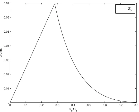
Figure 2 shows the expected profits as a function of the search costsct+ce.
Recall that the reservation valuern depends only on the continuation costs
of search,ce. Moreover, the decision whether or not to search depends onct.
Therefore, the expected profits do not depend on total costsce+ct, but on
ctand cein isolation. To be able to make a plot of the expected profits as a
function of the total costsce+ct I assume thatceand ctare related to each
other in a fixed proportion, that is,ct=β(ct+ce) andce= (1−β)(ct+ce),
or consequently ct= 1−ββce. In the figure,β = 0.8. As before, the number
of firms n equals 10, γ = 0.1 and θ = 1. The expected profits are plotted forct+ce <0.8. For higher values ofct+ce the expected profits decrease
to 0. The figure shows the same pattern as in the case where all the shops are isolated.
Comparing the two opposite cases
A comparison of the equilibria in the previous two subsections gives some new and interesting results. It can be shown that for low values of ct+ce
it is more profitable to have all shops isolated, whereas for high values of ct+ce having all shops in the same mall leads to more profits. There are
two opposing effects playing a role here. First, prices are higher when all shops are isolated. Second, more non-shoppers are active when all shops are in the same mall. When ct+ce is low the second effect is either absent or
small, but whenct+ce is high, the second effect is stronger than the first.
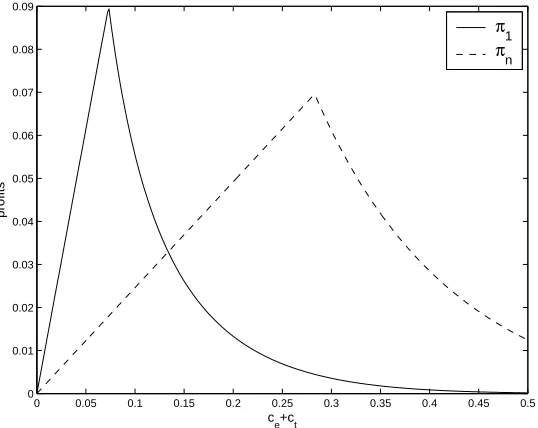
Figure 3 combines figures 1 and 2 by showing the expected profits as a function of the search costs ct+ce in the case where all shops are isolated
0 0.1 0.2 0.3 0.4 0.5 0.6 0.7 0.8 0
0.01 0.02 0.03 0.04 0.05 0.06 0.07
ce+ct
profits
[image:14.595.122.392.126.344.2]πn
Figure 2: Expected profits as a function of the search costs when all shops are located in the same shopping mall. This figure is based on 10 shops, 10 % shoppers and a valuation of the product of 1. The travel costsct are set
at 80% of the total search costsct+ce
ct= 0.8(ct+ce) and ce = 0.2(ct+ce). The expected profits are plotted for
ct+ce<0.5.
The figure can be split in different parts. First, when the search costsct+ce
are small enough (for the current parameter valuesct+ce<0.073) the full
search equilibrium holds in both cases andπ1 > πn. The intuition for this
result is straightforward. By locating together in a single shopping mall shops decrease the costs to continue search from ce +ct to ce, leading to
stronger competition and lower prices and profits. Second, when the search costs ct+ce have an intermediate value (for the current parameter values
0.073< ct+ce<0.28) the full search equilibrium holds in the case where all
shops are located together and the partial search equilibrium holds in the case where all shops are isolated. The intuition for this is as before: when all shops are located together consumers expect lower prices and therefore consumers are more willing to search. This implies that when all shops are located together all non-shoppers are active and the expected profits increase in the search costs ct+ce. When all shops are isolated however
only a fraction of the non-shoppers is active and expected profits decrease in the search costsct+ce. When the search costs ct+ce are high enough
0 0.05 0.1 0.15 0.2 0.25 0.3 0.35 0.4 0.45 0.5 0
0.01 0.02 0.03 0.04 0.05 0.06 0.07 0.08 0.09
ce+ct
profits
[image:15.595.123.392.129.343.2]π1 πn
Figure 3: Expected profits as a function of the search costs when all shops are isolated and when all shops are located in the same shopping mall. This figure is based on 10 shops, 10 % shoppers and a valuation of the product of 1. The travel costsct are set at 80% of the total search costsct+ce
equilibrium holds in both cases. The fraction of active consumers is however higher when all firms are located together and this leads to higher expected profits when all firms are located together.
The pattern shown in Figure 3 does not depend on the specific parameter values chosen. Name the value ofct+ce where the full search equilibrium
changes into a partial search equilibrium the inflection value. A close look at Propositions 3.1 and 3.3 shows that the inflection value is always higher when all shops are located together. It is also easy to see that when in both cases a full search equilibrium holds, that is, when the search costsct+ceare
below the inflection value for the case when all shops are isolated,π1 > πn.
With somewhat more effort it can be shown that πn > π1 when in both
cases a partial search equilibrium holds, that is, whenct+ce is at or above
the inflection value for the case when all shops are located together. This gives Proposition 3.5.
Proposition 3.5 Let ct= β(ct+ce) with 0 < β <1. Then there exists a
numbercsuch that for ct+ce < c π1> πn and forct+ce> c π1< πn, with
θ(1−
Z 1
0
1
1 +1−γγnyn−1dy)< c < θ
1−R01 1
1+1−γγnyn−1dy 1−βR01 1+ γ1
1−γnyn−1
4
The intermediate case
In this section I will investigate the situation where 2 ≤ k ≤ n−1 shops
are located together in a shopping mall and the remaining n−k shops
are isolated. Recall thatFkm(p) is the price distribution used by the shops that are in a shopping mall with k shops, with fkm(p) the corresponding probability density function. The support of Fkm(p) is defined by all prices for whichfkm(p)>0. Denote byπkm the expected profits of such a shop and definerkm as
Z rkm
pm k
(rmk −p)dFkm(p) =ce. (1)
The same can be defined for the isolated shops: Fki(p) is the price distri-bution used by them when k shops are located in the mall, with fki(p) the corresponding pdf. The support of Fki(p) is defined by all prices for which fki(p)>0,πik denotes the expected profits andrik is defined as
Z rik
pi k
(rki −p)dFki(p) =ce+ct. (2)
Note that the definition of rkm uses ce whereas the definition of rik uses
ct+ce. The reason for this is that a non-shopper who is in an isolated shop
and wants to continue search has to incur a search cost ce+ct, whereas a
non-shopper who is in a mall can continue searching in the mall at costce.
As before, the reservation prices determine whether a consumer wants to continue search and moreover determine whether a full search or a partial search equilibrium holds. As in the previous section, I will concentrate on equilibria wherepm
k ≤rmk and pik≤rik.
Let xk denote the total fraction of active non-shoppers who decide to first
visit a mall shop and let 1−xk be the total fraction of active non-shoppers
who first visit an isolated shop, with 0< xk <1. This implies that initially
each mall shop attracts xk
k active non-shoppers, whereas each isolated shop
initially attracts 1−xk
n−k active non-shoppers. Note that if xk = k
n the active
non-shoppers initially spread randomly over mall and isolated shops. It will be shown later that in equilibrium xk
k > k n.
complete specification of consumer behavior is therefore placed in Appendix B.
The optimal consumer behavior implies that Epik = Epmk, with Epmk the expected mall price, andEpi
k the expected price in an isolated shop.
Intu-itively, ifEpik < Epmk all active non-shoppers prefer to search in an isolated shop and mall shops only attract shoppers. Because the number of mall shops, k, is at or above 2, this drives the prices in the mall shops down to zero and Epik < Epmk cannot hold. When there are at least two isolated shops (k ≤ n−2), the reverse argument holds for Epmk < Epik, showing that in equilibrium Epmk = Epik and non-shoppers are indifferent between first searching a mall shop and first searching an isolated shop. This also holds when there is only one isolated shop (k=n−1), but the argument is less intuitive. Appendix A provides more details. Note that whenpmk ≤rkm and pik≤rik definitions (1) and (2) can be rewritten asrmk =Epmk +ce and
rki =Epik+ct+ce. This gives the following Proposition.
Proposition 4.1 rki =rmk +ct in any equilibrium with pmk ≤rkm and pik ≤
ri k.
Recall that we concentrate on equilibria with pmk ≤ rmk and pik ≤ rki. The specification of optimal consumer behavior in Appendix B shows that when pm
k ≤ rmk and pik ≤ rik all active non-shoppers will search only once. If a
non-shopper would find a mall price above rkm or an isolated price above rki he or she would continue searching. Moreover, all non-shoppers will be active (µk = 1) when rki < θ and only a fraction of non-shoppers will be
active (µk<1) whenrki =θ. Note that if all shops setpkm≤rkmandpik≤rki,
deviating to a higher price is not profitable. A deviating shop will not sell to any shoppers and all the active non-shoppers that it initially attracts will continue searching. Therefore, a deviating shop will have zero profits. For p≤rkm the profit function of mall shops is
πkm(p) =γp(1−Fkm(p))k−1(1−Fki(p))n−k+ (1−γ)µk
xk
k p. Forp≤rik the profit function of isolated shops is
πik(p) =γp(1−Fkm(p))k(1−Fki(p))n−k−1+ (1−γ)µk
1−xk
n−kp. Assume for the moment that k < n−1. The profit functions show that in equilibrium pmk = rmk, because for a lower maximum price it would be profitable to deviate tormk. Similarly, in equilibriumpik=rki.5 A standard
undercutting argument also shows that atoms in Fm
k (p) are only possible
for those prices p∗ at which Fki(p∗) = 1. Similarly, atoms in Fki(p) are only possible for those prices p∗ at which Fkm(p∗) = 1. Exactly the same
5Note that this impliespi k6=p
m
k and thereforeF
i k(p)6=F
results on maximum prices and atoms hold for k=n−1, but the proof is less intuitive and is placed in Appendix A. Equilibrium expected profits are πkm=rmk xk
kµk(1−γ) and π i k =rki
1−xk
n−kµk(1−γ).
Note that forp≥rm k
πki(p) = (1−γ)µk
1−xk
n−kp.
This shows that isolated shops will never set a price betweenrm
k andrikand
that there will be an atom atrik. Fki(p) should also have some probability mass belowrmk because else the definition ofrki as given by (2) cannot hold. This probability mass is atomless, as well asFm
k (p).
For p ≤ rmk the price distributions can be derived by setting πkm(p) = πkm and/or setting πki(p) = πik. Suppose that for allp in [p1, p2]fki(p) = 0 and
fm
k (p)>0. That is, only mall shops set prices in [p1, p2]. Thenπkm(p) =πkm
gives
Fkm(p) = 1−
µ(rm
k −p)(1−γ)µkxkk
γp(1−Fki(p1))n−k
¶k−11
. (3)
Similarly, when for allpin [p1, p2]fkm(p) = 0 andfki(p)>0 thenπki(p) =πki
gives
Fki(p) = 1−
Ã
(rik−p)(1−γ)µk1n−−xkk
γp(1−Fkm(p1))k
! 1 n−k−1
. (4)
Finally, when for allp in [p1, p2]fkm(p)>0 andfki(p)>0 thenπkm(p) =πkm
and πi
k(p) =πik jointly give
Fki(p) = 1−
Ã
(rik−p)(1−γ)µk1n−−xkk
γp
!n−11 Ã x k
k (r m k −p)
1−xk
n−k(rik−p)
!nk−1
(5)
and
Fkm(p) = 1−
Ã
(ri
k−p)(1−γ)µk
1−xk
n−k
γp
!n−11Ã1−x k
n−k(rik−p) xk
k(r m k −p)
!n−n−k−11
. (6)
The price distributions thus depend on the supports ofFkm(p) andFki(p). It can be shown that there are three types of supports.
Proposition 4.2 In any equilibrium with pm
k ≤rmk and pik≤rik, pmk =rkm
and pik =rik. Fki(p) has an atom at p = rik, fki(p) >0 for pik ≤ p ≤b and
fi
k(p) = 0 for b < p < rik, with b < rkm. There are three possibilities for the
1. fm
k (p)>0 for b≤p≤rmk and fkm(p) = 0 elsewhere.
2. fm
k (p)>0 for pik ≤p≤aand for b≤p≤rmk, with a < b. fkm(p) = 0
elsewhere.
3. fkm(p)>0 for pik≤p≤rmk and fkm(p) = 0 elsewhere. When k=n−1 only possibility 3 can hold.
Each equilibrium type has a full search variant with µk = 1 and rki < θ
and a partial search variant with 0 < µk < 1 and rik = θ. For k < n−1
this gives a total of six equilibria and for k = n−1 this gives a total of two equilibria. The conditionπik(pik) =πik(rki) gives that in all equilibrium typespik=rik (1−γ)µk
1−xk
n−k
γ+(1−γ)µk1
−xk
n−k
. In equilibrium type 1Fki(p) is given by (4) and Fkm(p) is given by (3). In equilibrium type 2 for pik≤p≤a Fkm(p) is given by (6) and Fi
k(p) is given by (5). For a < p≤ b Fki(p) is given by (4) and
forb≤p < rmk Fkm(p) is given by (3). In equilibrium type 3 for pik≤p≤b Fi
k(p) andFkm(p) are given by (5) and (6), whereas forp > b Fkm(p) is given
by (3).
The price distributions depend on rkm,rik, xk, b and possibly on µk and a.
For each equilibrium type these variables are jointly determined by a sys-tem of equations. For each equilibrium type this syssys-tem includes (1), (2), rki = rmk +ct and (for partial search equilibria) rki = θ. On top of this,
equilibrium type 1 hasFkm(b) = 0, equilibrium type 2 hasFkm(pi
k) = 0 and
Fkm(a) = Fkm(b), and equilibrium type 3 has Fkm(pik) = 0. The resulting systems of equations are too complicated to solve analytically. This implies that it is impossible to analytically derive the parameter regions in which the different equilibria hold. Also, analytical expressions for profits, our main interest, cannot be obtained. In the next sections we will therefore resort to numerical methods.
Isolated shops randomize over a low price region [pik, b] and a single high price rki. Because of the shoppers isolated shops are willing to set a price in [pik, b], but the fraction of shoppers that an isolated shop could attract should be large relative to the fraction of non-shoppers that an isolated shop attracts. This is because the difference between rki and b is at least ct. By
setting a price at or belowb an isolated shop foregoes profits of at least ct
per consumer, which should be made up by a relatively large increase in shoppers. Because the number of shoppers is fixed at γ, it should be that the number of non-shoppers per isolated shop, 1−xk
n−k, is small. This, in turn,
affects the profits of an isolated shop. It can be shown thatπki < πmk.
Proposition 4.3 In any equilibrium withpmk ≤rmk andpik≤rik, 1−xk
n−k < xk
k
5
Comparative statics
This section will give some comparative statics results on the equilibria that have been derived in the previous section, using numerical techniques. Recall that in section 3 β has been defined as a constant such thatct=β(ct+ce)
and ce = (1−β)(ct+ce). It can be shown that in all full search equilibria
for 2≤k≤n−1 the parameterxk only depends on β,γ,nand k, and not
on ct and ce. Moreover, all reservation prices and profits can be written as
ct+ce times some function ofβ, γ, n and k. The partial search equilibria
for 2≤k ≤n−1 are more complicated, in the sense thatxk depends not
only on β,γ,n andk, but also on ct+ce. Moreover, the reservation prices
and profits are nonlinear inct+ce. This implies that whenβ,γ,nandkare
fixed, the full search equilibria can be numerically calculated. To calculate the partial search equilibria,ct+ce also needs to be specified. In this
sec-tion I will therefore concentrate on the full search equilibria; partial search equilibria will be discussed in the next section.
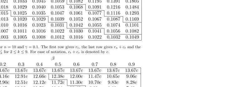
Tables 1, 2 and 3 give simulation results for the full search equilibria. Table 1 uses a small value of γ; γ = 0.05. Table 2 has an intermediate value of γ (γ = 0.1) and table 3 has a large value of γ (γ = 0.25). Each table gives results for different values ofk and β and in all tables n= 10. Each table gives a panel with results on xk
k and a panel with results on the reservation
price. For 2≤k≤n−1,ri
k is reported. Note that a full search equilibrium
only holds when rik < θ, which translates to ct+ce being small enough.
For k = 1, the tables give the equivalence of rki, r1, and the full search
equilibrium holds when r1 < θ. For k=n, the tables give rn+ct. This is
the equivalence ofrki as a full search equilibrium holds when rn+ct< θ.
Proposition 4.2 states that for 2 ≤ k ≤ n−2 three equilibrium types are possible. The simulations suggest that these equilibria do not overlap and together fill the complete parameter space. In the tables lines denote when each equilibrium type holds. The equilibria in the upper right corner, for highβ and low k, are of type 1. The equilibria in the lower left corner, for lowβ and high k, are of type 3. Note that also all equilibria withk=n−1 are of type 3. The intermediate equilibria are of type 2.
The tables suggest that xk
k increases inβ and decreases ink. To understand
this, recall that 1−xk
n−k should be such that isolated shops are indifferent
be-tween only serving non-shoppers at a pricerki and serving both non-shoppers and shoppers (with strictly positive probability) at a price in [pik, b]. When β increases, rki −rmk increases because rik−rkm = ct. This implies that it
is increasingly attractive for isolated shops to set a price rki and sell only to non-shoppers. To counterbalance this effect, 1−xk
n−k should decrease, or xk
k
(a) Values of xk
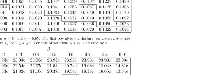
k forn= 10 andγ= 0.05.
β
0.1 0.2 0.3 0.4 0.5 0.6 0.7 0.8 0.9
2 0.1010 0.1021 0.1032 0.1044 0.1105 0.1235 0.1434 0.1776 0.2484
3 0.1009 0.1018 0.1028 0.1040 0.1052 0.1093 0.1208 0.1406 0.1826
4 0.1008 0.1016 0.1025 0.1035 0.1047 0.1059 0.1107 0.1227 0.1499
k 5 0.1006 0.1014 0.1021 0.1030 0.1041 0.1053 0.1067 0.1125 0.1305
6 0.1005 0.1011 0.1018 0.1026 0.1034 0.1045 0.1059 0.1076 0.1179
7 0.1004 0.1008 0.1014 0.1020 0.1028 0.1037 0.1049 0.1065 0.1092
8 0.1003 0.1006 0.1009 0.1014 0.1019 0.1027 0.1036 0.1050 0.1073
9 0.1001 0.1003 0.1005 0.1007 0.1010 0.1014 0.1020 0.1029 0.1044
(b) Reservation prices forn= 10 andγ = 0.05. The first row givesr1, the last row givesrn+ct and
the intermediate rows giveri
kfor 2≤k≤9. For ease of notation,ct+ceis denoted byc.
β
0.1 0.2 0.3 0.4 0.5 0.6 0.7 0.8 0.9
1 23.93c 23.93c 23.93c 23.93c 23.93c 23.93c 23.93c 23.93c 23.93c
2 23.47c 23.00c 22.54c 22.07c 21.51c 20.74c 19.68c 18.04c 14.81c
3 23.24c 22.53c 21.82c 21.10c 20.38c 19.54c 18.36c 16.65c 13.54c
4 22.99c 22.07c 21.12c 20.35c 19.17c 18.17c 17.00c 15.24c 12.26c
k 5 22.74c 21.56c 20.43c 19.22c 17.99c 16.73c 15.44c 13.79c 10.95c
6 22.48c 21.06c 19.64c 18.19c 16.83c 15.33c 13.78c 12.17c 9.62c
7 22.22c 20.57c 18.91c 17.24c 15.55c 13.87c 12.17c 10.29c 8.26c
8 21.96c 20.07c 18.19c 16.30c 14.40c 12.47c 10.49c 8.54c 6.25c
9 21.86c 19.79c 17.71c 15.62c 13.51c 11.38c 9.20c 6.96c 4.54c
[image:21.595.217.630.126.255.2]10 21.63c 19.34c 17.05c 14.76c 12.46c 10.17c 7.88c 5.59c 3.29c
Table 1: Values of xk and reservation prices for n= 10 and γ = 0.05.
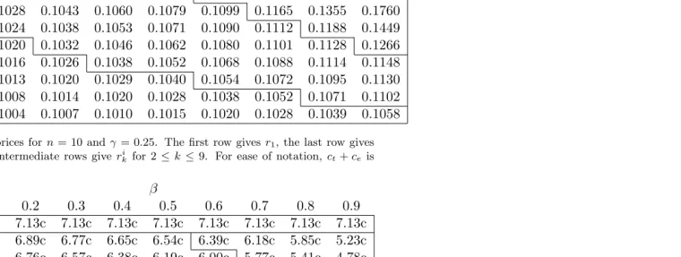
(a) Values of xk
k forn= 10 andγ= 0.1.
β
0.1 0.2 0.3 0.4 0.5 0.6 0.7 0.8 0.9
2 0.1011 0.1024 0.1036 0.1050 0.1091 0.1220 0.1416 0.1750 0.2453
3 0.1010 0.1021 0.1033 0.1045 0.1059 0.1082 0.1195 0.1391 0.1805
4 0.1009 0.1018 0.1029 0.1040 0.1053 0.1068 0.1091 0.1216 0.1484
k 5 0.1007 0.1015 0.1025 0.1035 0.1047 0.1061 0.1077 0.1116 0.1293
6 0.1006 0.1013 0.1020 0.1029 0.1039 0.1052 0.1067 0.1087 0.1169
7 0.1004 0.1010 0.1016 0.1023 0.1031 0.1042 0.1055 0.1074 0.1101
8 0.1003 0.1007 0.1011 0.1016 0.1022 0.1030 0.1041 0.1056 0.1082
9 0.1002 0.1003 0.1005 0.1008 0.1012 0.1016 0.1022 0.1032 0.1049
(b) Reservation prices forn= 10 andγ= 0.1. The first row givesr1, the last row givesrn+ctand the
intermediate rows giveri
kfor 2≤k≤9. For ease of notation,ct+ceis denoted byc.
β
0.1 0.2 0.3 0.4 0.5 0.6 0.7 0.8 0.9
1 13.67c 13.67c 13.67c 13.67c 13.67c 13.67c 13.67c 13.67c 13.67c
2 13.42c 13.16c 12.91c 12.66c 12.38c 12.00c 11.47c 10.65c 9.06c
3 13.29c 12.90c 12.51c 12.12c 11.72c 11.30c 10.70c 9.83c 8.28c
4 13.15c 12.65c 12.12c 11.59c 11.04c 10.49c 9.91c 9.00c 7.49c
k 5 13.02c 12.36c 11.73c 11.07c 10.38c 9.68c 8.97c 8.15c 6.70c
6 12.88c 12.09c 11.30c 10.50c 9.74c 8.90c 8.03c 7.13c 5.89c
7 12.73c 11.82c 10.90c 10.02c 9.08c 8.15c 7.14c 6.09c 4.96c
8 12.59c 11.59c 10.56c 9.52c 8.46c 7.38c 6.27c 5.12c 3.83c
9 12.53c 11.38c 10.23c 9.08c 7.91c 6.72c 5.52c 4.27c 2.91c
[image:22.595.216.628.117.256.2]10 12.40c 11.14c 9.87c 8.60c 7.34c 6.07c 4.80c 3.53c 2.27c
Table 2: Values of xkk and reservation prices for n= 10 and γ = 0.1.
(a) Values of xk
k forn= 10 andγ= 0.25.
β
0.1 0.2 0.3 0.4 0.5 0.6 0.7 0.8 0.9
2 0.1015 0.1031 0.1048 0.1066 0.1086 0.1183 0.1373 0.1699 0.2386
3 0.1013 0.1028 0.1043 0.1060 0.1079 0.1099 0.1165 0.1355 0.1760
4 0.1011 0.1024 0.1038 0.1053 0.1071 0.1090 0.1112 0.1188 0.1449
k 5 0.1010 0.1020 0.1032 0.1046 0.1062 0.1080 0.1101 0.1128 0.1266
6 0.1008 0.1016 0.1026 0.1038 0.1052 0.1068 0.1088 0.1114 0.1148
7 0.1006 0.1013 0.1020 0.1029 0.1040 0.1054 0.1072 0.1095 0.1130
8 0.1004 0.1008 0.1014 0.1020 0.1028 0.1038 0.1052 0.1071 0.1102
9 0.1002 0.1004 0.1007 0.1010 0.1015 0.1020 0.1028 0.1039 0.1058
(b) Reservation prices forn= 10 andγ = 0.25. The first row givesr1, the last row gives
rn+ct and the intermediate rows give rki for 2 ≤k ≤9. For ease of notation, ct+ce is
denoted byc.
β
0.1 0.2 0.3 0.4 0.5 0.6 0.7 0.8 0.9
1 7.13c 7.13c 7.13c 7.13c 7.13c 7.13c 7.13c 7.13c 7.13c
2 7.01c 6.89c 6.77c 6.65c 6.54c 6.39c 6.18c 5.85c 5.23c
3 6.95c 6.76c 6.57c 6.38c 6.19c 6.00c 5.77c 5.41c 4.78c
4 6.88c 6.63c 6.38c 6.12c 5.85c 5.58c 5.31c 4.96c 4.34c
k 5 6.81c 6.51c 6.19c 5.86c 5.53c 5.18c 4.83c 4.46c 3.89c
6 6.76c 6.38c 6.00c 5.61c 5.21c 4.80c 4.37c 3.92c 3.44c
7 6.69c 6.26c 5.82c 5.37c 4.90c 4.43c 3.93c 3.40c 2.83c
8 6.63c 6.14c 5.63c 5.13c 4.61c 4.08c 3.53c 2.94c 2.29c
9 6.58c 6.02c 5.47c 4.90c 4.33c 3.76c 3.17c 2.55c 1.88c
10 6.52c 5.90c 5.29c 4.68c 4.07c 3.45c 2.84c 2.23c 1.61c
xk
[image:23.595.215.630.109.252.2]To understand the effect ofkrecall that in equilibrium the expected isolated and the expected mall prices should be equal. The support ofFki(p) consists of [pik, b] and rik. The support of the mall prices consists of [b, rkm] and possibly some prices between pik and b. To ensure that the expected prices are equal, Fkm(p) should not attach too much probability mass to prices in [pi
k, b]. In fact, it can be shown that in equilibrium F m
k (p) < Fki(p) for p ∈
[pik, b]. Whenkincreases, an isolated shop gets less isolated competitors and more mall competitors. This increases the probability that all competitors set a price aboveband therefore increases the profitability of setting a price b. To counter this effect and make a pricerki as attractive as a priceb, 1−xk
n−k
should increase, or xk
k should decrease.
The effects ofβ and k on xk
k explain why equilibrium type 1 can only hold
for highβ and lowk. For those parameter values xk
k is high, and mall shops
have no incentive to capture all shoppers by deviating topik. On top of that, when β is high, rki −rkm is high. To ensure that expected mall and isolated prices are equal,pik should be strictly smaller thanpmk.
The tables also suggest that ri
k decreases inβ and k. To understand this,
one first needs to understand the effect of β and k on rkm. Intuitively, when k increases, the competition in the mall increases, leading to a lower reservation price rm
k . Becauserki =rkm+ct, an increase in k also decreases
rki. When β increases, ce decreases and ct increases. Equation (1) shows
thatrkm only depends on ce, and not onct. Therefore, whenβ increasesrkm
decreases. Because ri
k =rmk +ct there are two effects on rki: rkm decreases
and ct increases. The results in the tables suggest that the first effect is
stronger.
When γ increases, it seems from the tables that ri
k decreases, whereas xk
k
can both increase and decrease. When γ increases there is a stronger com-petition for the shoppers. As a result, the isolated shops are less tempted to ask pricerik and the mall shops also prefer lower prices. The tables show that indeed equilibrium type 1 occurs less often when γ is larger: the mall shops are more tempted to setpmk =pik. Because both types of shops prefer lower prices, it is no surprise thatri
k decreases. The effect on xk
k is twofold.
Isolated shops need to be indifferent between asking the high pricerik and lower prices. When the fraction of shoppers increases, isolated shops are less tempted to ask a high price, but at the same time the behavior of the mall shops leads to more competition in the lower price range, making a high price more attractive. When the first effect dominates, 1−xk
n−k needs to
increase and consequently xk
k needs to decrease to make sure that isolated
shops still want to ask ri
k. When the second effect dominates,
1−xk
n−k needs
to decrease and xk
k consequently increases to ensure that isolated shops still
want to set a low price. Note that in equilibrium type 1 the second effect is absent and that indeed xk
Even though a numerical analysis is needed to evaluate the equilibria, it is possible to analytically derive some limiting results.
Proposition 5.1 Suppose 2≤k≤n−1.
• When β→0,pi
k=p m k, r
i
k−rmk →0, Fki(p)−Fkm(p)→0 and xk →
1
n.
• When β →1, rmk →0, Fki(rmk)→1 and 1−xk
n−k →0.
• When γ →0, µk→0.
• When γ →1, pkm →0, pik→0, Fkm(p)→1 and Fki(p)→1
These results are in line with previous consumer search models, see e.g. JMW. Recall thatβdetermines the relative sizes ofctandce. Whenβ →0,
ct → 0 and in the limit consumers only incur entering costs. In that case,
the difference between mall shops and isolated shops vanishes, which leads to equal price distributions and an equal distribution of non-shoppers over the firms. Whenβ→1,ce→0. In this case, once a consumer is in the mall,
he can visit all mall shops almost for free. This leads to large competition between mall shops and consequently to prices of almost zero in the mall. To make mall and isolated shops equally attractive, isolated shops should set prices to almost zero as well. To make this possible, isolated shops should attract almost no non-shoppers. If they would attract too many non-shoppers, an isolated shop could set a pricect and make a profit on the
non-shoppers who visited the isolated shop in the first place.
When the fraction of shoppers, γ, vanishes, firms tend to focus completely on the captive consumers. This raises prices to monopoly levels, and conse-quently many non-shoppers drop out of the market. When the fraction of non-shoppers vanishes, firms compete strongly for the shoppers, leading to very low prices.
6
Location choice
In this section I will consider the equilibrium location choice of shops. A mall withk∗shops is considered an equilibrium when none of the mall shops has an incentive to leave the mall and when none of the isolated shops has an incentive to join the mall. Thus, a mall withk∗ shops is an equilibrium whenπkm∗ ≥πki∗−1andπik∗≥πkm∗+16. Note that if a mall shop would deviate
and leave the mall, the mall size would decrease by one. Also, if an isolated shop would deviate and join the mall, the mall size would increase by one.
6Rental costs that differ between locations and relocation costs could easily be
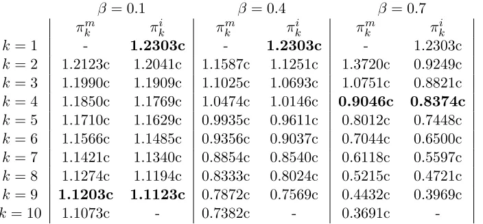
β = 0.1 β = 0.4 β = 0.7 πm
k πik πmk πik πkm πki
k= 1 - 1.2303c - 1.2303c - 1.2303c
k= 2 1.2123c 1.2041c 1.1587c 1.1251c 1.3720c 0.9249c
k= 3 1.1990c 1.1909c 1.1025c 1.0693c 1.0751c 0.8821c
k= 4 1.1850c 1.1769c 1.0474c 1.0146c 0.9046c 0.8374c
k= 5 1.1710c 1.1629c 0.9935c 0.9611c 0.8012c 0.7448c
k= 6 1.1566c 1.1485c 0.9356c 0.9037c 0.7044c 0.6500c
k= 7 1.1421c 1.1340c 0.8854c 0.8540c 0.6118c 0.5597c
k= 8 1.1274c 1.1194c 0.8333c 0.8024c 0.5215c 0.4721c
k= 9 1.1203c 1.1123c 0.7872c 0.7569c 0.4432c 0.3969c
k= 10 1.1073c - 0.7382c - 0.3691c
-Table 4: Profits for different values ofkandβwhen a full search equilibrium holds. The number of firms, n, is fixed to 10 and γ = 0.1. For ease of notationct+ce is denoted byc. Bold profits indicate an equilibrium.
As mentioned in section 4, there is no analytical expression for the profits. This implies that there is no analytical expression fork∗. Therefore numer-ical methods are needed. I will first consider location choice when ct+ce
is small, such that a full search equilibrium holds. As mentioned in section 5, in a full search equilibrium profits can be written as ct+ce times some
function ofβ, γ,n and k. Table 4 gives the profits in a full search equilib-rium when n= 10 and γ = 0.1. Three different values of β are considered and profits are given for every possible mall sizek.
When comparing π1 with π2i and π2m note that π1 can both be below or
above π2m whereas π1 is always above πi2. When two shops decide to form
a mall the reservation prices decrease. At the same time, the fraction of non-shoppers going to a mall shop, xk
k, is clearly above
1
n, the fraction of
non-shoppers that a shop attracts when there is no mall. The two mall shops thus set lower maximum prices but sell more, and the total effect is ambiguous.7 The isolated shops also set lower maximum prices, but on top of that lose customers. As a consequence,πi2< π1.
Once a mall exists (k≥2), both mall and isolated profits seem to decrease in mall size. The reason for this again is that the reservation prices decrease in mall size. For mall shops it is also important that the fraction of cap-tive consumers, xk
k, decreases in mall size. This decreases the mall profits
even more. Isolated shops attract more non-shoppers when the mall size increases, but this increase in non-shoppers does not offset the lower reser-vation prices. It does show however in the table that mall profits decrease faster in mall size than isolated profits.
7Note that xk
k is larger when βis large and thus the positive effect on mall profits is
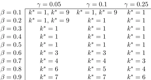
[image:26.595.125.477.127.290.2]γ = 0.05 γ = 0.1 γ = 0.25
β= 0.1 k∗= 1, k∗= 9 k∗= 1, k∗ = 9 k∗ = 1
β= 0.2 k∗= 1, k∗= 9 k∗= 1 k∗ = 1
β= 0.3 k∗= 1 k∗= 1 k∗ = 1
β= 0.4 k∗= 1 k∗= 1 k∗ = 1
β= 0.5 k∗= 1 k∗= 1 k∗ = 1
β= 0.6 k∗= 3 k∗= 3 k∗ = 1
β= 0.7 k∗= 4 k∗= 4 k∗ = 3
β= 0.8 k∗= 6 k∗= 5 k∗ = 4
[image:27.595.123.376.126.260.2]β= 0.9 k∗= 7 k∗= 7 k∗ = 6
Table 5: Equilibrium mall sizes for several values ofβ and γ. The number of firms,n, is fixed to 10.
Onceγ,β and nare fixed, a table with profits for different mall sizes is suf-ficient to find the equilibrium mall size. Take for example the casen= 10, γ = 0.1 andβ= 0.1, which is the left panel in table 4. When no mall exists, profits are 1.2303(ct+ce). When a shop decides to deviate and join another
shop, it will make profits πm
2 = 1.2123(ct+ce). These profits are below
1.2303(ct+ce) and thus k = 1 is an equilibrium. This is indicated in the
table by bold profits. For 2≤k≤8, it is profitable for a mall shop to leave the mall: πm
k < πki−1. Whenk= 9, a mall shop has profits 1.1203(ct+ce).
Leaving the mall would give smaller profits (1.1194(ct+ce)), so a mall shop
has no incentive to deviate. An isolated shop has profits 1.1123(ct+ce)
and joining the mall would give profits of 1.1073(ct+ce). An isolated shop
therefore has no incentive to join the mall and consequentlyk= 9 is another equilibrium (denoted in bold). Fork = 10, a mall shop would find it prof-itable to leave the mall, sok= 10 is not an equilibrium. In the middle and right panel of table 4 the same analysis gives the equilibria that are denoted by bold numbers.
Table 5 gives equilibrium mall sizes for different values ofβandγ, keepingn fixed to 10. To understand the intuition behind the results in this table, first consider the incentives of mall and isolated shops to relocate. A mall shop that leaves the mall loses some of its captive consumers, but at the same time it can set a higher maximum price (rki instead of rmk). On its own, this is not sufficient to leave the mall: in section 4 it has been shown that πkm > πik. But when a shop leaves the mall, the mall size decreases. This lowers 1−xk
n−k and increases the reservation prices. This magnifies the positive
the maximum price it can ask is lower. These two effects on their own would be sufficient to join the mall (πki < πkm), but once again joining the mall changes the size of the mall. This will decrease xk
k and decrease the
reservation prices. Both of these effects negatively affect the profits of a deviating isolated shop, such thatπik> πmk+1 is possible.
Whenβ is high andk is small, xk
k is very high. Intuitively, when the travel
costsctare large, many consumers prefer the mall. If joining the mall would
not affect the mall size, isolated shops would have a large incentive to join the mall and capture this large share of non-shoppers, instead of the tiny share of non-shoppers they capture as isolated shop. As a counteracting effect, joining the mall increases the mall size and therefore decreases xk
k
and the reservation prices. But because xk
k is very large from the outset and
1−xk
n−k is very low, an isolated shop can still gain from joining the mall. This
will only stop when the mall size has grown large and xk
k is relatively small.
Thus, for highβ the equilibrium mall size is fairly large.
When the fraction of shoppers, γ, is large, the only reason for an isolated shop to join the mall is not so important. An isolated shop will join the mall when it leads to a large increase in captive consumers, xk
k. When γ is
large, many consumers are shopping for the best deal and an isolated shop cannot gain many non-shoppers by joining the mall. As a consequence, the equilibrium mall size is smaller whenγ is larger.
For small β there are two possible equilibria: k∗ = 1 and k∗ = 9. As proposition 5.1 shows, whenβ→0, the difference between mall and isolated vanishes, and shops are indifferent about their location.
An equilibrium withk∗ >1 in general gives lower profits for both firm types than a situation where there is no mall at all. To understand the intuition behind this, take a better look at the most right panel of table 4. Starting from a situation with no mall it is profitable to join two shops. These shops will attract much more non-shoppers than when they were isolated. But the remaining isolated shops suffer from this. Because they lose non-shoppers their profits are much lower than in the case no mall existed. Consequently, isolated shops find it profitable to join the mall. This drives down the mall profits to below the level when there were no mall at all, although the re-sulting mall profits are still higher than the isolated profits in the case of k= 2.
Thus far, I have only considered full search equilibria. In the remainder of this section I will also consider partial search equilibria. This equilibrium type is more complicated to analyze because the profits depend onctandce
in a nonlinear way. Therefore, instead of tables, I will provide several plots of expected profits as a function ofct+ce. Simulations show that the plots of
the profits as function ofct+ce when both full and partial search equilibria
0 0.05 0.1 0.15 0.2 0.25 0.3 0.35 0.4 0
0.02 0.04 0.06 0.08 0.1 0.12
c e+ct
profits
π1 π2m
[image:29.595.124.415.127.363.2]π2i
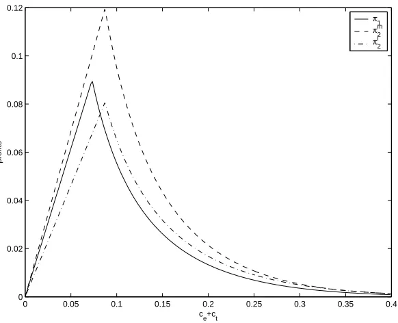
Figure 4: Expected profits as a function of the search costs when all shops are located separately and when there is a mall of two shops. This figure is based on 10 shops, 10 % shoppers and a valuation of the product of 1. The travel costsct are set at 70% of the total search costsct+ce
Section 3. Again, there is a value ofct+ce, called the inflection value, such
that forct+ce below this value the full search equilibrium holds and above
this value the partial search equilibrium holds. The fraction of active non-shoppers,µk, is decreasing in ct+ce and as a consequence the profits in the
partial search equilibrium decrease inct+ce.
Figures 4 and 5 show the expected profits for several values of k. In these figuresγ is set at 0.1, n= 10, β = 0.7 and θ = 1. Figure 4 depicts π1, π2m
and πi2 and figure 5 depicts π2i, π3m and πi3. A first observation is that the inflection point shifts to the right whenkincreases. Note that this also can be inferred from table 2 because the inflection point is simply defined as the value of ct+ce for which rik = θ. Intuitively, competition will be stronger
when more shops are located in the mall. Therefore, more non-shoppers will be tempted to search, shifting the inflection point to the right. The numerical analysis also suggests that fork ≥2 µk ≥µk−1. Intuitively, this
is a consequence of the inflection point shifting to the right. Apart from this, recall that in a partial search equilibrium rik = θ and rkm = θ−ct.
This implies that a change in mall size does not affect the maximum prices the shops can ask. For an isolated shop, joining the mall therefore gives more captive consumers (xk+1
k+1 > 1n instead of
1−xk
n−k <
1
n) and increases the
0 0.05 0.1 0.15 0.2 0.25 0.3 0.35 0.4 0
0.01 0.02 0.03 0.04 0.05 0.06 0.07 0.08 0.09 0.1
ce+ct
profits
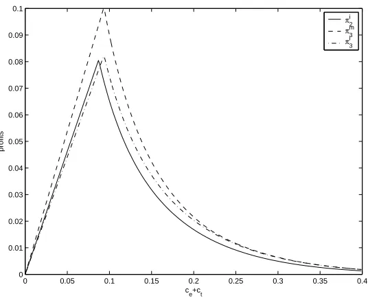
[image:30.595.122.390.126.343.2]π2i π3m π3 i
Figure 5: Expected profits as a function of the search costs when there is a mall of two shops and when there is a mall of three shops. This figure is based on 10 shops, 10 % shoppers and a valuation of the product of 1. The travel costsct are set at 70% of the total search costsct+ce
Therefore, it seems that for large enough values ofct+ceπmk+1≥πki. Figures
4 and 5 indeed show this. To save space, figures of the profits fork >3 are not included in the paper, but they show the same pattern. Thus, for large enough values ofct+ce, n= 10, γ = 0.1, θ= 1 andβ = 0.7 isolated shops
have an incentive to join the mall and the only possible equilibrium is one that has no isolated shops at all (k=n). Simulations for other parameter values give the same result.
7
Conclusion
In this setup, isolated shops will not raise their prices too high. If the differ-ence between the isolated prices and mall prices gets too large, non-shoppers who initially visited an isolated shop will continue to search. Moreover, by setting a low price, an isolated shop can attract the shoppers. As a conse-quence of this, isolated shops attract some share of non-shoppers, which is a necessary condition for an isolated shop to exist in equilibrium.
The location choice of shops is driven by several different factors. First, mall shops attract more non-shoppers per shop than isolated shops. This gives an incentive for isolated shops to join a mall. Second, when an isolated shop joins the mall, the mall size increases and the number of non-shoppers per mall shop decreases. This dampens the first effect. Third, isolated shops can set a slightly higher maximum price than mall shops. This gives a mall shop an incentive to leave the mall. And, fourth, if a mall shop leaves the mall, the competition in the mall decreases and consequently all prices in the market (both mall and isolated prices) increase. These four factors work in different directions. The numerical results in this paper show that there is no dominant effect and mall and isolated shops can coexist.
References
Baye, M.R. and Morgan, J. ”Information gatekeepers on the internet and the competitiveness of homogenous product markets.”American Economic Review, Vol. 91 (2001), pp. 454-474.
Dudey, M. ”Competition by choice: the effect of consumer search on firm location decisions.”American Economic Review, Vol. 80 (1990), pp. 1092-1104.
Dudey, M. ”A note on consumer search, firm location choice, and welfare.”
Journal of Industrial Economics, Vol. 41 (1993), pp. 323-331.
Fischer, J.H. and Harrington, J.E. ”Product variety and firm agglomera-tion.”The RAND Journal of Economics, Vol. 27 (1996), pp. 281-309.
Gehrig, T. ”Competing markets.” European Economic Review, Vol. 42
(1998), pp. 277-310.
Hotelling, H. ”Stability in competition.” The Economic Journal, Vol. 39 (1929), pp. 41-57.
Janssen, M.C.W., Moraga-Gonzalez, J.L. and Wildenbeest, M.R. ”Truly costly sequential search and oligopolistic pricing.”International Journal of Industrial Organization, Vol. 23 (2005), pp. 451-466.
Janssen, M.C.W. and Parakhonyak, A. ”Consumer search with costly re-call.” Discussion Paper no. 2008-002/1, Tinbergen Institute, Erasmus Uni-versity Rotterdam, 2008.
Konishi, H. ”Concentration of competing retail stores.” Journal of Urban Economics, Vol. 58 (2005), pp. 488-512.
Stahl, D.O. ”Oligopolistic pricing with sequential consumer search.” Amer-ican Economic Review, Vol. 79 (1989), pp. 700-712.
Stahl, K. ”Differentiated products, consumer search, and locational oligopoly.”Journal of Industrial Economics, Vol. 31 (1982), pp. 97-113.
Stahl, K. ”Location and spatial pricing theory with nonconvex transporta-tion cost schedules.” The Bell Journal of Economics, Vol. 13 (1982), pp. 575-582.