Munich Personal RePEc Archive
Determinants of the long-run growth
rate in the South-Asian countries
Rao, B. Bhaskara and Cooray, Arusha
November 2010
Online at
https://mpra.ub.uni-muenchen.de/26493/
4-11-10
Determinants of the Long-Run Growth Rate in the South-Asian Countries
B. Bhaskara Rao
School of Economics and Finance
University of Western Sydney, Sydney, Australia
[email protected] Arusha Cooray
School of Economics
University of Wollongong, Wollongong, Australia
Abstract
This study uses the extreme bounds analysis of Leamer (1983) to identify some robust determinants of
the long-run growth rate in seven South-Asian countries. The relationships between the two are
estimated using panel data. We also consider some methodological issues concerning the
specification. It is argued that the frequently used specification of the growth equation by the
cross-country studies is inappropriate for estimating the long-run or steady state growth effects of variables
such as the investment ratio. We use an alternative specification. Since the steady state growth rate in
theoretical growth models depends on total factor productivity (TFP), we estimate the long-run
growth effects of variables by analysing the determinants of TFP. This approach is suggested by a few
influential economists and has been used by Senhadji (2000).
JEL: O11
1. Introduction
Empirical growth equations select a few explanatory variables from a large list of potential
growth affecting variables. However, this selection often is ad hoc and the results are likely
to be sensitive to the selected variables. A solution to this problem is to use first the extreme
bounds analysis (EBA) of Leamer (1983) to identify a few robust determinants of the growth
rate and then estimate the growth equation with these robust variables. Levine and Renelt
(1992) and Sala-I-Martin (1997a and 1997b) have shown how to identify such robust
variables with EBA. We follow their procedures to identify the key determinants of the
long-run growth rate for South-Asia. Our sample consists of data from seven South-Asian
countries for the period 1970 to 2008. These are Bangladesh, Bhutan, India, Maldives, Nepal,
Pakistan and Sri Lanka and are selected for two reasons. Firstly, compared to panel data
studies on the East-Asian countries, South-Asia has received relatively less attention and this
paper partly fills this gap. Secondly, our approach and methodology differ from the existing
procedures in the empirical growth literature. We shall argue that the specification and
methodology in the existing cross-country studies are inappropriate for estimating permanent
growth effects of explanatory variables. Therefore, it is appropriate to determine the
robustness of the selected variables and then estimate the growth equations with the robust
determinants. We illustrate the use of our approach and methodology for estimating the
long-run and permanent growth effects of the determinants. We mean that the long-long-run and
permanent growth effects are the same as the the steady state growth rate (SSGR) of the
theoretical growth models. These terms will be used synonymously in this paper.
The structure of this paper is as follows. Section 2 presents and discusses some key
economic features of the South-Asian countries. Section 3 examines the methodological
issues on the specification and estimation of cross-country growth equations. Section 4
consists of four subsections. Firstly, EBA is used to evaluate the robustness of explanatory
variables. Secondly, estimates of the growth effects of selected determinants are presented in
this section. Thirdly, the policy implications of our estimates are also discussed. Section 5
concludes.
2. Country Characteristics
South-Asia comprises a heterogeneous group of countries faced with a number of obstacles
such as conflict, corruption and high fiscal deficits. An early phase of growth was initiated
from 1950-1970 by planned industrialization based on a strategy of import substitution and
widespread protection, which led to inefficiency and stagnation. A growth revival took place
in 1980s and 1990s following a shift towards an export-led industrialization strategy. A series
of economic reforms were undertaken under the auspices of the IMF and the World Bank in
Sri Lanka in the 1970s, Bangladesh and Pakistan in the 1980s, India, Nepal and Bhutan in the
in 1990s. Liberalisation involved trade and industrial sector reforms and financial sector
deregulation. A number of direct export incentive schemes were introduced and foreign direct
investment was encouraged through the establishment of export processing zones. There has
also been a significant increase in migrant remittances with remittances being a main source
of external financing into these economies following economic reform. In the years following
liberalisation, the growth rates of these countries have accelerated, in particular, that of India.
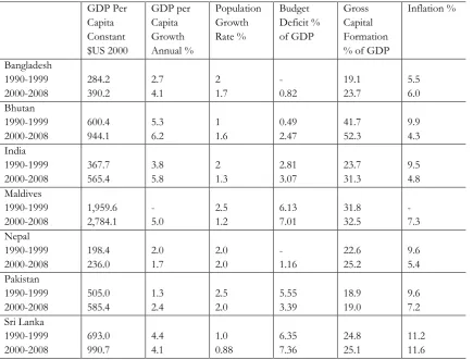
Gross capital formation in these countries as a percentage of GDP has increased, and
population growth has fallen over the 1990-99 to 200-08 period (see Table 1). Although
inflation rates in South-Asia are relatively high, they remain below the developing country
average (Devarajan and Nabi, 2006). There has in addition, been an increase in the female
enrolment ratio leading to a narrowing of the differential between male and female enrolment
ratios in the educational institutions over the 1970-2008 period. Given the progress made by
this region in the recent past, we attempt to identify the variables that are robust in the growth
Table 1: Some Country Characteristics GDP Per Capita Constant $US 2000 GDP per Capita Growth Annual % Population Growth Rate % Budget Deficit % of GDP Gross Capital Formation % of GDP
Inflation % Bangladesh 1990-1999 2000-2008 284.2 390.2 2.7 4.1 2 1.7 - 0.82 19.1 23.7 5.5 6.0 Bhutan 1990-1999 2000-2008 600.4 944.1 5.3 6.2 1 1.6 0.49 2.47 41.7 52.3 9.9 4.3 India 1990-1999 2000-2008 367.7 565.4 3.8 5.8 2 1.3 2.81 3.07 23.7 31.3 9.5 4.8 Maldives 1990-1999 2000-2008 1,959.6 2,784.1 - 5.0 2.5 1.2 6.13 7.01 31.8 32.5 - 7.3 Nepal 1990-1999 2000-2008 198.4 236.0 2.0 1.7 2.0 2.0 - 1.16 22.6 25.2 9.6 5.4 Pakistan 1990-1999 2000-2008 505.0 585.4 1.3 2.4 2.5 2.0 5.55 3.39 18.9 19.0 9.6 7.2 Sri Lanka 1990-1999 2000-2008 693.0 990.7 4.4 4.1 1.0 0.88 6.35 7.36 24.8 25.1 11.2 11.6
3. Specification and Estimation
3.1 Introduction
In cross-country studies, the dependent variable usually is a five or ten-year average growth
rate of per capita income. It is regressed on the initial level of per capita income, some
selected variables with growth effects and control variables. The general form of the
specifications in pure cross-section and panel data studies are as follows.
lnyit (1 ) lnyi0Xit Zitit (1)
lnyit (1 ) lnyit1Xit Zit it (2)
where ln y the average or annual growth rate of per capita income, lnyi0 initial per capita income,lnyt1one panel lagged level of per capita income, X set of explanatory variables of interest, Z control variables, and error term with the classical properties.
Theiandtsubscripts are, respectively, for the cross-section and time series dimensions. For
ease of exposition we assume that X andZvectors consist of only one variable each.
Equation (1) is used in the pure cross-country empirical work, where the time series
dimension is one. The dependent variable in (1) is the average growth rate over the whole
sample period and X and Zare averages over the entire sample period. The well-known
extension to the Solow model by Mankiw, Romer and Weil (1992, MRW) is based on this
methodology and specification. Equation (2) is used in many panel data studies and this
approach is now popular with the availability of software for estimation with panel data
methods. The dependent variable is generally the average growth rate over a five-year period
and the explanatory variables are average values over the five-year period. The lagged
dependent variable lnyit1is the level of per capita income of the previous panel. The
pioneering works of Islam (1995) and Barro (1996) are the earliest to use panel data methods
to estimate growth equations.
3.2 Limitations
Some limitations in the existing empirical growth literature, based on equations (1) and (2),
should be noted. Firstly, a drawback is that aggregation reduces variation in the variables
along the time series dimension and may give implausible results. According to Zorn (2007,
cannot.” For this reason there is support for panel data studies rather than pure cross-section studies. Secondly, a common criticism of cross country studies is their basic assumption that
one size fits all. Thirdly, almost all cross country studies use ad hoc specifications, such as in
(1) and (2), to estimate the growth effects of a few selected variables. Cross country studies
explicitly claim that their objective is to estimate the long-run or the permanent growth
effects of X, given that Z is the control variable. As stated before, it is reasonable to interpret
this long-run or permanent growth rate as the steady state growth rate (SSGR) of theoretical
growth models. If this is the main objective, a five-year or ten-year average growth rate is not
a good proxy for the unobservable SSGR. Conceptually SSGR is similar to the natural rate of
unemployment (NRU) and both are to be derived from the estimates of appropriate dynamic
models by imposing the equilibrium or the steady state conditions. Proxying the SSGR with
the annual or some average growth rate is similar to proxying the NRU with the current
period or some average unemployment rate. Consequently, the growth effects of X will be
overestimated in (1) and (2) because average growth rates will also be affected by transitory
growth rates. These transitory growth rates may persist for some time because it takes
decades for the economy to converge even by 50% towards its steady state level of income.1
Although justification is offered for these specifications, there is confusion as to whether
these are valid for estimating the actual growth rate or the effects of X on the SSGR. Fourthly,
many empirical studies state that their specifications are based on some endogenous growth
model. However, they are based on the extensions to the Solow (1956) exogenous growth
model by MRW (1992), Islam (1995) and Barro (1996). In these three works the steady state
solution for the level of per capita income (y*) for the Solow model is derived first and next the partial adjustment equation is used to explain the actual rate of growth.2
ln ( * )
t t
y y y
(3)
1
The justification for using an average growth rate to proxy the SSGR in the cross country studies is that this measure smooths business cycle fluctuations. If this argument is valid, then there is no need to estimate an expectations augmented Phillips curve to derive NRU because some average rate of unemployment that smooths the business cycle effects would also be a valid estimate of NRU.
For estimates on the speed of convergence, see Barro (1996), Sato (1963) and Rao (2006). However, the speed of convergence also depends on the method of estimation. In general, estimates with GMM seem to imply that convergence is faster than estimates with standard panel data methods.
2
With MRW‟s human capital augmented production function, *
y in the Solow model depends
on the investment ratios of physical capital (sK) and human capital (sH). Therefore, it can be
assumed that * ( , ).
K H
y s s Equation (3) is estimated by MRW using cross-sectional data
for the period 1960-1985 and a sample of 98 countries of both developed and developing
countries. The change made by MRW is to replace the continuous time specification in (3)
with the discrete time specification as follows.
0 0
(lnytlny ) lny (sKt, sHt) (4)
where y0is income per worker in the initial year 1960. Therefore, the dependent variable is the proportionate change of per worker income over 1960-1985; see Table V in MRW
(1992). This equation was used by MRW mainly to estimate the speed of convergence of
incomes in developed and developing countries and not to estimate permanent growth
effects of any variables such as sKandsHbecause these ratios have only permanent level
effects and no permanent growth effects on output. Therefore, it is difficult to accept that
permanent growth effects of variables can be estimated with the specification in (4) or its
variants in several cross country studies including Islam (1995) and Barro (1996).
Furthermore, following Barro, later cross country studies have added a number of additional
variables, such as trade openness, financial development and institutional reform, to the function as potential determinants of the steady state level of income. Justification for these additional variables is generally based on some form of endegenous growth model.
Since the dependent variable is the rate of growth of output, estimates of (4) or similar
equations are interpreted as growth equations and the coefficients of the explanatory variables
as their permanent growth effects. However, it is difficult to accept these arguments because
the main objective of MRW in estimating (4) was to test the convergence hypothesis.3 The
transient growth effects in (4) vanish when the economy reaches its steady state growth path.
Therefore, this equation is not appropriate for estimating the permanent growth effects of X.
There are a few additional problems. Specifications derived from endogenous growth
models are difficult to estimate because it is necessary to estimate a system of non-linear
3
dynamic equations with appropriate econometric techniques; see Greiner et. al., (2005) and
Greiner and Semmler (2002). However, there is also no clear-cut evidence that endogenous
growth models can explain observed facts better than simpler exogenous growth models
based on Solow (1956); see Jones (1995) and Parente (2001). Rogers (2003) also observed
that the older neoclassical growth theory continues to provide inspiration to cross-country
studies. Barro (1996, p. 4) noted, “It is surely an irony that one of the lasting contributions of
endogenous growth theory is that it stimulated empirical work that demonstrated the
explanatory power of the neoclassical growth model.”
Different empirical studies select different explanatory variables from a large number of
potential explanatory variables. Durlauf, Johnson, and Temple (2005) have found that the
number of such potential growth improving variables used in various empirical works is as
many as 145. There is no endogenous growth model in which the specification to estimate the
permanent growth effects uses more than one or two growth enhancing and control variables.
Additional explanatory variables are often included on a heuristic rather than a theoretical
basis if they are supposed to have some potential externalities.
Cross-country studies also used different methods of estimation. Pure cross-section
studies use OLS and panel studies use the standard fixed and random effects panel methods.
More recently, generalised method of moments (GMM) and the system GMM (SGMM)
methods are also used. GMM and SGMM are used to eliminate country specific fixed effects
and to minimise biases due to endogeneity by instrumenting the explanatory variables. There
are hardly any cross-country studies that use time series based panel methods. We postpone
any evaluation of the relative merits of these alternative estimation methods due to space
constraints.
3.3 Alternative approaches
In light of the above criticisms, two alternative approaches are worth consideration.
Following Barro, many empirical works have treated equation (4) as if it were a growth
equation to estimate the permanent growth effects of variables. Since we have argued that (4)
is not suitable for this purpose, the question of what factors determine permanent growth
effects and how these growth effects should be estimated remains unexplained. There are a
few alternative methods to analyse the determinants of the permanent growth rate and they
depend on the selected theoretical growth model. The simpler methods are based on
growth models and the interest reader may refer to Greiner et. al., (2004). In this paper we
shall consider two approaches based on the Solow model.
In Solow (1956) the SSGR equals the rate of growth of technical progress (TFP). A
well-known weakness of this model is that it does not explain what factors determine TFP and the
endogenous growth models of the 1980s are developed to fill this gap. Two types of factors
that determine TFP can be distinguished viz., growth factors that need no additional resources
and those that need additional resources. The first is the manna from heaven type, of which
the classic example is Arrow‟s (1962) learning by doing (LBD). A typical example of the second type is expenditure on research and development (R&D). While the Solow model can
easily be extended to include the manna from heaven type determinants of TFP, a two-sector
endogenous growth framework is appropriate for estimating the permanent growth effects of
variables like R&D. However, empirical works, including Barro (1996), based on equation
(4), have arbitrarily added both categories of variables as determinants of the growth rate.
Edwards (1998), Bernanke and Gurkaynak (2001) and Dollar and Kraay (2004) have
suggested that the permanent growth effects of variables should be estimated by estimating
their effects on TFP. Senhadji (2000) has followed this approach and selected the MRW
human capital augmented Solow (1956) model. He has estimated TFP by conducting a
growth accounting exercise based on Solow (1957) for 88 countries for the period 1960 to
1994. The estimated TFPs are used to compute relative TFPs with respect to the USA and
this ratio is regressed on some potential explanatory variables. Subsequently Rao and Hassan
(2010a and 2010b) have also followed this approach to estimate the determinants of the
long-run growth rate in Bangladesh. They have used the growth accounting approach of Senhadji
in Rao and Hassan (2010a). In Rao and Hassan (2010b) a simpler one-step method is used,
which is explained below.
3.4.TFP Determinants: An Alternative Method
We shall use the standard model of Solow. For simplicity, we shall ignore human capital and
the cross-section dimension. With this simplification, the Cobb-Douglas production function
with constant returns and Harrod neutral technical progress is as follows.
where A is the stock of knowledge, Y is income , K is capital and L is employment. The
solution for the steady state level of per worker income is:
1 * s
y A
d g n
(6)
where y( / ).Y L The steady state growth rate (SSGR), when the parameters in brackets
remain constant, is:
lny* lnAg (7)
In the Solow model although the stock of knowledge (A) is assumed to be exogenous, in the
empirical work it is commonly assumed that A grows at a constant rate of g, i.e.,
At A e0 gt (8)
where A0is the stock of knowledge in the initial period. It is reasonable to extend the model
by making the stock of knowledge depend, besides time, on other variables,Zi,which are
found to be growth affecting by some endogenous models.4 To extend the Solow model we
assume that g in (8) is a function of the Z variables, so that:
( 0 )
0 1...
j jt
g g Z t t
A A e j m (9)
The advantage of this extension is that it is relatively easy to estimate the permanent growth
effects of Zjwith the panel or country specific time series data. In (9) TFP is:
0 gj j
gg
Z where g0captures the effects of the neglected but trended variables. Thus, the long-run growth rate depends on the levels of the Zj variables, as in the endogenousgrowth models. The coefficients g jj( 0... )m should be significant if the Zj variables have
externalities.
4
While in country specific studies it is not possible to include more than a handful of
variables in Zj due to limited sample sizes, in cross country studies it is possible to do this
because of more observations. In their EBA Levine and Renelt (1992) find that the only
robust explanatory variable in growth regressions is the investment ratio. In contrast, using a
less stringent version of EBA, Sala-I-Martin (1997a ad 1997b) found that out of about 62
explanatory variables that have been used by various empirical studies, 25 variables have
robust effects on growth of which three are MUST variables.5 However, both studies have
some limitations because they have used the standard specification of the growth equation
based on (4) and pure cross-section OLS method of estimation. The limitations of the
specification of the growth equation are noted by Sala-I-Martin. He has noted that “The
problem faced by empirical growth economists is that growth theories are not explicit enough
about what variables belong in the „true‟ regression.”
In light of the above discussion and for pragmatic reasons, it seems necessary to follow
a few methodological guidelines in growth empirics. If several works based on alternative
methodologies, data sets, estimation methods and different explanatory variables indicate, for
example, that while the investment rate and trade openness have positive and significant
growth effects and the ratio of government expenditure and inflation have negative growth
effects, our confidence in their growth effects will increase. In further research on the growth
effects of a new variable, for example, health or schooling, these four variables should be
included as the MUST variables. Many empirical studies follow more or less such a
methodology in estimating not only growth equations but also other relationships. However,
the findings by known experts and published papers in prestigious professional journals
generally receive more weight in the justification for the choice of specifications and
explanatory variables. We shall follow this practice for the choice of explanatory variables. If
the main objective is to estimate the permanent growth effects of these explanatory variables,
alternative specifications and procedures, which are discussed in the previous sections, are
more appropriate than the present specifications based on equation (4).
5
4. Empirical Results
4.1 Introduction
In this section, we first use our alternative specification and approach for estimating the
permanent growth effects of thirteen variables. These are similar to those used by Levine and
Renelt (1992) and Senhadji (2000). Instead of selecting some to estimate their growth effects,
we apply EBA to check how many are robust in their effects with the methods used by Levine
and Renelt (1992) and Sala-I-Martin (1997a and 1997b). A comparison between our findings
with the results in these previous works would be useful to see their differences. Since in the
EBA several combinations of three explanatory variables are used to evaluate their
robustness, it is necessary to estimate our specification (5) with all the variables that are
expected to be robust. The specification of our extended production function based on (5) and
(9), with cross-section and time series subscripts, is as follows. However, it is convenient to
assume Hicks neutral technical progress instead of Harrod neutral technical progress and it
makes no difference for the results. Equation (5) with these changes is as follows.
,0
( )
,0 +
i jit jitt it
g g Z T
it i it
y A e k (10)
,0 0 1 1 13 13
ln
ln it ln i ( i it it it it)
it it k
y A g g Z g Z T
(11)
Where y( / ),Y L k(K L/ ), Z1it Z13itare variables with growth effects, T time,
0
A initial stock of production knowledge, which may depend on not only education but also
other factors such as resource endowments etc., (see MRW, 1992), icross-section subscript
which is seven in this paper and ttime series subscript which is 39. We assume that the
error term is N(0,2), but its structure differs in the fixed effects estimates.
4.2 Extreme Bounds Analysis
Leamer‟s (1983) EBA is adequately explained by Levine and Renelt and Sala-I-Martin. Therefore, we shall be brief here. Essentially, in EBA all possible combinations of three
explanatory variables are selected and estimates are made with the random effects method. In
these estimates, one or two variables, usually included in many regressions, are retained as
MUST variables in all estimates. In this paper we treat time and capital per worker (k) as the
not change sign in the estimates with all combinations of the three explanatory variables.
With this criterion, they find that only the investment rate is a robust explanatory variable in
growth equations. However, Sala-I-Martin is critical of this criterion because it is too
stringent and a variable becomes fragile even if it changes sign only once. Therefore, he uses
the cumulative distribution functions (CDF) of the estimated coefficients to determine the
robustness of the variable. He selects the 95% probability level as the critical value.
Therefore, a variable becomes fragile only if its coefficient changes sign in more than 5% of
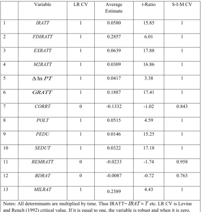
estimates. Table 3 gives EBA results for our 13 variables, with their average estimated values
and the Levine and Renelt and Sala-I-Martin critical values. These estimates are based on 286
combinations of three variables at a time of the 13 selected variables. Altogether 3,718
equations are estimated.
According to Levine and Renelt, a variable is robust if the critical value is 1 and
fragile if it is zero. In Sala-I-Martin, a variable is robust if the critical value is equal to or
more than 95% and fragile otherwise. The thirteen variables selected are, with the expected
signs for their coefficients are: the ratio of investment to GDP (IRAT, +), ratio of foreign
direct investment to GDP (FDIRAT, +), ratio of exports to GDP (EXRAT, +), ratio of M2 to
GDP (M2RAT,+), inflation rate (lnP,), ratio of government consumption expenditure
to GDP (GRAT,), a measure of corruption (CORR, -), a measure of institutional
development (POL, +), primary enrolment ratio (PEDU, +), secondary enrolment ratio
(SEDU, +), ratio of workers‟ remittances to GDP (REMRAT , + ), ratio of budget deficit to
GDP (BDRAT, -) and ratio of military expenditure to GDP (MILRAT, + or -). Some average
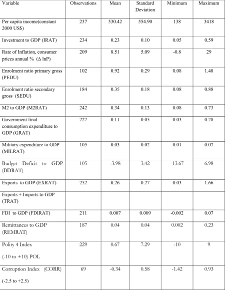
values of the variables are given in Table 2.
Although in the Solow model variables such as IRAT and FDIRAT etc., have only
permanent level effects, these variables may have permanent growth effects if they have
some externalities. Levine and Renelt and Sala-I-Martin‟s EBA showed that IRAT is a robust
variable in growth equations, in spite of our reservations on the specification of the growth
equation. Therefore, it is of interest to see if IRAT has robust growth effects with our
alternative specification. EXRAT is used as a proxy for trade openness. When we used the
ratio of exports plus imports to GDP (TRAT ), which is a frequently used proxy for trade
openness, its coefficient was negative and fragile. This may be due to the dominance of the
negative growth effects of imports. M2RAT is a proxy for financial development and many
proxies for government‟s economic policies. CORR and POL measure institutional quality.
Remittance by migrant workers (REMRAT ), which are a rising proportion of GDP in the
South-Asian countries, may have a small indirect effect on the growth rate; see Rao and
Hassan (2010 a,b). Education at the primary and secondary levels (PEDU and SEDU) capture
the growth effects of human capital. It is hard to say whether MILRAT has a positive or
negative growth effect. It will have a negative growth effect if resources are diverted from
productive sectors to the defence sector. However, its contribution to growth will be positive
if it increases infrastructure investment, adoption of new technologies and improves political
Table 2: Descriptive Statistics
Variable Observations Mean Standard
Deviation
Minimum Maximum
Per capita income(constant 2000 US$)
237 530.42 554.90 138 3418
Investment to GDP (IRAT) 234 0.23 0.10 0.05 0.59
Rate of Inflation, consumer prices annual % (lnP)
209 8.51 5.09 -0.8 29
Enrolment ratio primary gross (PEDU)
102 0.92 0.29 0.08 1.48
Enrolment ratio secondary gross (SEDU)
184 0.35 0.18 0.08 0.88
M2 to GDP (M2RAT) 242 0.34 0.13 0.08 0.73
Government final
consumption expenditure to GDP (GRAT)
227 0.11 0.05 0.03 0.28
Military expenditure to GDP (MILRAT)
105 0.03 0.02 0.01 0.07
Budget Deficit to GDP (BDRAT)
105 -3.98 3.42 -13.67 6.98
Exports to GDP (EXRAT) 252 0.26 0.27 0.03 1.66
Exports + Imports to GDP (TRAT)
FDI to GDP (FDIRAT) 211 0.007 0.009 -0.002 0.07
Remittances to GDP (REMRAT)
187 0.04 0.04 0.002 0.23
Polity 4 Index
(-10 to +10) POL
229 0.67 7.29 -10 9
Corruption Index (CORR)
(-2.5 to +2.5)
69 -0.34 0.58 -1.42 0.93
The EBA results in Table 3 show that both criteria give similar results. According to
fragile, while according to Sala-I-Martin‟s criterion REMRAT is robust just at the margin but
CORR and BDRAT are fragile. Our results based on these two criteria are much closer than
the wide gap in the results Levine and Renelt and Sala-I-Martin with the conventional
specification. The signs of the coefficients on inflation, government expenditure and
remittances are contrary to prior expectation and it is hard to accept that the coefficient of
military expenditure could be positive. These unexpected results are not uncommon. In
Sala-I-Martin (1997) the coefficients of some variables such as civil liberties, public investment
[image:17.595.96.500.276.701.2]share, political assassinations and trade openness etc., have the wrong signs.
Table 3: Extreme Bounds Analysis
Variable LR CV Average
Estimate
t-Ratio S-I-M CV
1 IRATT 1 0.0580 15.85 1
2 FDIRATT 1 0.2857 6.01 1
3 EXRATT 1 0.0639 17.88 1
4 M2RATT 1 0.0309 16.86 1
5 lnPT 1 0.0417 3.38 1
6 GRATT 1 0.1887 17.41 1
7 CORRT 0 -0.1332 -1.02 0.843
8 POLT 1 0.0515 4.59 1
9 PEDU 1 0.0146 15.25 1
10 SEDUT 1 0.0322 17.18 1
11 REMRATT 0 -0.0233 -1.74 0.958
12 BDRAT 0 -0.0087 -0.72 0.763
13 MILRAT 1 0.2389 4.43 1
Notes: All determinants are multiplied by time. Thus IRATT=IRAT T etc. LR CV is Levine
and Renelt (1992) critical value. If it is equal to one, the variable is robust and when it is zero,
the variable is fragile. S-I-M CV is Sala-I-Martin‟s (1997) critical value. When it is 0.95the
4.3 Empirical Results on the Determinants
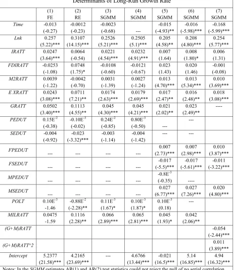
Empirical estimates of equation (11) are reported in Table 4 with the 13 determinants with alternative
panel methods of fixed effects (FE), random effects (RE) and system GMM (SGMM) yielded poor
results. The log of per worker capital (lnk), EXRAT, GRAT and the intercept are significant at the 5% level. RE estimates, with the Swamy and Arora (1972) option, which has better finite sample
properties, give slightly improved results. With this estimate ln ,k FDIRAT, EXRAT, GRAT , POL,
SEDU and MILRAT are statistically significant. However, POL, SEDU and MILRAT have the wrong
sign. It is surprising that IRAT, which found to be the only robust determinant of growth by Levine
and Renelt, is not significant in all these three estimates. The Breusch and Pagan test with the null for
the RE model over FE model is insignificant. The computed test statistics is 2(1) 1.14 with a p-value of 0.286. Therefore, RE estimates seem to be preferable to FE estimates. These preliminary
results are not reported to conserve space.
Next, we estimated (11) without the three fragile variables CORR, REMRAT and BDRAT but
the results are similar. The coefficient of inflation remained still positive and that of investment ratio
is insignificant. We deleted these two variables and the FE and RE estimate with the Swamy and
Arora option are reported in columns (1) and (2) of Table 4. The Breusch-Pagan test statistic
(2(1) 1.16 with p-value of 0.282) cannot reject the null of RE. To minimise the endogenous variable bias and the likely persistence in the variables, we reestimate this equation with SGMM after
limiting the number of instrumental variables; see Roodman (2009) for this requirement. Two SGMM
estimates without intercept (but with trend) and with intercept (but without trend) are made to see if
trend is significant. These two SGMM estimates are reported in columns (3) and (4) of Table 4.
It can be seen from the results in Table 4 that the coefficient of trend is insignificant in the three
equations with trend. The coefficient of capital, share of profits, is low at 0.17 in the FE estimate but
near its stylised value of one third in the RE estimate in column (2). However, in the two SGMM
estimates it is around 0.25 and this is a plausible value for the developing countries. The higher
estimate in column (2) may be due to the endogeniety of capital stock. For a similar reason the
Table 4: Empirical results
Determinants of Long-Run Growth Rate
(1) FE (2) RE (3) SGMM (4) SGMM (5) SGMM (6) SGMM (7) SGMM
Time -0.013 (-0.27)
-0.0012 (-0.23)
-0.0023
(-0.68) ---
-0.015 (-4.93)** -0.016 (-5.98)*** -0.168 (-5.99)***
Lnk 0.257
(5.22)*** 0.3107 (14.15)*** 0.2526 (5.21)*** 0.2505 (5.1)*** 0.205 (4.58)** 0.208 (4.80)*** 0.254 (5.77)***
IRATT 0.0247 (3.64)*** 0.0064 (-0.54) 0.0221 (4.54)*** 0.0232 (4.91)*** 0.007 (1.64) 0.008 (1.80)* 0.006 (1.31)
FDIRATT -0.0253 (-1.08) 0.0748 (1.75)* -0.0108 (-0.60) -0.0121 (-0.67) 0.023 (1.43) 0.020 (1.46) -0.001 (-0.08)
M2RATT 0.0039 (-1.22) -0.0042 (-0.70) 0.0031 (-1.39) 0.0027 (-1.24) 0.013 (4.70)*** 0.013 (5.34)*** 0.010 (3.69)***
E XRATT 0.0243 (3.08)*** 0.0711 (7.21)** 0.0174 (2.63)*** 0.0179 (2.69)*** 0.017 (2.47)** 0.016 (2.48)** 0.018 (3.08)***
GRATT 0.0502 (3.40)*** 0.1113 (4.55)** 0.045 (4.30)*** 0.045 (4.21)*** 0.021 (2.02)** 0.023 (2.49)** ----
PEDUT 0.15E-2 (-0.38) -0.10E-3 (-0.02) 0.24E-2 (-0.85) 0.80E-3 (-0.50) --- ---
SEDUT -0.004 (-0.92) -0.023 (-3.32)*** -0.003 (-1.14) -0.004 (-1.42) --- --- FPEDUT --- --- --- --- 0.007 (2.73)*** 0.007 (2.98)*** 0.010 (3.87)*** FSEDUT --- --- --- --- -0.017 (-5.5)*** -0.017 (-5.61)*** -0.011 (-3.22)*** MPEDUT --- --- --- --- -0.8E-3
(-0.35) ----
MSEDUT --- --- --- --- 0.027 (6.77)*** 0.027 (7.26)*** 0.020 (4.80)***
POLT 0.10E-3 -1.46 -0.88E-2 (-2.28)** 0.11E-3 (1.67)* 0.10E-3 (1.87)* 0.10E-3 (0.18) ---
MILRATT 0.0475 0.1116 0.066 0.065 0.045 0.042
-1.59 (2.28)** (2.89)*** (2.81)*** (1.93)* (2.06)**
(G+M)RATT -0.054
(-2.44)***
(G+M)RATT^2 0.011
(3.89)***
Intercept 5.2377 (21.58)***
4.2165 (23.69)***
--- 4.6766
(13.44)*** -0.021 (16.5)*** 5.14 (16.85)*** 4.94 (16.32)***
At this stage it can be said that SGMM estimates are preferable to RE estimates because this
estimate minimises biases due to endogeniety and persistence in the variables. Of the two SGMM
estimates, the one in column (4), without trend, is preferable because its pseudo
__ 2
,
R at 0.881
is marginally higher than the estimate in column (3) of 0.804.6 In subsequent estimates we
shall use variants of this specification and estimation.
Estimates of the preferred equation in column (4) are not entirely satisfactory. The
coefficients of FDIRAT and SEDU are negative and insignificant. The coefficient of PEDU,
although has a positive sign, is insignificant. The positive and significant coefficient for
MILRAT is difficult to justify. Since the coefficients of trend, primary and secondary
enrolment ratios are insignificant, we have tested in a different way for the significance of
trend by replacing the two enrolment ratios with the components of the enrolment ratios viz.,
female and male enrolment ratios in primary schooling (FPEDUT and MPEDUT) and female
and male enrolment ratios in secondary schooling (FSEDUT and MSEDUT). These estimates
are reported in column (5). Of the four enrolment ratios only the male enrolment ratio in
primary schooling is insignificant in column (5). The coefficient of female enrolment ratio
in secondary schools is negative and the coefficient of political institutions became
insignificant. In column (6) estimates of this equation, without the two insignificant variables
MPEDU and POL, are reported. It can be seen that there are no significant changes in the
estimates of the parameters in the last two columns.
We shall use the estimates in column (6) for a few conclusions. All the coefficients,
except FDIRAT, are significant at the five or ten percent levels. The coefficient of FDIRAT
has the expected positive sign and significant at about 14.5 percent level. This and the
equation in column (5) imply that TFP is negative at about 1.5 percent per year. This high
negative value may be due to stringent bureaucratic systems and closed economy policies in
South-Asian countries.7 India opened up its economy and implemented market reforms only
in the 1990s. In general, the permanent growth effects of many variables are found to be
much less than in the previous studies with conventional specifications of the growth
equation. For example, the coefficient of IRAT, which is highly significant in Levine and
6
These are generated by obtaining the predicted values of the dependent variable of the two SGMM estimates.
7
In two country specific studies, Rao and Vadlamannati (2010) for India and Rao and Hassan (2010) for
Renelt and Sala-I-Martin with coefficients of about 0.17 (slow growers) to 0.14 respectively,
has a much lower coefficient of 0.008 in our estimate. Our estimate implies that the
permanent growth effect of the investment ratio is about 0.01 percentage points at most and
not as high as in Levine and Renelt. As pointed out before, the conventional specification of
the growth equation overestimates the permanent growth effects because it also captures the
transitory growth effects. Male secondary school enrolments (MSEDU) has a much larger
growth effect of about 0.03. The growth effects of progress of financial sector (FDIRAT) and
exports (EXRAT) are also higher than IRAT. Only female primary school enrolments
(FPEDU) has a similar growth effect to IRAT.
Some less plausible estimates are the relatively large and positive growth effects of
government expenditure (GRAT ) and military expenditure (MILRAT).8 When GRAT is
replaced with the ratio of budget deficit (BDRAT), its coefficient is insignificant but remains
positive. Allowing for nonlinear effects and interaction terms with inflation does not make
the coefficients of GRAT and MILRAT negative or insignificant. Both these ratios are
somewhat correlated with a correlation coefficient of 0.71. Therefore, we added these two
ratios and allow for a combined nonlinear effect with the square of this combined term.
Estimates with these changes are in column (7) of Table 4. It can be seen that the coefficient
of the combined term is negative and significant. The nonlinear effect of this combined term
implies that its effects are negative until it reaches an implausible value of 260 percent
whereas the sample average is only 12.5 percent. However, the coefficient on IRAT becomes
insignificant and the profit share increases slightly. There are no other significant changes in
the estimates of other coefficients. Therefore, the effects of GRAT and MILRAT need further
analysis but this is beyond the scope of the present paper.
4.4 Policy Implications
8
One of the important objectives of analysing the determinants of long-run permanent growth
is to understand the policy options which may increase the long-run growth rate. The average
per worker income growth rate of the South-Asian countries is around 2.33 percent, which is
about the same as the growth rate of per capita income. If this permanent growth rate needs to
be increased by one percent, i.e., to make the current rate of 2.33 into 3.33 percent, what are
the policy options? Although this target can be achieved with some alternative combinations
of policy options, our subjective preference is as follows. This target can be achieved by
emphasising the male and female school enrolment ratios. It is possible by increasing by 20%
the current ratios of IRAT, EXRAT, M2RAT, and by increasing FPEDU and MSEDU by 55%.
If all these ratios are increased by 20%, the permanent growth rate will increase only by half
percent. In our view both policy options are not difficult to implement.
5. Conclusions
Using the EBA we have identified some robust determinants of the long-run growth rate in
seven South-Asian countries. We found that these robust determinants, with the exception of
FDI, are all statistically significant at the 5% or 10% level. The evidence suggests that the
growth effects of investment are relatively smaller compared to other determinants like
education. This may be due to investments taking place in the traditional and less innovative
sectors. More growth enhancing determinants are female primary enrolment and male
secondary enrolment ratios. Similarly, our results suggest that countries with a larger and
more active financial sector grow faster. Government expenditure has a positive effect on
economic growth. This is possibly due to the fact that the government is the main provider of
education, health and other services in the South-Asian countries. Similarly military
expenditure has a positive impact on growth possibly due to investment taking place in
infrastructure and capital goods.
We have also argued that it is important to distinguish between the transient growth
effects from the permanent and long-run growth effects of the determinants of growth.
Currently used specifications in the cross-country studies are likely to overestimate the
growth effects of the determinants by failing to make this distinction. We hope that our
specification and methodology would encourage other investigators to avoid overestimating
Data Appendix
Variable Source
Per capita income(constant 2000 US$) World Development Indicators 2010
Investment to GDP (IRAT) World Development Indicators 2010
Rate of Inflation, consumer prices annual % (lnP)
World Development Indicators 2010
Enrolment ratio primary (PEDU) World Development Indicators 2010
Enrolment ratio secondary (SEDU) World Development Indicators 2010
M2 to GDP (M2RAT) World Development Indicators 2010
Government final consumption expenditure to GDP (GRAT)
World Development Indicators 2010
Military expenditure to GDP (MILRAT) World Development Indicators 2010
Budget Deficit to GDP (BDRAT) World Development Indicators 2010
Exports to GDP (EXRAT) World Development Indicators 2010
FDI to GDP (FDIRAT) World Development Indicators 2010
Remittances to GDP (REMRAT) World Development Indicators 2010
Polity 4 Index -10 to +10 (POL) Marshall and Jaggers (2010):
http://www.systemicpeace.org/polity/polity06.ht m#nam
Corruption Index -2.5 to +2.5 (CORR) Kaufmann, Kraay and Mastruzzi (2009): Governance Matters VIII: Governance Indicators for 1996-2008. World Bank Policy Research Working Paper 4978.
Note: World Development Indicators (WDI).
http://databank.worldbank.org/ddp/home.do?Step=2&id=4&DisplayAggregation=N&SdmxSuppor
References
Arrow, K. (1962) The Economic Implications of Learning by Doing, Review of Economic
Studies, 29, 155-173.
Barro, R. J. (1996) Determinants of Economic Growth: A Cross-Country Empirical Study,
NBER WP 5698, National Bureau of Economic Research, Cambridge, MA.
Bernanke, B. S. and Gürkaynak, R. S. (2002) Is Growth Exogeneous? Taking Mankiw,
Romer and Weil Seriously, NBER Macroeconomics Annual, 16, 11-72.
Cass, D. (1965) Optimum Growth in a Model of Capital Accumulation, Review of Economic
Studies, 32, 223-240.
Devarajan, S. and Nabi, I. (2006) Economic Growth in South-Asia: Promising,
Unequalizing…Sustainable? mimeo, World Bank, Washington. Available from
http://siteresources.worldbank.org/SOUTHASIAEXT/Resources/South_Asia_growth_June_2
006.pdf.
Dollar, D. and Kraay, A. (2004) Trade, Growth and Poverty, Economic Journal, 114, F22–
F49.
Durlauf, S. N., Johnson, P. A. and Temple, J. R.W. (2005) Growth Econometrics, in Aghion,
P. and Durlauf, S. (ed.), Handbook of Economic Growth, chapter 8, 555-677, Amsterdam:
North-Holand.
Edwards, S. (1998) Openness, Productivity and Growth: What Do We Really Know?
Economic Journal, 108 (447), 383-98.
Greiner, A., Semler, W. and Gong, G. (2005) The Forces of Economic Growth: A Time Series
Perspective, Princeton, NJ: Princeton University Press.
Greiner, A. and Semmler, W. (2002) Externalities of Investment, Education and Economic
Growth, Economic Modelling, 19, 709-724.
Islam, N. (1995) Growth Empirics: A Panel Data Approach, Quarterly Journal of Economics,
Jones, C. (1995) R&D-Based Models of Economic Growth, Journal of Political Economy,
103 (4), 759-784.
Kaufmann, D, Kraay, A., and Mastruzzi, M. (2009) Governance Matters VIII: Governance
Indicators for 1996-2008. World Bank Policy Research Working Paper 4978.
Koopmans, T. (1965) On the Concept of Optimal Economic Growth, The Econometric
Approach to Development Planning, Amsterdam: North-Holland.
Leamer, E. E. (1983) Let‟s Take the Con Out of Econometrics. American Economic Review 73, 31–43.
Leamer, E. E. (1985) Sensitivity Analyses Would Help. American Economic Review 75,
308–13.
Levine, R. and D. Renelt. (1992) A Sensitivity Analysis of Cross Country Growth
Regressions, American Economic Review, 82, 942-963.
Mankiw, N.G., D. Romer and D. Weil. (1992), A Contribution to the Empirics of Economic
Growth, Quarterly Journal of Economics, 107, 407-437.
Marshall, M. and Jaggers, K. (2010) http://www.systemicpeace.org/polity/polity06.htm#nam.
Parente, S. (2001) The Failure of Endogenous Growth, Knowledge, Technology and Policy,
13, 49-58.
Rao, B.B. (2010) Estimates of the steady state growth rates for selected Asian countries with
an extended Solow model, Economic Modelling, 27, 46-53.
Rao, B. B. (2006) Investment ratio and growth. ICFAI Journal of Applied Economics, 3,
68-72.
Rao, B. B., Gounder, R. and Loeing, J. (2010) The level and growth effects in the empirics of
economic growth: some results with data from Guatemala, Applied Economics, 42,
Rao B. B. and Hassan, G. E. (2010a) Determinants of the Long Run Growth Rate of
Bangladesh, forthcoming, Applied Economics Letters.
Rao B. B. and Hassan, G. E. (2010b) An Analysis of the Determinants of the Long Run
Growth rate of Bangladesh, forthcoming, Applied Economics.
Rao, B. B., Tamazian, A. and Singh, R. (2010) Financial Developments and the Rate of
Growth of Output: An Alternative Approach, forthcoming, Applied Economics.
Rao B. B. and Vadlamannati, K. C. (2010) The Level and Growth Effects of Human Capital in
India, forthcoming, Applied Economics Letters.
Rogers, M. (2003) A Survey of Economic Growth, Economic Record, 79, 112-135.
Romer, P. M. (1986)Increasing Returns and Long-Run Growth, Journal of Political
Economy, 94, 1002-37.
Roodman, D. (2009) A Note on Too Many Instruments, Oxford Bulletin of Economics and
Statistics, 71, 135-158.
Sato, R. (1963) Fiscal Policy in a Neo-Classical Growth Model: An Analysis of Time
Required for Equilibrium Adjustment, Review of Economic Studies, 30, 16-23.
Sala-I-Martin, X. (1997a) I Just Ran Four Million Regressions, NBER Working Paper No.
6252.
Sala-I-Martin, X. (1997b) I Just Ran Four Million Regressions, American Economic Review,
87, 178-183.
Senhadji, A. (2000) Sources of Economic Growth: An Extensive Growth Accounting
Exercise, IMF Staff Papers, 47, 129-157.
Solow, R. M. (1956) A Contribution to the Theory of Economic Growth, Quarterly Journal
ofEconomics, 70, 65-94.
Swamy, P. A. and Arora, S. S. (1972) The exact finite sample properties of the estimators of
coefficients in the error component regression models. Econometrica, 40, 261-275.
Swan, T. (1956), Economic Growth and Capital Accumulation, Economic Record, 32,
Young, A. (1994) Lessons from the East Asian NICs: A Contrarian View, European
Economic Review, 38, 964-973.
Zorn, C. (2007) Notes for “Advanced MLE” Summer 2007. Available only from Professor