Munich Personal RePEc Archive
Capabilities measurement: an empirical
investigation
HASAN, HAMID
La Trobe University
23 June 2009
Online at
https://mpra.ub.uni-muenchen.de/16742/
Capabilities Measurement: An Empirical Investigation
Hamid Hasan*Abstract
Sen’s seminal contribution highlights the importance of positive freedom in the measurement of human welfare. The present paper attempts to measure this freedom aspect in an integrated approach. The main contribution of the paper is the simultaneous estimation of capability, functioning, and conversion efficiency with explicit modeling of
freedom by latent variable modeling approach. The knowledge dimension of
capabilities is modeled and estimated by integrating exploratory and confirmatory statistical methods in a two-stage procedure. In the first stage, Partial Least Squares method is employed to construct latent variable scores. These scores are transformed to relative scores for the sake of comparison and then used to estimate the proposed simultaneous-equation capability model by 3SLS in the second stage. The results show that capability is inversely related to resources and positively related to freedom and functioning. The computed relative capability and freedom inequality ratios are very high whereas relative functioning and efficiency inequality ratios are at a moderate level. The conventional income inequality ratio is lower as compared to the capability dimensions’ ratios and close to the Gini-coefficient. The paper extended the measurement of conversion inefficiency into voluntary and involuntary inefficiency. The paper also suggests criteria for evaluating empirical research within the capability approach
framework.
The paper recommends development of specific survey instruments in order to create better indicators for capability dimensions and use of latent variable modeling for constructing latent variable scores, and their subsequent use in estimation. These findings suggest a capabilities-oriented public and education policies for the enhancement of knowledge dimension of capabilities in particular and human welfare in general. The focus of education policy should be extended from investment-oriented (human capital approach) to value-oriented (human capability approach).
Key words
Capabilities; Freedom; Functioning; Conversion Efficiency; Latent variables; Structural equations model; PLS; LISREL; 3SLS.
JEL Classification D39; D63; I31; I132;
*
1. Introduction
Atkinson (1999, p.186) states: ‘A concept is effective if it causes people to think in a different way’. He refers it to Sen’s concept of capability which opens the door for deontological considerations for the assessment of individual well-being.1 It extends and encompasses the utilitarian (welfarist) and resourcist approaches of well-being evaluation2.
This paper will develop freedoms’ aspect of Sen’s capability approach (CA) theoretically and empirically within the CA framework of thought3. According to Sen (2004, p.21), the idea of freedom is relevant to normative social choice theory, in general, and to the theory of justice, in particular, and provides normative foundations of human rights. Arrow (1999), Atkinson (1999), and Pressman and Summerfield (2000)4 have separately discussed Sen’s major contributions in the fields of social choice, welfare economics and its critique, measurement of economic inequality and poverty, development economics and the implementation of capabilities. This paper is related to the last of these four major contributions.
I will argue in this paper that individual freedom in Sen’s perspective is an extremely significant factor in the evaluation of human welfare that its explicit theoretical and empirical modeling is not only necessary but also urgent since most of the human sufferings in the last decade have been related to this very concept; people are deprived off the kind of life they want to lead. Alkire (2005) emphasizes the need for measuring freedoms. She argues (p.10):
With respect to the measurement of freedom as indicated above, I observe
that the literature to date has focused upon the measurement of functionings, and left
process freedoms – and indeed opportunity freedoms – largely unaddressed thus far.
Freedom in terms of range of choices and autonomy are the basic requirements for justice and measuring the standard of living. It has instrumental as well as intrinsic value and the evaluation on the basis of freedom provides an encompassing measure of well-being.
‘According to Sen’s capability approach, economic and social arrangements should be evaluated
in terms of the freedoms enjoyed by those who live in them’ (Akire, 2005). Sen (1990)
discusses freedom as a focal personal feature for ethical judgment on the lives of persons and compares it to primary goods and liberties (Rawls), rights (Nozick), resources
(Dworkin) among others. In this context, he distinguishes between means and what people can obtain from the means. He argues (p.115):
1
The fundamental theorems of welfare economics do not consider ethical or normative aspects unless modified in a certain way.
2 According to Austrian school of thought, Sen’s framework provides an alternative to neoclassical economics, which pays little attention to human development issues.
3
It should be clear at the outset that Sen’s capability concept is not a theory but a framework of thought. The strength of this framework is its generality. A theory can be developed within this framework, and this paper is an attempt in this direction. Nussbaum (2000) and Anderson (1999) advocate list of capabilities. I will not pursue their approach in this paper.
4
‘Since the conversion of these primary goods and resources into freedom to select a particular life and to achieve may vary from person to person, equality in holdings of primary goods or resources can go hand in hand with serious inequalities in actual freedoms enjoyed by different persons’.
The notion of individual freedom has two aspects in Sen’s capabilities approach: opportunity aspect and process aspect (Sen, 2002). The opportunity aspect is concerned with the advantage one has as compared to others (Sen, 1985). The first aspect is termed as ‘Capability’ while the second is called ‘Agency’ in Sen’s writings. Sen (1985, p.5) states:
“ ‘Well-being’ is concerned with a person’s achievement: how ‘well’ is his or her ‘being’? ‘Advantage’ refers to the real opportunities that the person has, especially compared with others […]The freedom to achieve well-being is closer to the notion of advantage than well-being itself”.
The concept of capability emphasizes the opportunity to achieve the best with the availability of multiple opportunities. Sen (2002, p.509) writes:
“To conclude this section on concepts of freedom, we have to be concerned with at least two distinct aspects of freedom, viz. (i) the opportunity aspect, and (ii) the process aspect. The opportunity aspect must pay particular attention to the opportunity of achieving the best that can be achieved, but may extend that concern by taking some supplementary note of the range of opportunities offered. The process aspect, being concerned with the freedom of the person’s decisions, must take note of both (iia) the scope for autonomy in individual choices, and (iib) immunity from interference by others”.
Sen argues that it is the responsibility of the society to provide freedom to achieve functionings. Sen (1992, p.148) writes:
“In dealing with responsible adults, it is more appropriate to see the claims of individuals on the society (or the demand of equity or justice) in terms of freedom to achieve rather than actual achievements. If the social arrangements are such that a responsible adult is given no less freedom (in terms of set comparisons) than others, it is possible to argue that no unjust inequality may be involved”
The possession of commodities does not correctly represent the opportunity-freedom. Sen (2002, p.519) says:
“[…]opportunity-freedom cannot be sensibly judged merely in terms of possession of commodities, but must take note of the opportunity of doing things and achieving results one has reason to value.”
Sen defines human agency as
‘[it is] people’s ability to act on behalf of goals that matter to them’.
The above account clearly explained Sen’s capability approach and its essentials. The main thrust of the approach is on the freedom to achieve functionings.
freedom aspect of capability. This may be due to the fact that researchers are inclined to consider more than one functionings at a time and have to compromise with important dimensions of a particular functioning. This leads to measurement of functionings rather than capabilities. To resolve this issue, it is better to consider one important functioning in all its dimensions. This has not been done in the literature. Therefore, the main contribution of the paper is the simultaneous estimation of capability, functioning, and conversion efficiency with explicit modeling of freedom by latent variable modeling.
The paper suggests the following Satisfaction Criteria for empirical research within the CA framework:
a) Sen Satisfaction Criterion (SSC): empirical work should be in conformity with Sen’s writings. The issues where Sen shows his reservations should not be used in empirical modeling. For example, Sen (1985) categorically mentions the inappropriateness of the use of production function for functioning achievement on the basis of analogy between firms and individuals. Studies using various frontier approaches have failed to satisfy this criterion. Similarly, the aggregation of human capabilities or functionings masks human diversity and hence
inconsistent with the spirit of the CA.
b) Pre-requisite Satisfaction Criterion (PSC): the important assumptions underlying a statistical method should be checked before applying the method since most of the data used in the CA are discrete or ordinal in nature and most of the statistical methods are valid for continuous data and assume normality, and are
confirmatory in nature and hence needs a strong a priori theory. Studies applying various confirmatory methods have failed to satisfy this criterion since the CA is a framework of thought and not a theory.
The paper is structured as follows. Section 1 introduced the concept and the context of Sen’s capability approach. Section 2 reviews the empirical literature briefly. Section 3 develops an empirical model in two stages. Section 4 discusses the estimation results and limitations of the study, and the final section concludes the paper with policy implications and directions for future research.
2. Empirical capability literature: a brief review
5Operationalisation of Sen’s capability approach is one of the most difficult, if not impossible, aspects of his approach. Operationalisation does not necessarily mean quantitative measurement. In a broad sense, measurement includes the following aspects according to Comim et al (2008): i) clarification of concepts; ii) specification of
dimensions to be measured; iii) choice of scales for measurement; and iv) organization of results in a systematic way. Studies on measurement abound but I review some of the representative studies in this area (see Kuklys (2005) for a comprehensive survey of empirical capability literature). I use and follow Sen (1985) seminal multi-dimensional framework of capability approach as an organizing and unifying principle for the
literature review. According to his approach, capabilities are inherently unobservable and manifest themselves by indicators whereas functionings are unobserved and hence measured with error. Therefore, in most of the literature capabilities and functionings are represented by latent variables. In what follows, I discuss the theoretical framework proposed by Sen.
The capability set is defined by Sen as
. by achieved gs functionin the to related person of function happiness the (.) and choose, fact in can person which of one any , functions' n utilizatio ' of set the gs, functionin into stics characteri of conversion i.e., make actually can that s commoditie of use of pattern one reflecting of function' n utilizatio ' personal a (.) s, commoditie those of stics characteri of vector a into vector commodity a coverting function the (.) , person for s commoditie over command or ts entitlemen , person by possessed s commoditie of vector the , doings' ' and beings' ' valuable of set a gs; functionin achieved of vector 1987)), (Sen, lead may you life the regarding have you ies opportunit real what (i.e., ts entitlemen his and features personal his given gs, functionin of choice the of in terms has person that freedom or the person of es capabiliti represents ) ( where ) ( and )) ( ( : functions following with the ] some for and (.) some for )), ( ( | [ ) ( i i h i f F i i f c i X i x b X F i i X Q b h u x c f b X x F f x c f b b X Q i i i i i i i i i i i i i i i i i i i i i i i i i i i
The three levels of capability approach have been the focus of measurement in the literature: achieved functionings (bi), capability or achievable functionings (Qi(Xi) ),
and conversion efficiency of utilization function ( (.)fi ). I review the literature in the same order.
2.1 Measurement of achieved functionings (
bi):
substitution between the functionings. She considered the following vector of achieved functionings of individual i
error term an is income household functions, conversion possible all of set the is and , constraint resource the is X , , , on l conditiona , activities or being of states into goods of stics characteri maps hat function t conversion a is ly, respective ces circumstan tal environmen and societal stics, characteri personal of vectors are , , stics, characteri of space the into goods maps hat function t a is ) ( , individual the by chosen services and goods market -non and market of vector a is where ) , , , ( is function conversion above the of tion representa l statistica The X and ) , , | ) ( ( i * i h i e s i i i e s i i i i e s i h i i i i e s i i i i y F z z z b f z z z x c i x z z z y f b x F f z z z x c f b
She discussed the following problems in the measurement of functionings: 1) Absence of an established measurement unit or scale for
functionings.
2) Absence of natural aggregator to summarize different functionings in a composite welfare indicator.
3) Possible presence of measurement error since no single variable may represent a functioning appropriately.
4) Variables indicating a functioning often measured on ordinal scales. This feature leads to the following issues:
a) Most standard measurement and aggregation techniques are not applicable to variables measured on ordinal scales since these are designed for continuous variables.
b) Means, variances, covariance or correlation matrices for ordinal variables have no real meaning because of the absence of a unit of measurement or origin. It creates problem for running regressions since regression depends heavily on covariance matrices.
c) Anchoring problem: different understanding of scales by individuals.
models (a special case of SEM) to analyze these two functionings. These two functionings are treated as latent endogenous variables. She estimated the model parameters in the following three steps for the British Household Panel Survey (BHPS) using individual as a unit of analysis:
1- Estimation of threshold values for ordinal variables assuming that a latent continuous variable underlies each ordinal variable.
2- Estimation of latent correlations (polychoric/polyserial) given the estimated thresholds.
3- Estimation of model parameters conditional upon steps1 and 2.
She established that resources such as income and education had little impact on functionings achievement.
2.2 Measurement of capability or achievable functionings (
Qi(Xi)):
Anand and Hees (2006) demonstrate that it is possible to design a questionnaire to distinguish between capabilities and functionings. Using this survey instrument they developed the data required by capability approach and tried to measure satisfaction or happiness with capabilities (ui hi(bi)). They examined capability approach in the following seven dimensions: happiness, sense of achievement, health, intellectual stimulation, social relation, environment, and personal projects. They used ordinal logistic regression models, ordered logit models, and Spearman rank correlations for the analysis of survey results. One of their notable findings is that higher income levels are associated with lower capability satisfactions. This may indicate a trade-off between objective improvement and subjective dissatisfaction. Another important finding is that people use their own capabilities to make judgments about the distribution ofopportunities within society, except in the areas of heath and the environment.
Anand et al. (2005) developed a new survey instrument to elicit information about capabilities at individual level. The paper finds that many capability indicators are highly correlated with happiness after controlling for socio-demographic and personal variables.
Krishnakumar (2007) proposes a theoretical framework that encompasses all important features of capability approach. The proposed framework provides a basis for
ly. respective equation meaurement and equation structural for ors error vect , equations, t measuremen the entering factors exogenous of vector a and , and of causes exogenous of vector a , them by influenced also are but es capabiliti the influence that variables observed of vector a vector, capability with the associated gs functionin the ng representi indicators observed of vector a es, capabiliti latent of vector a where ) , ( ) ( 0 * * * * v u w z y x z y y v w y h y g u Cx Bz Ay
He considered the following three capabilities and used UNDP and World Bank databases besides others for their measurement; ‘knowledge’, ‘health’, and ‘political freedom’. The indicators used for each capability are: adult literacy rate and gross enrollment ratio for ‘knowledge’, life expectancy at birth, infant mortality rate, and under-five mortality rate for ‘health’, and political rights, civil liberties, and voice and accountability for ‘political freedom’. Along with these indicators he used a broad range of possible observed exogenous variables for structural and measurement parts of the model. He used robust maximum likelihood method for the estimation of model parameters.
He found highly significant coefficients for most of the indicators of capabilities and hence concluded that the selected indicators reflect their latent dimension satisfactorily. The political exogenous factors considered are turn out to be insignificant in the
measurement model but some of them are significant in the structural model. The interactions among the latent variables in the structural model show a positive and significant impact of health on education which in turn has a positive effect on political rights. He also concluded from the results that greater political freedom leads to better health status.
Based on the estimation of the model, he computed an aggregate capability index (ACI, my abbreviation) as a weighted average of the factors scores using the inverse of their variance as weights. He then compared his ranking of countries on the basis of ACI with that of HDI. He found a strong correlation between the two indices but ranking for some countries are quite different. It may be due to the weak correlation between HDI and the third component of ACI, the political freedom. According to these rankings, China is 25th on the basis of HDI but 38th on the basis of ACI. He also compared this ranking with that of GDP but found a weaker correlation as compared to HDI. He has made a significant step towards developing an aggregate capability index.
On the basis of following assumptions she developed a theoretical model for capability. First, she assumes that the effect of conversion factors (non-monetary constraints) on the functioning can be expressed as an effect on the capability set. Second, she assumes that the same goods provide the same characteristics to each individual, so that the
characteristics space can be neglected, i.e., c(x) = x. Third, she assumes that all goods affecting welfare are marketable especially in the context of a developed country like the U.K. Fourth, she assumes that more income leads to more capability6.
On the basis of above assumptions, she proposed following definition of capability set, ),
, , | ( )
( i i i s e
i Y hY z z z
Q
where Y is the disposable income of individual i given the conversion factors for some function h which is assumed to be monotonic. She inverts the above function and writes,
) ( ,
,
| i s e 1 i
i z z z h Q
Y
She argues that if the left hand side of above equation is identified empirically then a monotone transform of the capability set Q is also identified.
To derive a theoretical model, she further assumes that overall household utility is additively separable in utility derived from consumption of goods and utility derived from other sources. Focusing on the utility derived from consumption of goods, she estimated equivalent household income defined as the income that would allow
household h to achieve the same level of income satisfaction as the reference household
r. She estimated the following equivalent scale equation:
indicator disability
income s
household' where
)} (
* 1 exp{ ^ ^2
1
z y
z z y
y r h
r h
The estimation results show that a disabled individuals needs 1.56 times the income of a healthy individual to achieve the same level of income satisfaction, i.e., his consumption set is only 1/1.56 the consumption set of a healthy individual. Therefore, the capability set of this individual is only 64% of the capability set of non-disabled. In this way, she showed that how a welfare measure adjusted for disability reflects a correct picture of social welfare.
2.3 Measurement of conversion efficiency of the utilization function (
fi(.)):
Some of the studies attempt to measure efficiency with which individuals convert their resources (x) into achieved functioning (b).Binder and Broekel (2008) have used non-convex order-m frontier estimation in a two-stage method to assess the conversion efficiency of the basket of “basic functionings” namely: ‘being happy’, being educated’, and ‘being healthy’ for the British Household
6
Panel Survey (BHPS) wave 2006 dataset. Their finding is striking in that 76.64 percent of the individuals in the sample are not able to transform their resources into functioning achievement as efficiently as the best 23 percent. Their results also show that the average inefficient individual achieves about 33 percent less functioning achievement than an efficient individual with the same resources. These results clearly show that resource-based welfare measures do not give correct level of human welfare. They argue that a measure of conversion efficiency reflects diverse welfare-reducing institutional constraints on individuals.
3. An Empirical Model:
3.1.Selection of Functioning:
I consider one functioning; being-educated. There areseveral reasons for taking single functioning and selecting ‘being-educated’ as a functioning:
1) Since the extent or nature of freedoms (opportunity and process) is different for different functionings, taking more than one functionings at a time would be problematic since it would be very difficult to isolate freedoms associated with each functioning. That’s why Alkire (2005, p.15) argues:
‘Thus I argue that autonomy or process freedoms must be evaluated with respect to each
basic functioning. The reason for this is that the autonomies required for a woman to decide to seek paid employment, to be nourished, to plan her family, to vote, to attend literacy courses may be present in varying degrees and it is precisely these variations that may identify the ‘freedom’ associated with a particular functioning or a particular deprivation’.
2) It satisfies Sen’s criteria of basic functionings. According to Sen (2004), a basic functioning must satisfy the following two criteria7:
a) They must be valued as being of special importanceat time t to a significant proportion of the relevant population to which person i belongs.
b) They must be socially influenceable. That is, they must be functionings that social and economic policies have the possibility to influence directly.
3) Because of the complexity of measurement of capabilities, it is better to analyze one functioning at a time in all its important capability dimensions. Kuklys (2005)
highlighted the following four methodological problems:
i) Selection of relevant functionings, ii) measurement of functionings at the individual level, iii) aggregation of functionings into a composite measure of individual welfare, and iv) aggregation of a functioning across individuals.
By selecting one basic functioning, we can avoid first three problems altogether.
4) It satisfies at least two of the three ‘basic needs’ mentioned by Ryan and Deci (2000) in their Self-Determination Theory (SDT). These three innate psychological needs are: competence, autonomy, and relatedness. They argue that when these are satisfied yield enhanced self-motivation and mental health and when thwarted lead to diminished motivation and well-being.
7
5) According to Martha Naussbaum (2006, p.322) “education is a key to all human capabilities”.
Furthermore, the functioning- being educated - varies more from person to person, particularly in developing countries and has instrumental as well as intrinsic values with positive externalities. It is a great source of autonomy, empowerment, and enlightment.
3.2 The Data
I will use PSES (2002) dataset because some of the questions in this survey are more relevant to the objective of this paper. The details of the sample design are given in Arif et al. (2001) and Siddiqui and Hamid (2003).
The PSES (2002) is based on round II of Pakistan Socio-Economic Survey (PSES). The round II is based on the sample design of round I conducted in 1998. Therefore, detail of the sample design of the round I is given below:
The 1998-99 PSES consists of all urban and rural areas of the four provinces of Pakistan (Punjab, Sind, Baluchistan, and NWFP) defined as such by 1981 population census excluding FATA, military restricted areas, districts of Kohistan, Chitral, Malakand, and protected areas of NWFP. The population of the excluded areas constitutes about 4 percent of the total population. See further details in the aforementioned references.
Two stage stratified sample design was adopted for the 1998-99 PSES. Enumeration blocks in urban areas and Mouzas/Dehs/villages in rural areas were taken as primary sampling units (PSUs). Households within the sampled PSUs were taken as secondary sampling units (SSUs). Within a PSU, a sample of 8 households from urban areas and 12 housholds from rural areas was selected. Households covered during the round I of the PSES was revisited during the round II in 2000-01. After some adjustment due to attrition, the total sample for round II of the PSES turned out to be 4021 households (2577 rural and 1444 urban). I have taken the data for 2850 individuals who have directly responded to the subjective questionnaire. This information is important since the unit of analysis is individual and capability is measured subjectively in the present paper.
3.3 Empirical Modeling Methodology
Since the present work involves latent variables, it is pertinent to ascertain the definition of a latent variable that will be used in the study.
3.3.1 Latent Variable Definitions
There are many definitions-formal and informal- being used in the literature. Bollen (2002) reviews some of these definitions. I summarize below only four common formal definitions of latent variables:
1) Local independence definition: It states that there are one or more latent variables that create the association between observed variables, and when the latent variables are held constant, the observed variables are independent. Formally,
This definition assumes that (a) errors of measurement are independent or uncorrelated, (b) observed variables or indicators have no direct or indirect effects on each other, (c) there are at least two observed variables, (d) each latent variable must have direct effects on one or more observed variables, and (e) the observed variables (indicators) do not directly affect the latent variable.
Bollen illustrates that these properties lead to counterintuitive elimination of some variables as latent variables.
2) Expected value definition: The underlying variable (the true score, Ti) is equal to the
expected value, E(.) of the observed variable, Yi for the ith individual. i.e.,
) ( i i E Y
T
The true score is obtained by the mean of repeated experiments for the ith individual. The equation for the observed random variable with measurement error, Ei is given by
i i i T E
Y
The definition assumes that (a) scale is defined by E(Yi ), (b) the error of measurement, Ei
hasa mean of zero and is uncorrelated with T, (c) the E is uncorrelated for two different observed variables, (d) the T has direct effects on its corresponding observed variable, (e) the observed variables (indicators) do not directly affect the latent variable, and (f) two different observed variables have no direct or indirect effect on each other.
Bollen argues that this definition can lead to counterintuitive classifications of variables as latent or not.
3) Nondeterministic function of observed variables definition: It defines a latent variable, due to Bentler (1982), as ‘ A variable in a linear structural equation system is a latent variable if the equations cannot be manipulated so as to express the variable as a function of manifest variables only’. Bollen illustrates that this definition leads to disturbances being classified as latent variables in one model but not in another, whereas intuitively a consistent classification is expected.
4) Sample realization definition: Bollen (2002) provides his own definition due to the problems involved in the previous definitions. He defines a latent variable as follows: “A latent random (or nonrandom) variable is a random (or nonrandom) variable for which there is no sample realization for at least some observations in a given sample”. He argues, according to this definition, that “…all variables are latent until sample values of them are available”.
I take the last definition of latent variable for the present study due to its simplicity and clarity. Moreover, Bollen shows that this is the most inclusive of the four definitions in that it helps make connections between underlying variables in a variety of models and applications.
3.3.2 Latent Variable Modeling
According to Kementa (1991), unobservable variables in econometrics are represented in one of the following three ways: i) variables with measurement errors; ii) proxy
variables; and iii) intrinsically latent variables. The last type of unobservable variables is characterized by a number of indicators (manifest or observed variables) or a number of observable causes. Because of the nature of the CA, I will use the last representation of unobservable variables in the subsequent modeling.
modeling (SEM) is being applied in this context successfully in social sciences. There are two common and widely used techniques for the SEM; The Linear Structural Relations (LISREL) method due to Karl G. Joreskog (1973) and the Partial Least Square (PLS) method (also called projection to latent structures) due to Herman Wold (1960).
The LISREL is a merger of simultaneous equations models developed in econometrics and factor analysis models developed in psychometrics. It is an interpretative
(explanatory) and confirmatory covariance-based technique and hence it usually requires a strong theoretical foundation in order to model causal relationships and it is based on the assumption that manifest variables are multivariate normal. The estimators may be seriously biased if the underlying distribution is far from the multivariate normal. Generally a small departure leads to inflate the chi-square value but in some
circumstances it may deflate it. The main cause of violation of this assumption is the use of dichotomous or ordinal variables. The most commonly used estimation method is MLE. But it is not robust in the presence of ordinal or non-normal data. The idiosyncratic error term needs to be i.i.d. normal. Huber, Ronchetti, and Victoria-Feser (2004) suggest the use of the Laplace approximated MLE (LAMLE) in this situation.
The PLS, on the other hand, is a predictive and exploratory variance-based technique and hence it does not require a strong theoretical basis and it is distribution free. It is useful when sample is small, there are missing values, and there is high multicollinearity problem. Ringle et al. (2009) have shown in a simulation study that LISREL is a better method when its prerequisites are met. Otherwise, the PLS provides a viable
approximation of model parameters. As I pointed out earlier, the CA is a framework of thought and not a theory (see Robeyns, 2005). Therefore, it is not advisable to use methods of confirmatory analysis in the initial stage. Once a theory is formulated then it is strongly recommended to apply confirmatory methods. Since most of the theories in social sciences are conjectures, it is better to perform exploratory analysis before applying confirmatory methods. Freedman (2005, p.193) clarifies this point and writes:
“There is no way to infer the ‘right’ model from the data unless there is strong prior theory to limit the universe of possible model. (More technically, diagnostics and specification tests usually have good power only against restricted classes of alternatives). That kind of strong theory is rarely available in the social sciences.”
Given these circumstances, I apply a two-stage procedure. In the first stage, exploratory method is applied to figure out the causal mechanism and generate scores for the latent variables. Before going to second stage, I check the prerequisites for the application of confirmatory method. In the second stage, a confirmatory method is used to test the stage-1 model and estimate the population parameters.
The following section provides a succinct description of the LISREL model (for details, see, for example, Skrondal and Rabe-Hesketh (2007), Wansbeek and Meijer (2000), Diamantopoulos and Siguaw (2000)).
The LISREL model:
It consists of three parts:
b) Factor analysis model for endogenous observed variables, and c) Factor analysis model for exogenous observed variables.
The last two parts of the model are jointly called the measurement model.
The statistical equations for the model in the standard LISREL notations are given below:
loadings. factor contain and matrices the and ts coefficien regression contain and matrices The errors. t measuremen e contain th and vectors the and equations, regression in the residuals the contains vector The . variables observed ing correspond e contain th and vectors The ly. respective variables exogenous and endogenous latent e contain th and vectors The x y x y x y x y
The following assumptions are made in a standard LISREL model:
ly. respective ) ( ), ( ), E( ), E( are matrices covariance and zero means with ed uncorrelat mutually be to assumed are and , , , vectors random The
E E
The model is estimated by fitting the theoretical covariance structure Σ to the sample covariance matrix S. The objective of this estimation is to find the estimates of parameter values such that the computed theoretical covariance matrix (also known as implied covariance matrix) is as close as possible to the observed sample covariance matrix, i.e.,
the parameters are chosen in such a manner that Σ maximally resembles S. This discrepancy between the implied covariance matrix and the empirical covariance matrix is estimated by many methods like ML, GLS, ULS (see, Ringle et al. (2009), for comparison of these and other techniques).
The reduced form equation for y is obtained by substituting equation 2 in equation 1 whereas reduced form for x is the same as equation 3.
) ( ) ( is singular) -(non rank full a is ) -( assuming y for equation form reduced The 1 y y
The covariance matrix of observables is
xx xy yx yy
With the following covariance and variance elements:
There are two important limitations of the LISREL approach are that all latent variables are continuous and that multilevel data can be used only in the balanced case (where each cluster has the same number of units with the same number of covariate values).
Partial Least Squares Method
Bro and Elden (2009) describes the PLS as follows:
The problem in PLS is to determine an approximate solution to the regression model:
(1) || ||
min yXb
Here y is the vector of the dependent variable, X, a matrix for the independent variables and b a vector of regression coefficients. The traditional PLS algorithms are based on using loading weights, W, as well as loadings, P. The components are calculated in a sequential manner. Given the pre-processed data, X0, the first score vector is determined
as
(2) || || 0
0 1
w X
w X
t
Normalization of the scores is used for convenience. Subsequently, the X0 data are
deflated using
(3) 1 1 0 1
T p t X
X
The next component is determined from X1, etc. The loading vector p1 is determined in a
least squares sense in terms of approximating the data X0 given t1:
(4) 1 0 1 X t
p T
A several-component PLS model does not work on the overall data, but on deflated versions.
The crucial part of a PLS model is the prediction of the dependent variable, but the model also includes an approximation of X which is useful for diagnostic and exploratory purposes as well as for outlier detection. This model is given as
(5)
ˆ T
k kP T
X
Residuals can be found as
(6)
T k k k X T P X
E
where k is the number of components used in the model. The PLS algorithm is given in the appendix.
Pirouz (2006) mentions the following key advantages of partial least squares: 1) Able to model multiple dependent as well as multiple independence variables 2) Can handle multicollinearity
3) Robust despite data noise and missing data
4) Creates independent latent variables directly on the basis of cross products involving response variable(s). It gives stronger predictions.
5) Allows for reflective and formative latents 6) Applied to small sample
7) Distributional free
Some of the disadvantages of partial least squares are as follows:
1) Difficulty in interpreting loadings of independent latent variables (based on cross product relations with response variables not, as in conventional factor analysis, on correlations among manifest independents)
[image:17.595.84.509.222.607.2]2) Distributional properties of estimates not known 3) Can’t get significance unless run bootstrap 4) Lack of model test statistics
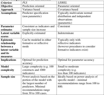
Table : Comparison of PLS and LISREL
Criterion PLS LISREL
Objective Prediction oriented Parameter oriented
Approach Variance based Covariance based
Assumptions Predictor specification (non parametric)
Typically multivariate normal distribution and independent observations
(parametric)
Parameter estimates
Consistent as indicators and sample size increase
Consistent
Latent variable scores
Explicitly estimated Indeterminate
Epistemic relationship between a latent variable and its
measures
Can be modeled in either formative or reflective mode
Typically only with reflective indicators
(however procedures to consider formative indicators exist)
Implications Optimal for prediction accuracy
Optimal for parameter accuracy
Model complexity
Large complexity (e.g. 100 constructs and 1000 indicators)
Small to moderate complexity (e.g.
less than 100 indicators)
Sample size Power analysis based on the portion of the model with the largest number of predictors. Minimal recommendations range from 30 to 100 cases.
Ideally based on power analysis of specific model – minimal
recommendations range from 100 to 800.
Source: Andreas Hammer (2006).
Empirical modeling strategy:
A two-stage exploratory-confirmatory method is for empirical modeling. The first-stage involves the following steps:
Step-I propose a theoretical model.
Step-II formulate the proposed model in the PLS framework for exploratory analysis. Step-III construct latent variable scores.
1) Select subgroups of individuals on the basis of the latent variable scores. These subgroups can be made on the basis of, for example, gender, region, age, resources, etc.
2) Rank individuals on the basis of the scores of one latent variable. 3) Correlate latent variable scores with the observed variables. 4) Estimate linear/non-linear relationships among latent variables. 5) Regress the observed variables on the latent variable scores.
The Theoretical Model:
The following simultaneous structural model is proposed. Capability is assumed to be a function of achieved functioning with process and opportunity freedom.
Capability = f (functioning, freedom) ---(1)
Functioning achievement is a function of conversion efficiency which is, in turn, a function of conversion factors (constraints) and resources.
Functioning = g(conversion efficiency) ---(2)
Conversion efficiency = h(constraints, resources)---(3)
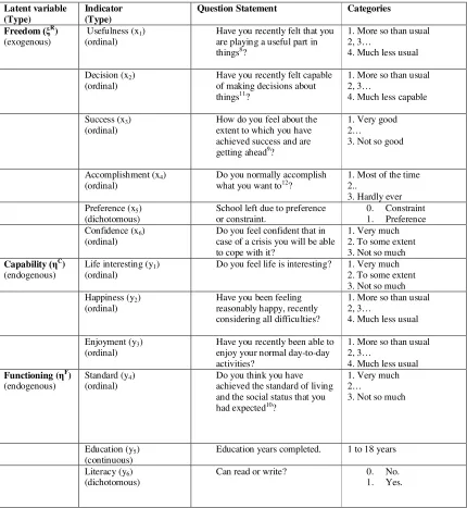
Table 1: Model variables and their indicators:
Latent variable (Type)
Indicator (Type)
Question Statement Categories
Freedom (ξR)
(exogenous)
Usefulness (x1)
(ordinal)
Have you recently felt that you are playing a useful part in things8?
1. More so than usual 2, 3…
4. Much less usual
Decision (x2)
(ordinal)
Have you recently felt capable of making decisions about things11?
1. More so than usual 2, 3…
4. Much less capable
Success (x3)
(ordinal)
How do you feel about the extent to which you have achieved success and are getting ahead9?
1. Very good 2…
3. Not so good
Accomplishment (x4)
(ordinal)
Do you normally accomplish what you want to12?
1. Most of the time 2..
3. Hardly ever Preference (x5)
(dichotomous)
School left due to preference or constraint.
0. Constraint 1. Preference Confidence (x6)
(ordinal)
Do you feel confident that in case of a crisis you will be able to cope with it?
1. Very much 2. To some extent 3. Not so much
Capability (ηC)
(endogenous)
Life interesting (y1)
(ordinal)
Do you feel life is interesting? 1. Very much 2. To some extent 3. Not so much Happiness (y2)
(ordinal)
Have you been feeling reasonably happy, recently considering all difficulties?
1. More so than usual 2, 3…
4. Much less usual
Enjoyment (y3)
(ordinal)
Have you recently been able to enjoy your normal day-to-day activities?
1. More so than usual 2, 3…
4. Much less usual
Functioning (ηF)
(endogenous)
Standard (y4)
(ordinal)
Do you think you have achieved the standard of living and the social status that you had expected10?
1. Very much 2…
3. Not so much
Education (y5)
(continuous)
Education years completed. 1 to 18 years
Literacy (y6)
(dichotomous)
Can read or write? 0. No. 1. Yes.
Note: The composite reliability indices for capability and freedom indicators are 0.8 and 0.6 respectively whereas it is low (0.3) for functioning indicators.
8
‘The process aspect, being concerned with the freedom of the person’s decisions, must take note of both (iia) the scope for autonomy in individual choices, and (iib) immunity from interference by others.’ (Sen, 2002).
9
‘[…..]opportunity-freedom cannot be sensibly judged merely in terms of possession of commodities, but must take note of the opportunity of doing things and achieving results one has reason to value.’(Sen, 2002).
10
Table:2 Causal Variables: Formative Indicators for conversion efficiency (ξE)
No. Variable Type Categories
1 Gender (x7) Categorical 1. Male
2. Female
2 Age (x8) Metric >30
3 Province (x9) Spatial 1. Punjab
2. Sind 3. Baluchistan 4. NWFP 4 Urban (x10) Spatial 1. Urban
2. Rural 5 Income (x11) Metric >0
6 Marital status (x12) Categorical 1. Never married
2. Currently married 3. Widow/Widower 4. Divorced 5. Separated
Note: The blue ellipses show exogenous variables and the green ellipses show endogenous variables in the inner or structural model. The outer or measurement model consists of reflexive and formative indicators.
Estimation of the model
(QML) method is applicable in the situation of non-normality yet it is not asymptotically efficient. The problems of identification and heteroscedasticity are checked before applying the 3SLS method.
Main Findings
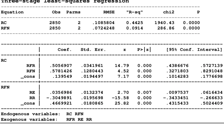
[image:21.595.86.454.351.555.2]The results show that income is associated with lower capability level which is consistent with the Anand and Hees (2006) finding. Moreover, conversion efficiency is positively related to functioning achievement. This result is in conformity with the Binder and Borekel (2008) result. Although it shows inefficient proportion of individuals yet it does not discriminate between voluntary and involuntary inefficient individuals. I have extended the concept of inefficiency into voluntary and involuntary inefficiency. According to mid efficiency criterion, there are 35% inefficient individuals. Out of these 35%, 36% are voluntary inefficient which are 22% of the total individuals in the sample. The capability is positively and significantly explained by the functioning achievement and the freedom which is consistent with Sen’s capability approach. The sign and size of coefficients are robust to various model specifications. The freedom and functioning have almost equal impact on the capability. The resources have greater but negative impact on functioning than relative efficiency (see Table 3).
Table 3
Three-stage least-squares regression
---
Equation Obs Parms RMSE "R-sq" chi2 P
---
RC 2850 2 .1085804 0.4425 1940.43 0.0000 RFN 2850 2 .0724248 0.0914 286.86 0.0000
---
--- | Coef. Std. Err. z P>|z| [95% Conf. Interval] ---+--- RC |
RFR | .5056907 .0341961 14.79 0.000 .4386676 .5727139 RFN | .5781426 .1280443 4.52 0.000 .3271803 .8291048 _cons | .139549 .0194497 7.17 0.000 .1014283 .1776698 ---+--- RFN |
RE | .0356986 .0132374 2.70 0.007 .0097537 .0616434 RR | -.3049891 .0195698 -15.58 0.000 -.3433451 -.266633 _cons | .4669921 .0180865 25.82 0.000 .4315433 .5024409 --- Endogenous variables: RC RFN
Exogenous variables: RFR RE RR
Table 4 shows inequality ratio of top decile average to bottom decile average for relative capability (RC), relative efficiency (RE), relative freedom (RFR), relative functioning (RFN), and relative resource (RR) ratios. The largest inequality is in the functioning achievement followed by capability and freedom. It is understandable since about 50% of the individuals in the sample are illiterate. The lowest inequality is in the resource distribution where top decile is getting 44% more resources than the bottom decile. There are no significant differences between provinces or urban and rural areas for these ratios.
Table 4
Inequality ratio
RC RE RFR RFN RR
[image:21.595.88.324.671.716.2]Conclusions and Policy Implications
The paper measures freedom aspect of capability by developing indicators from the survey data. The correctness of freedom measure depends on the quality of indicators and the robustness of statistical method. The paper also suggests criteria for the evaluation of empirical research within the capability approach framework.
The results show that capability is inversely related to resources and positively related to freedom and functioning. The computed relative capability and freedom inequality ratios are very high whereas relative functioning and efficiency inequality ratios are at a
moderate level. The conventional income inequality ratio is lower as compared to the capability dimensions ratios and close to the Gini-coefficient. The paper recommends the use of inequality measures instead of averaging measures particularly in developing countries where inequality levels are very high. The state-dependence due to human diversity calls for taking individual as a unit of analysis. The paper also recommends development of specific survey instruments in order to create better indicators for
capability dimensions and use of latent variable modeling for constructing latent variable scores, and their subsequent use in estimation. These findings suggest a capabilities-oriented public and education policies for the enhancement of knowledge dimension of capabilities in particular and human welfare in general. The focus of education policy should be extended from investment-oriented (human capital approach) to value-oriented (human capability approach).
References
Alkire, S. (2005). Measuring freedom aspects of capabilities.
_______. (2007). Measuring Agency: Issues and Possibilities. Indian Journal of Human Development, 1(1).
Anand, P., Hunter, G., Carter, I., Dowding, K., Guala, F., and Hees, M., (2005).The Measurement of Human Capabilities. www.oecd.org/dataoecd/63/37/38363699.pdf
Anand, P., and Hees, M. (2006).Capabilities and achievements: An empirical study, Journal of Socio-Economics, 35, 268-284.
Arif, G.M., Ali, M. S., Nasir, Z.M., Arshad, N. (2001).An Introduction to the 1998-99 Pakistan Socio-Economic Survey (PSES). MIMAP Technical paper series no. 4. Pakistan Institute of Development Economics, Islamabad, Pakistan.
Atkinson, A.B. (1999). The Contributions of Amartya Sen to Welfare Economics, Scandinavian Journal of Economics, 101(2). p.173-190.
Arrow, Kenneth. (1999).Amartya K. Sen’s Contributions to the Study of Social Welfare, Scandinavian Journal of Economics, 101(2).p.163-172.
Binder, M. and Broekel, T. (2008). Conversion Efficiency as a complementing measure of welfare in capability space.MPRA.
Bollen, Kenneth, A. (2002). Latent Variables in Psychology and the Social Sciences. Annual Review Psychology, 53, 605-34.
Bro, R. and Elden, L. (2009).PLS works. Journal of Chemometrics, 23 (2). 69-71.
Comim, F., Qizilbash, M., and Alkire, S. (ed.) (2008). The Capability Approach- Concepts, Measures, and Applications. Cambridge University Press.
Hammer, A. (2006). Enabling Successful Supply Chain Management –Coordination, Collaboration, and Integration for Competitive Advantage, Doctoral Thesis. University of Mannheim.
Huber, P., E. Ronchetti, and M.-P. Victoria-Feser (2004).Estimation of generalized latent trait models. Journal of the Royal Statistical Society, Series B 66, 893—908.
Jensen, U. (2000). Is it efficient to analyse efficiency rankings? Empirical Economics, 25: 189-208.
Kementa, J. (1991). Latent Variables in Econometrics. Statistica Neerlandica. 45(2). 73-84.
Kuklys, W. (2005). Amartya Sen’s Capability Approach-Theoretical Insights and Empirical Applications. Springer, Berlin et al.
Kumbhakar, S.C., and Lovell, C.A. (2000). Stochastic Frontier Analysis. CUP.
Olsson, Ulf. (1979). Maximum Likelihood Estimation of the Polychoric Correlation Coefficient. Psychometrika, 44 (4).
Pressman, S, and Summerfield, G. (2000). The Economic Contributions of Amartya Sen. Review of Political Economy, 12(1).
Robeyns, I. (2005). The Capability Approach: a theoretical survey. Journal of Human Development, 6(1): 93-117.
Ryan, R. M. and Deci, E. L. (2000).Self-Determination Theory and the Facilitation of Intrinsic Motivation, Social Development, and Well-Being. American Psychologist, January 2000.
Sen, A. K. (1987).The Standard of Living. CUP.
_________(2002). Rationality and Freedom, Cambridge, MA: Belknap. ________ (2001). Development as Freedom. Oxford University Press.
_________(1990). Justice: means versus freedoms. Philosophy and Public Affairs, 19(2).
________ (1992).Inequality reexamined, Oxford, OUP.
_________(1984).Resources, Values and Development, Oxford: Basil Blackwell.
_________(2004). Elements of a Theory of Human Rights. Philosophy and Public Affairs, 32(4).
_________(2002).Sen and Capabilities. Review of Political Economy, 14(4).
Appendix 1
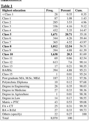
Table 1
Highest education Freq. Percent Cum.
< Class 1 28 0.35 0.35
Class 1 87 1.08 1.43
Class 2 285 3.53 4.96
Class 3 336 4.16 9.12
Class 4 432 5.35 14.47
Class 5 1,671 20.71 35.18
Class 6 344 4.26 39.44
Class 7 365 4.52 43.97
Class 8 1,012 12.54 56.51
Class 9 394 4.88 61.39
Class 10 1,638 20.3 81.69
Class 11 69 0.86 82.54
Class 12 613 7.6 90.14
Class 13 17 0.21 90.35
BA/BSc 394 4.88 95.23
Class 15 1 0.01 95.24
Post graduate MA, M.Sc, MEd. 187 2.32 97.56
Polytechnic Diploma 10 0.12 97.68
Degree in Engineering 28 0.35 98.03
Degree in Medicine 27 0.33 98.36
Degree in Agriculture 1 0.01 98.38
Degree in Law 14 0.17 98.55
Matric + PTC 43 0.53 99.08
FA + CT 25 0.31 99.39
BA + B.Ed 27 0.33 99.73
Others (specify) 22 0.27 100
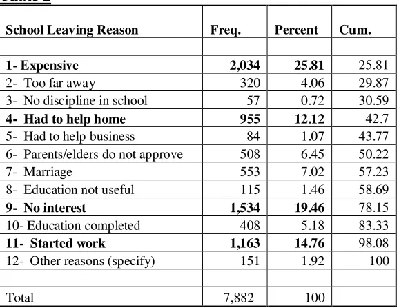
Table 2
School Leaving Reason
Freq. Percent Cum.
1- Expensive 2,034 25.81 25.81
2- Too far away 320 4.06 29.87
3- No discipline in school 57 0.72 30.59
4- Had to help home 955 12.12 42.7
5- Had to help business 84 1.07 43.77
6- Parents/elders do not approve 508 6.45 50.22
7- Marriage 553 7.02 57.23
8- Education not useful 115 1.46 58.69
9- No interest 1,534 19.46 78.15
10- Education completed 408 5.18 83.33
11- Started work 1,163 14.76 98.08
12- Other reasons (specify) 151 1.92 100
[image:26.595.88.377.115.338.2]
Total 7,882 100
Table 3
Subjective indicators for constraints and preferences:
Reason for leaving school
Constraint (c) or Preference (p)
1- Expensive C
2- Too far away C
3- No discipline in school C
4- Had to help home C
5- Had to help business C
6- Parents/elders do not approve C
7- Marriage C
8- Education not useful P
9- No interest P
10- Education completed P
11- Started work P
Table 4
School left due to Freq. Percent
constraint 1,015 52.73
preference 910 47.27
Total 1,925 100
Table 5
Literacy (can read
or write?) Freq. Percent
Yes 2,036 54.05
No 1,731 45.95
[image:26.595.89.377.342.709.2]Table 6
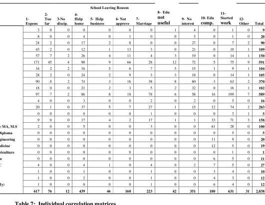
Highest School Leaving Reason
education
1- Expens
2-Too far
3-No discip.
4- Help home
5- Help business
6- Not approve
7-Marriage
8- Edu not useful
9- No interest
10- Edu comp.
11-Started work
12-
Other Total < Class 1 3 0 0 0 0 0 0 1 4 0 1 0 9
Class 1 8 0 0 4 0 1 0 0 5 0 1 0 20
Class 2 24 2 0 17 2 8 0 0 27 0 7 2 90 Class 3 45 2 0 12 1 13 3 0 21 0 10 1 109 Class 4 57 7 2 26 4 11 4 3 19 0 14 1 150 Class 5 171 45 4 90 9 66 28 12 72 5 75 9 591 Class 6 34 2 2 16 5 6 7 5 15 1 9 1 104 Class 7 28 2 0 24 2 9 3 3 18 0 14 1 105 Class 8 90 8 2 74 3 16 38 8 60 3 63 2 370 Class 9 18 0 0 21 2 3 5 2 32 0 16 1 102 Class 10 97 7 2 86 8 18 78 6 58 16 199 7 589
Class 11 4 0 0 3 0 0 2 0 2 0 5 0 16
Class 12 20 1 0 37 5 7 27 1 15 12 74 2 203
Class 13 0 0 0 0 0 0 1 0 0 0 3 1 5
BA/BSc 9 0 0 17 4 2 17 1 1 33 71 3 158 Post graduate MA, M.S 2 0 0 5 0 0 3 0 0 61 28 0 100 Polytechnic Diploma 0 0 0 0 0 0 0 0 0 0 5 0 5 Degree in Engineering 0 0 0 0 0 0 0 0 0 11 9 0 20 Degree in Medicine 0 0 0 0 0 0 0 0 0 12 5 0 19 Degree in Agriculture 0 0 0 0 0 0 0 0 0 0 1 0 1 Degree in Law 0 0 0 0 0 0 0 0 0 6 5 0 11 Matric + PTC 4 0 0 4 1 0 4 0 2 7 5 0 27
FA + CT 1 0 0 1 0 0 1 0 0 3 4 0 10
BA + B.Ed 1 0 0 2 0 0 1 0 0 4 3 0 12
[image:27.595.82.516.542.734.2]Others (specify) 1 0 0 0 0 0 1 0 0 6 4 0 12 Total 617 76 12 439 46 160 223 42 351 180 631 31 2,838
Table 7: Individual correlation matrices
Polychoric correlation matrix for reflexive indicators of freedom
s13Aq4 s13Aq5 s13Bq5 s13Bq6
s13Aq4 1
s13Aq5 .63066972 1
s13Bq5 .36165646 .3885846 1
s13Bq6 .35731299 .33248036 .6521731 1
Polychoric correlation matrix for formative indicators of conversion efficiency s1q2 s1q3a s1q6 prov ur lnincome s1q2 1
s1q3a -.29735372 1
s1q6 -.17683146 .6755722 1
prov -.01322384 -.04855938 -.09291133 1
ur -.17044364 -.0870671 .00282481 -.22736825 1
Polychoric correlation matrix for reflexive indicators of functioning
news2q3 s13Bq4 s13Aq4 s13Bq3
news2q3 1
s13Bq4 -.2019069 1
s13Aq4 -.15489569 .32239206 1
[image:28.595.89.513.329.428.2]s13Bq3 -.25200336 .57130337 .49267445 1
Table 8: Summary statistics Univariate Summary Statistics for Continuous Variables Variable Mean St. Dev. T-Value Skewness Kurtosis Minimum Freq. Maximum Freq. s1q3a 39.793 13.477 118.289 0.433 -0.178 10.000 1 87.000 2
news2q3 8.268 3.865 85.708 0.573 0.890 0.000 5 26.000 7
lnincome 10.455 1.000 418.741 -1.078 6.787 2.303 1 14.123 1
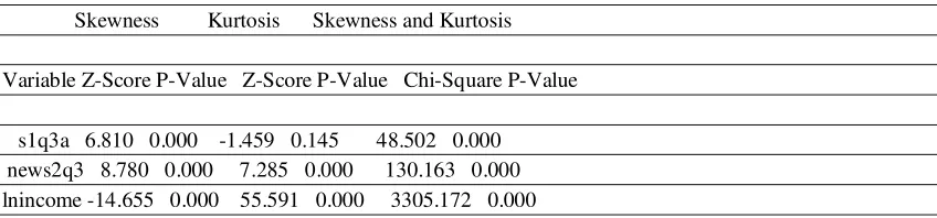
Test of Univariate Normality for Continuous Variables
Skewness Kurtosis Skewness and Kurtosis
Variable Z-Score P-Value Z-Score P-Value Chi-Square P-Value
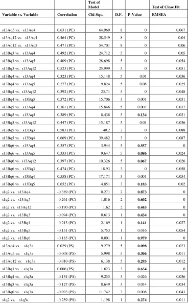
Table 9: Correlations and Test Statistics
(PE=Pearson Product Moment, PC=Polychoric, PS=Polyserial)
Test of
Model Test of Close Fit Variable vs. Variable Correlation Chi-Squ. D.F. P-Value RMSEA
s1q6 vs. s13Aq4 0.015 (PC) 13.96 11 0.235 0.013 s1q6 vs. s13Aq5 0.000 (PC) 28.423 11 0.003 0.031 s1q6 vs. s13Aq12 -0.004 (PC) 12.836 11 0.304 0.01 s1q6 vs. s13Bq3 0.017 (PC) 1.775 7 0.971 0 s1q6 vs. s13Bq4 -0.092 (PC) 5.845 7 0.558 0 s1q6 vs. s13Bq5 -0.082 (PC) 10.501 7 0.162 0.018 s1q6 vs. s13Bq6 -0.053 (PC) 11.742 7 0.109 0.021 s1q6 vs. s1q2 -0.176 (PC) 4.637 3 0.2 0.018 s1q6 vs. s1q3a 0.663 (PS) 187.616 7 0 0.127 prov vs. s13Aq4 -0.124 (PC) 26.891 8 0.001 0.038 prov vs. s13Aq5 -0.080 (PC) 49.708 8 0 0.057 prov vs. s13Aq12 -0.089 (PC) 34.532 8 0 0.046 prov vs. s13Bq3 -0.121 (PC) 10.318 5 0.067 0.026 prov vs. s13Bq4 0.025 (PC) 5.846 5 0.322 0.01 prov vs. s13Bq5 -0.017 (PC) 18.068 5 0.003 0.04 prov vs. s13Bq6 0.046 (PC) 32.946 5 0 0.059 prov vs. s1q2 -0.013 (PC) 2.339 2 0.311 0.01 prov vs. s1q3a -0.052 (PS) 10.457 5 0.063 0.026 prov vs. s1q6 -0.093 (PC) 13.312 11 0.273 0.011 ur vs. s13Aq4 0.006 (PC) 0.334 2 0.846 0 ur vs. s13Aq5 0.045 (PC) 1.117 2 0.572 0 ur vs. s13Aq12 0.108 (PC) 1.206 2 0.547 0 ur vs. s13Bq3 0.027 (PC) 8.576 1 0.003 0.069 ur vs. s13Bq4 0.016 (PC) 15.341 1 0 0.095 ur vs. s13Bq5 0.080 (PC) 5.84 1 0.016 0.055 ur vs. s13Bq6 0.076 (PC) 1.05 1 0.305 0.006 ur vs. s1q2 -0.169 (PC) 0 0 1 0.006 ur vs. s1q3a -0.090 (PS) 0.034 1 0.854 0 ur vs. s1q6 0.002 (PC) 2.39 3 0.496 0 ur vs. prov -0.229 (PC) 4.197 2 0.123 0.026 s13Aq4 vs. news2q3 -0.155 (PS) 4.36 5 0.499 0 s13Aq5 vs. news2q3 -0.129 (PS) 2.869 5 0.72 0 s13Aq12 vs. news2q3 -0.149 (PS) 11.675 5 0.04 0.029 s13Bq3 vs. news2q3 -0.252 (PS) 13.438 3 0.004 0.047 s13Bq4 vs. news2q3 -0.203 (PS) 3.881 3 0.275 0.014 s13Bq5 vs. news2q3 -0.259 (PS) 13.303 3 0.004 0.046 s13Bq6 vs. news2q3 -0.202 (PS) 6.126 3 0.106 0.026 s1q2 vs. news2q3 0.059 (PS) 0.046 1 0.831 0 news2q3 vs. s1q3a -0.025 (PE)
ur vs. news2q3 -0.279 (PS) 24.327 1 0 0.121 s13Aq4 vs. lnincome -0.230 (PS) 6.943 5 0.225 0.016 s13Aq5 vs. lnincome -0.194 (PS) 19.02 5 0.002 0.042 s13Aq12 vs. lnincome -0.196 (PS) 33.063 5 0 0.059 s13Bq3 vs. lnincome -0.245 (PS) 14.509 3 0.002 0.049 s13Bq4 vs. lnincome -0.233 (PS) 4.896 3 0.18 0.02 s13Bq5 vs. lnincome -0.291 (PS) 1.188 3 0.756 0 s13Bq6 vs. lnincome -0.255 (PS) 17.326 3 0.001 0.055 s1q2 vs. lnincome -0.291 (PS) 5.158 1 0.023 0.051 lnincome vs. s1q3a 0.096 (PE)
s1q6 vs. lnincome 0.139 (PS) 39.428 7 0 0.054 prov vs. lnincome 0.137 (PS) 55.861 5 0 0.08 ur vs. lnincome -0.298 (PS) 2.946 1 0.086 0.035 lnincome vs. news2q3 0.316 (PE)
Table 10: Correlation Matrix
s13Aq4 s13Aq5 s13Aq12 s13Bq3 s13Bq4 s13Bq5
s13Aq4 1
s13Aq5 0.631 1
s13Aq12 0.464 0.471 1
s13Bq3 0.492 0.409 0.523 1
s13Bq4 0.323 0.277 0.392 0.572 1
s13Bq5 0.361 0.389 0.447 0.583 0.669 1
s13Bq6 0.357 0.333 0.397 0.474 0.558 0.652
s1q2 -0.389 -0.261 -0.19 -0.094 -0.213 -0.151
s1q3a 0.029 -0.008 -0.01 0.006 -0.134 -0.127
s1q6 0.015 0 -0.004 0.017 -0.092 -0.082
prov -0.124 -0.08 -0.089 -0.121 0.025 -0.017
ur 0.006 0.045 0.108 0.027 0.016 0.08
news2q3 -0.155 -0.129 -0.149 -0.252 -0.203 -0.259
lnincome -0.23 -0.194 -0.196 -0.245 -0.233 -0.291
s13Bq6 s1q2 s1q3a s1q6 prov ur
s13Bq6 1
s1q2 -0.185 1
s1q3a -0.093 -0.259 1
s1q6 -0.053 -0.176 0.663 1
prov 0.046 -0.013 -0.052 -0.093 1
ur 0.076 -0.169 -0.09 0.002 -0.229 1
news2q3 -0.202 0.059 -0.025 -0.067 0.088 -0.279
lnincome -0.255 -0.291 0.096 0.139 0.137 -0.298
news2q3 lnincome
news2q3 1
lnincome 0.316 1
Appendix 2
PLS Algorithm (Bro and Elden, 2009)
T j i i i
i T i i
i T i
i T i i
T i T i i
p t X X
t X p
w x
w x t
y x
y x w
k i
X X
1 1 1 1 1 1 0
(d)
(c)
|| ||
(b)
|| || (a)
. ,..., 2 , 1 For . 2