http://dx.doi.org/10.4236/cs.2016.710254
ODFF: Optimized Dual Fuzzy Flow
Controller Based Voltage Sag
Compensation for SMES-Based
DVR in Power Quality
Applications
M. Manikandan
1, A. Mahabub Basha
21Department of Electrical and Electronics Engineering, Erode Sengunthar Engineering College, Thudupathi, India
2Department of Electronics and Communication Engineering, K.S.R. College of Engineering, Erode, India
Received 3 May 2016; accepted 15 May 2016; published 16 August 2016
Copyright © 2016 by authors and Scientific Research Publishing Inc.
This work is licensed under the Creative Commons Attribution International License (CC BY). http://creativecommons.org/licenses/by/4.0/
Abstract
The booming electronics itself carries an impact on power quality. Superconducting Magnetic En-ergy Storage (SMES) is proposed to enhance power quality in three-phase systems under various loads. This paper aimed to compensate the voltage sags under various faults in the grid systems. The SMES is selected as an energy storage unit to improve the capability of voltage sag compensa-tion. Optimized Dual Fuzzy Flow (ODFF) logic controller is designed to prevent the voltage sag time during excessive phase voltage variation. Hence the proposed controller strategy reduces the total harmonic distortion during various fault conditions. To regulate the contribution of active power, the least possible value is improved using ODFF. The depth of voltage sags compensation is achieved by the over modulation and an iterative loop is designed in the control block. While pro-tecting sensitive loads from voltage disturbances, and sags initiated by the power system, the proposed configuration is advantageous for an industrial implementation. It is found that the proposed method can result in more than 50% additional sag support time when compared with the previous methods such as PI and PSO. Utilizing MATLAB Simulink, compensation of sag and minimization of THD is established, and the simulation tests are performed to evaluate the per-formance of the proposed control method.
Keywords
1. Introduction
In industrial distribution systems, the grid voltage disturbances (voltage sags, swells, flicker, and harmonics) are the most common power quality problems. Sag, being the most frequent voltage disturbance, is typically caused by a fault at the remote bus and is always accompanied by a phase angle jump. The phase jump in the voltage can initiate transient current in the capacitors, transformers, and motors [1].
Harmonics and non-linear loads lead to major power quality issues. The Dynamic Voltage Restorer (DVR) in [2], nevertheless uniquely compensates on sag, it limits itself for certain percentage and thus the quality problem is not suppressed completely. The sag compensation factor is directly proportional to the rate of sag depth in a grid system. The Dynamic Voltage Restorer with other controlling techniques gives positive result on quality enhancement with its advantage of less computational efforts and low cost [3].
The Superconducting Magnetic Energy Storage (SMES) [4] is expected to contribute to high power quality due to its characteristics of swift response and energy storage. The system voltage wavering can be compensated by the SMES. The parallel connection of SMES controls the system voltage indirectly by regulating the inject-ing current of SMES. The SMES can be expressed as
2
1 d d
2 d d
e i
E LI P LI VI
t t
= = = = (1)
The capability of compensation is inclined by short circuit capacity of the system and SMES location. The power factor is another crucial factor to be noted for analyses.
The DVR based SMES leads to better compensation than individual performance of DVR. The series injected voltage of the DVR can be written as
inj load s
V =V +V (2)
Voltage sag is a momentary decrease in RMS AC voltage 0.1 - 0.9 p.u of the nominal voltage at the power frequency derived in [5]. Voltage swell or sag (dips) is caused by faults occurring in the customers’ installations on the public distribution systems. The power quality problems become major concerns of industries due to massive loss of time and cost. Reduction of voltage sags, harmonic distortion and interruptions solves the issues in power quality problems. The number of methods available to overcome the voltage sags such as DVR is one of the best methods to compensate voltage sag. DVR is an electronic device that is able to compensate the volt-age sag on critical loads dynamically. Thus the compensation of sag is done by fuzzy logic and BFO fuzzy logic function which takes two inputs: error (e) and error rate and gives one output.
In this paper, section 2 describes the brief survey on the related work and section 3 presents the proposed me-thodology and Optimized Dual Fuzzy Flow (ODFF) logic controller circuits are briefed in section 4 and section 5. The simulation test outputs are discussed in section 6 and finally concluded in section 7.
2. Previous Research
Numerous related research works are already existed in literature which based on power quality control, THD and Voltage sag compensation system. Some of them are reviewed here.
The emphasis is on either reducing the voltage rating of DVR by aligning the injected voltage with the source voltage (i.e., in-phase compensation) or minimizing the dc storage capacity by using the reactive power com-pensation/energy-optimized approach presented in [6]. All of these methods, however, cannot correct the phase jump and thus can result in premature tripping of sensitive loads discussed in [7].
Kumar and Mishra discussed about the first category are series active filters (SeAFs), including hybrid- type ones [8]. They were developed to eliminate current harmonics produced by nonlinear load from the power sys-tem. SeAFs are less scattered than the shunt type of active filters presented in [9]. The advantage of the SeAF compared to these hunt type is the inferior rating of the compensator versus the load nominal rating. However, the complexity of the configuration and necessity of an isolation series transformer had decelerated their indus-trial application in the distribution system are briefed in [10].
power distortions at the point of common coupling (PCC). Hypothetically, they are capable of compensating current harmonics, ensuring a Power Factor (PF) correction at the PCC [12]. The concept of Decoupled State Feedback Control for Current Source Power Conditioning is presented in [13].The idea of compensating voltage fluctuations using SMES based Dynamic Voltage Restorer for long term where the simulation result illustrates the superconducting magnets increases the compensation when compared to the capacitor banks [14].
The fuzzy system has proved the better minimization of the THD than using PI controllers. The output depicts that the THD is minimized after the BFO optimization. DVR based different controllers are designed to improve power quality regarding sag and swell characteristics under different load conditions [15]. M. Manikandan and A. Mahabub Basha proposed their work on the improvement of power quality and three phase or single phase fault leading to sag compensation by SMES combined with Fuzzy logic control [16].
The basic concept of fuzzy control strategy and problem-solving methods are discussed with clear key points [17]. The application of fuzzy logic to knowledge representation relating to the industrial computational system is presented in [18]. The concept of uncertainty and imprecision in the context of knowledge, meaning, and in-ference is discussed.
3. Proposed Topology
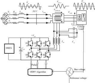
The schematic diagram of the proposed topology with detailed phase sag supporter is shown in Figure 1. The voltage sag supporter is provided between the PCC and the load. When a voltage sag occurs at the PCC of any of the phases, the corresponding sag supporter injects appropriate voltage in series with the supply voltage to maintain the desired load voltage.
[image:3.595.150.469.415.692.2]To account for phase Skip compensation, this topology incorporates the merits of the inter phase ac–ac to-pology, by having a sag supporter with two choppers and isolation transformers in each phase. The secondary’s of the isolation transformers are connected such that they add the output voltages of the choppers and inject them. Deriving the injected voltage from two voltage sources facilitates the realization of the desired reference voltage with phase shift. In this scheme, compensation of fundamental quantities has been considered. In case of harmonics; fundamental components are extracted and compensated by the scheme.
3.1. Proposed Phase Skip Scheme for Voltage Sag Compensation
The work presented in this paper proposes an enhanced voltage sag compensation method to extend the SMES based DVR compensation time. It optimizes the gradient of the dc link voltage (dvdc/dt) by regulating the amount of active power injected by SMES based DVR. In the proposed method, the controller restores both phase and amplitude of the load voltage to the presag value and then initiates a transition toward the Low active power (LAP) mode. The overall operation sequence and implementation of the proposed compensation method is discussed in the following subsections.
3.1.1. Phase Skip Detection and Presag Restoration
For detecting the phase Skip, two PLLs are employed (one over the load voltage and another over the source voltage), giving θVLand θVg, respectively. As soon as the sag is detected, the first step is to determine the SMES based DVR initial injection angle that avoids the phase Skip at the load side. This is done by freezing the load voltage PLL that gives the presag angle (θVLp). On the other hand, the unrestricted grid voltage PLL gives the grid voltage phase (θVg). The difference between these two angles gives the initial angle of injection Note that, in the steady state, both angles will be identical, and thus, the difference will be zero. For sag detection, the abso-lute difference between the reference load voltage (1 p.u.) and the actual grid voltage (p.u.) in synchronous ref-erence frame is calculated as follows:
(
)
L
init θ VLP Vg L
θ = + θ −θ =θ +δ (3)
For sag detection, the absolute difference between the reference load voltage (1 p.u.) and the actual grid volt-age (p.u.) in synchronous reference frame is calculated as follows
2 2
1
sag gd gq
V V V
∆ = − + (4)
3.1.2. Controlled Transition toward the LAP Mode
Once the presag voltage is successfully restored, after one cycle, a smooth transition toward the LAP mode is initiated and completed over the next one to two cycles. The final injection angle of SMES based DVR (θfin) is given as ( ) ( ) ( ) 1 cos sin 1 1 cos π if 2
π tan if
L L L L Vg sag fin L sag LCOS V V V V θ θ θ θ γ θ ′ − ≤ − − > − + ∆ − ∆ = (5)
The first part of Equation (5) represents the self-supporting mode of operation in which the SMES based DVR absorbs active power (relatively very small amount) from the grid to overcome the system losses and thus main-tains a constant voltage across the dc link capacitor. The term γ indicates the reduction in θfin due to loss com-ponent and it is determined by the dc link (PI) controller. The second part of Equation (5) represents a case where the self-supported dc link. To ensure a smooth changeover, a transition ramp is defined between the initial and final operating points, as given in the following:
fin init trans init
T
θ θ
θ =θ + −
∆ (6)
3.1.3. Iterative Decrement in Injection Angle
In self-supporting mode, the SMES based DVR can compensate the sag for an indefinitely long time. However, for deeper sag depths, there is certain nonzero active power injected by SMES based DVR. This causes a reduc-tion in the energy stored in the dc link capacitor, and consequently, its voltage reduces (gradually). To maintain the required voltage at the inverter output side, the controller increases the modulation index mi until it reaches
control loop is used, which constantly monitors the dc link voltage and decreases θfin in Equation (6) to keep Vdc>
Vdc−min and is given as
fin fin
θ =θ − (7)
3.1.4. Operation Sequence
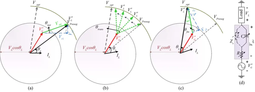
Figures 2(a)-(c) depict the overall operation sequence of the proposed phase Skip compensation scheme. The transition from high active power mode (presag) to LAP mode is shown in three steps. The illustration is for the case where the sag depth is more than the limit in (5) and there is a positive phase Skip associated with the sag. As discussed previously and shown in Figure 2(a), SMES based DVR initiates the compensation by supplying high active power to the load (Vr1_ Vx1) and restores both magnitude and phase of the load voltage to presag
values. After one cycle, the transition toward the LAP mode is initiated, and SMES BASED DVR gradually in-creases the contribution of reactive power. As seen from Figure 2(b) and Figure 2(c), the injected voltage mag-nitude and its phase angle are gradually increasing until VLreaches VL−opt. Note that at the final operating point
Vr1_ Vx1. The aforementioned SMES based DVR operation can be viewed as an equivalent variable impedance
Zv where the operation begins with dominant resistive impedance Zv= R (high active power) and completes as dominant capacitive impedance Zν≈ XC (high reactive power).
4. SMES Based DVR ODFF Switching Logic
Selection of switching logic for the proposed topology to compensate voltage sags are elucidate in this section. To obtain the reference load voltage, the control system is divided into two sub modules: 1) phase Skip detection plus SMES based DVR injection angle calculation and 2) LAP injection.
To achieve a decoupled active and reactive power control, the phase of the line current is considered as the reference and is obtained by the PLL. The phase Skip detection block computes the SMES based DVR initial (presag injection) angle and final (LAP injection) angle. As shown in Figure 3, the obtained SMES based DVR reference voltage Vdvr is compared with the actual voltage in the stationary reference frame. A propor-tional-resonant (PR) controller with a large gain at the grid fundamental frequency is used for accurate tracking of Vdvr. To compensate for SMES based DVR system losses, Vdvr is added as a feed forward signal to the output of the PR controller. The dc link voltage is constantly monitored in an iterative control loop to regulate the in-jected voltage angle, thus avoiding over modulation. Note that this block is only required when the sag depth is close to the system design limit.
4.1. Proposed ODFF Optimized Dual Fuzzy Flow Algorithm
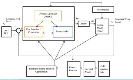
[image:5.595.90.534.515.676.2]The proposed ODFF flow is represented in Figure 4. The proposed system is designed to consider Fault distur-
Figure 3. Detailed block diagram of the proposed phase Skip compensate on method with LAP injection. (Cited from Power Electronics Converters, Applications and Design (Wiley, 2003)).
Figure 4. Proposed ODFF fuzzy controller.
bances of the DVR. Initially, Continuous Wavelet Transform is applied to extract the features of Power system dataset block. The difference in generated and converter voltage is identified. The proposed Fuzzy uses two models. The first model is called the plant, which describes a virtual Machine model. The second type of model is known as a system model, which shows the load voltage regulatory system in a SMES based DVR model. The Proposed model is used to specify the AC load assessment whenever sags are generated, and LAP mode is in-jected subcutaneously. And also this model finds a suitable way of directing voltage injections.
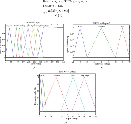
( )
[image:6.595.95.535.339.606.2]where x and y are the input variables, A and B represents fuzzy sets in the antecedent part, and the consequent part (output) is z= f x y
( )
, which is a crisp function, e.g.( )
x y, =p x0 +p y1 +r. This equation represents first-order polynomial function, but it can also be any function that describes the output within the fuzzy region mentioned by the antecedence of the rule. There are two unknowns design parameters: p0 and p1, the value forthese parameters are identified through a linear system of algebraic equations (Figure 5). The degree the input matches ith rule is typically computed using min operator:
( )
( )
(
)
min , , 1, 2, and 1, 2
i Aj Bk
w = µ x µ y j= k= (9)
Each specified fuzzy rule has a crisp output. The Overall output is attained through weighted average (reduce computation time of defuzzification required in a Mamdani model)
1 1 2 2 1 2
w z w z z
w w
+ =
+ (10)
where wi is matching degree of rule Ri (result of the if … part evaluation), i = 1, 2. The solution for the coeffi-cients of the consequent in TSK Systems
( )
( )
[
]
( )
1
1 0 1
1 0 1
1
Rule : is THEN
COMPOSITION
*
x x y p p x
x p p x
y x µ µ µ = + + =
0 50 100 150 200 250 300 350 400 450 500 0 0.2 0.4 0.6 0.8 1 Input voltage D eg ree o f m em b er sh ip
Very Low Low NormalHigh High2 High3Very High1Very High2
TMF Plot of Input - 1
-20 -15 -10 -5 0 5 10 15 20
0 0.2 0.4 0.6 0.8 1 Reference Voltage D eg re e o f m em b er sh ip
Low Normal High
TMF Plot of Input -2
(a) (b)
0 5 10 15 20 25 30 35 40 45 50 0 0.2 0.4 0.6 0.8 1 Output Voltage D eg re e o f m em b er sh ip
Very Low Normal High Very High TMF Plot of Output
(c)
[image:7.595.91.535.276.696.2]There are two unknowns: p0 and p1. So we need two simultaneous equations for two values of x, say x1 and x2,
and two values of y – y1 and y2
1 0 1 1
2 0 1 2
1 2 1 1 2 1 2 0 1 1 2 ;
y p p x
y p p x
y y p x x y y p y x x = + = + − = − − = − −
In order to determine the values of the parameters p in the consequents, one solves the LINEAR system of al-gebraic equations and tries to minimize the difference between the ACTUAL output of the system (Y) and the simulation [X]T[P]:
[ ] [ ] [ ]
TY − X P ≤ε
4.1.1. Algorithm Flow of ODFF
[image:8.595.86.540.656.723.2]• FUZZUFICATION: The values of the membership functions for the two values x1 = 12 & x2 = 5 shown in
Table 1.
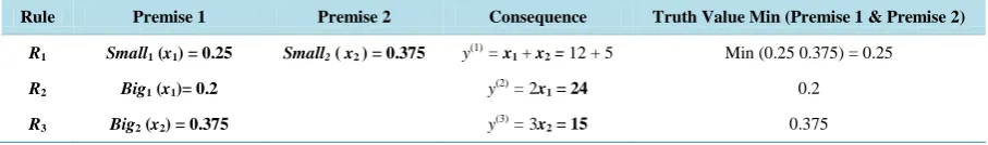
• INFERENCE & CONSEQUENCE: The Sample System Rules are shown in Table 2.
• AGGREGATION:
(
)
1 12 & 2 5
*
i i i
x x
y S y y y S y y
= =
= = =
Using a Centre of Area computation for y we get:
( ) ( )
( )
1,3 1,3
*
0.25 17 0.2 24 0.375 15 17.8 0.25 0.2 0.375
i i i
i i
y y y
y y y y = = = = = × + × + × = = + +
∑
∑
4.1.2. Optimization of ODFF Parameter Tuning
The simulation of system is based on the intensity of pheromone and the path length. The probability with which an ant ‘a’ selects the path from i to j is defined in Equation,
Table 1. Sample system values: two values x1 = 12 & x2 = 5 (Cited from industrial
applications of fuzzy control (Sugeno M., 1985)).
Small1 Small2 Big1 Big2
x1 12 0.25 0 0.2 1
x2 5 0.6875 0.375 0 0.375
Table 2. Sample system rules (cited from industrial applications of fuzzy control. (Sugeno M., 1985)).
Rule Premise 1 Premise 2 Consequence Truth ValueMin (Premise 1 & Premise 2)
R1 Small1 (x1) = 0.25 Small2 ( x2 ) = 0.375 y(1)=x1 + x2= 12 + 5 Min (0.25 0.375) = 0.25 R2 Big1 (x1)= 0.2 y(2)= 2x1=24 0.2
( )
( )
( ) (
(
)
)
1 2
2 1
1
, if , 1
0, Otherwise d i
ij ij d
i d
ij il il
l M
t L
j M
p t t L
γ γ γ γ τ τ ∈ ∈ =
∑
(11)where τij and Lij are the intensity of pheromone and the length of the path between features j and i, respec-tively.
γ
1 andγ
2 are the control parameters for defining the weight of the trail intensity and the length of thepath, respectively.
M
ia is the set of neighbors of feature i for the dth ant. After selecting the next path of fea-tures, the trail intensity of pheromone is updated and defined in Equation (12).( )
1 , if , ,( )
global-best-tour 0, Otherwiseij
i j
t Lr
τ ∈
∆ =
(12)
0< ≤ρ 1 is the phenomenon trial evaporation rate. ∆τij is the amount of pheromone trail added to τij by ants. d is a constant parameter. Lr is the length of the global best tour.
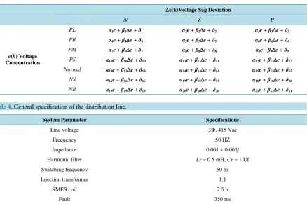
Table 3 expresses rules like:
Rule 1: If e(k) is PL AND ∆e(k) is N then ∆u(k) = α1e + β1∆e + δ1
Rule 2: If e(k) is PL AND ∆e(k) is Z then ∆u(k) = α2e + β2∆e + δ2 ··· etc …
Rule 21: If e(k) is NB AND ∆e(k) is P then ∆u(k) = α21e + β21∆e + δ21
α, β and δ are design parameters whose values are determined by the fuzzy system developer, based on relat-ing the behaviour of the errors and change in errors over a fixed range of changes in control. There are 2N a total of design parameters for rules. These TSK parameters are selected by the trial and error method.
5. Results and Discussions
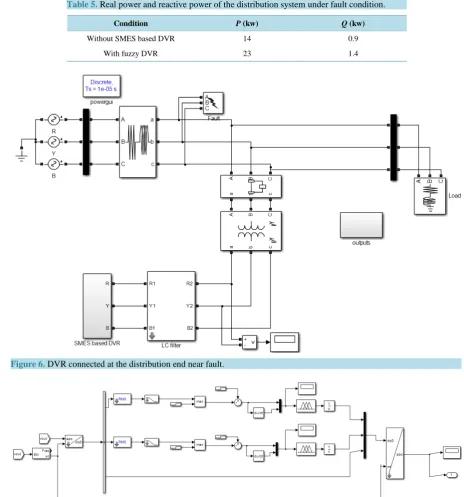
The specifications of the fault occurring system is specified with all the fundamental parameters in Table 4. The values of real power and reactive power at the generation side during fault condition in Table 5.
Table 3. Proposed fuzzy controller rules (Cited from Industrial applications of fuzzy control (Sugeno M., 1985)).
∆e(k)Voltage Sag Deviation
N Z P
e(k) Voltage
Concentration
PL α1e + β1∆e + δ1 α2e + β2∆e + δ2 α3e + β3∆e + δ3
PB α4e + β4∆e + δ4 α5e + β5∆e + δ5 α6e + β6∆e + δ6
PM α7e + β7∆e + δ7 α8e + β8∆e + δ8 α9e +β9∆e + δ9
PS α10e + β10∆e + δ10 α11e + β11∆e + δ11 α12e + β12∆e + δ12
Normal α13e + β13∆e + δ13 α14e + β14∆e + δ14 α15e + β15∆e + δ15
NS α16e + β16∆e + δ16 α17e + β17∆e + δ17 α18e + β18∆e + δ18
[image:9.595.100.539.429.720.2]NB α19e + β19∆e + δ19 α20e + β20∆e + δ20 α21e + β21∆e + δ21
Table 4. General specification of the distribution line.
System Parameter Specifications
Line voltage 3Φ, 415 Vac
Frequency 50 HZ
Impedance 0.001 + 0.005j
Harmonic filter Lr = 0.5 mH, Cr = 1 Uf
Switching frequency 50 hz
Injection transformer 1:1
SMES coil 7.5 h
Table 5. Real power and reactive power of the distribution system under fault condition.
Condition P (kw) Q (kw)
Without SMES based DVR 14 0.9
With fuzzy DVR 23 1.4
[image:10.595.92.537.471.589.2]Figure 6. DVR connected at the distribution end near fault.
Figure 7. Feedback comparator block (Cited from Knowledge representation in fuzzy logic. (Zadeh, L.A., 1989)).
The SMES based Dynamic Voltage Restorer circuit in the distribution system is shown below in Figure 6. The control block of chopper circuit is shown in Figure 7 which eliminates the harmonic contents in the phase voltage. This SMES based DVR gets the input from the PWM inverter that which gives the control signal for compensation. The control block shown above receives the parameters by conversion process of abc/dq transform during fault condition and compares with the reference value that which is fed to the SMES based DVR block. The error is filtered not just by comparing the dq values but with the defalut value set to the error comparator block.
Figure 8. Fuzzy logic control references (Cited from Fuzzy logic Toolbox MATLAB. (2013 a)).
ranges from −0.5 to +0.5.
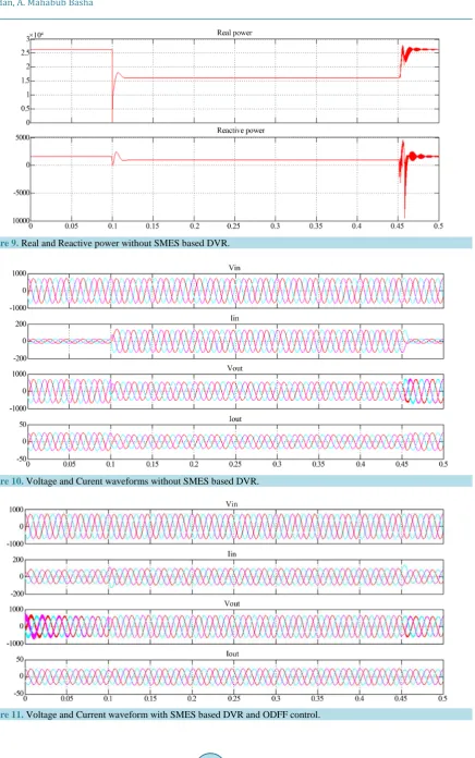
The real and reactive power of the three phase distribution line under fault condition whose duration is from 0.1 sec to 0.45 sec without any control techniques is shown in Figure 9. Figure 10 shows the input and output current and voltage waveform during current and voltage waveform at fault without SMES based DVR. In the same manner Figure 11 shows the real and reactive power of the three phase distribution line under fault condi-tion using ODFF control techniques is shown in Figure 12. Shows the input and output current and Voltage waveform during current and voltage waveform at fault using SMES based DVR.
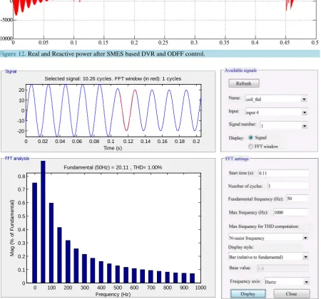
Figure 13 shows the total harmonic distortion value at fault condition before SMES based DVR control the
value reaches for about 1.00% for 50 Hz while in the case of using proposed control technique produces very less Distortion value of 0.12% for 50 HZ shown in Figure 14. THD is the summation of all harmonic compo-nents of the voltage or current waveform compared against the fundamental component of the voltage current wave. THD can exceed 1 and generally expressed as a percentage. THD calculated as
(
2 2 2 2)
2 3 4
1
THD n 100%
V V V V
V
+ + + +
= + (13)
The Total Harmonic Distortion THD value after fault compensation primarily sag compensation is shown above in Figure 14 where the range has reduced to 0.12% for 50 Hz.
The cosine of angle between the voltage and current is known as power factor (pf)
active power power factor
apparent power
= (14)
The power factor for the 3 phase system with the ODFF controller for the sag compensation has been ob-tained as 0.94.
Figure 15 and Figure 16 show the comparative results of with and without using SMES based DVR-ODFF
Figure 9. Real and Reactive power without SMES based DVR.
Figure 10. Voltage and Curent waveforms without SMES based DVR.
[image:12.595.108.520.83.278.2]Figure 12. Real and Reactive power after SMES based DVR and ODFF control.
Figure 13. THD without using ODFF control.
controller are shown in Figure 17.
6. Conclusion
The compensation on sag in three phase system at distribution end, when eliminated, enhances the stability of
0 0.02 0.04 0.06 0.08 0.1 0.12 0.14 0.16 0.18 0.2 -20
-10 0 10 20
Selected signal: 10.26 cycles. FFT window (in red): 1 cycles
Time (s)
0 100 200 300 400 500 600 700 800 900 1000 0
0.1 0.2 0.3 0.4 0.5 0.6 0.7 0.8
Frequency (Hz)
Fundamental (50Hz) = 20.11 , THD= 1.00%
M
ag (
%
of
F
undam
ent
al
[image:13.595.89.540.216.636.2]Figure 14. THD Results using proposed ODFF control.
[image:14.595.171.468.432.554.2]
Figure 15. THD comparison of ( without & with) SMES based DVR in ODFF controller.
0.88 0.9 0.92 0.94 0.96
Po
w
er
fa
ct
or
Time in sec
POWER FACTOR IMPROVEMENT IN WITHOUT DVR AND WITH DVR
without DVR with DVR
Figure 16. Power factor improvement in (with & without) SMES based DVR in ODFF controller.
0 0.05 0.1 0.15 0.2 0.25
-20 -10 0 10 20
Selected signal: 14.75 cycles. FFT window (in red): 1 cycles
Time (s)
0 100 200 300 400 500 600 700 800 900 1000 0
0.01 0.02 0.03 0.04 0.05 0.06 0.07
Frequency (Hz)
Fundamental (50Hz) = 24.01 , THD= 0.12%
M
ag (
%
of
F
undam
ent
al
[image:14.595.185.444.597.704.2]0 0.2 0.4 0.6 0.8 1 1.2 1.4
PI PSO ODFF
TH
D (
%
)
THD with controller
[image:15.595.171.461.88.227.2]THD with controller
Figure 17. Comparison of THD with many different controllers.
the supply power and also the sustained of the power factor without variation as it is tightly coupled to THD where the results imply the betterment on THD value reduction when compared with the SMES based DVR control without the combination of SMES coil and dual fuzzy logic control.
References
[1] Paliwal, M., Verma, R.C. and Rastogi, S. (2014) Voltage Sag Compensation Using Dynamic Voltage Restorer. Ad-vances in Electronic and Electrical Engineering, 4, 645-654.
[2] Sharanya, M., Basavaraja, B. and Sasikala, M. (2012) An Overview of Dynamic Voltage Restorer for Voltage Profile Improvement. International Journal of Engineering and Advanced Technology, 2, 127-135.
[3] Shi, J., Tang, Y.J., Yang, K., Chen, L., Ren, L. and Cheng, S.J. (2010) SMES Based Dynamic Voltage Restorer for Voltage Fluctuations Compensation. IEEE Transactions on Applied Superconductivity, 20, 3120-3130.
[4] Bollen, M.H.J. (2000) Understanding Power Quality Problems. IEEE Press, New York.
[5] Nielsen, J.G., Blaabjerg, F. and Mohan, N. (2001) Control Strategies for Dynamic Voltage Restorer, Compensating Voltage Sags with Phase Jump. Proceedings of the 16th Annual IEEE Applied Power Electronics Conference and Ex-position, Anaheim, August 2001, 1267-1273. http://dx.doi.org/10.1109/apec.2001.912528
[6] Kanjiya, P., Singh, B., Chandra, A. and Al-Haddad, K. (2013) “SRF Theory Revisited” to Control Self-Supported Dy-namic Voltage Restorer (DVR) for Unbalanced and Nonlinear Loads. IEEE Transactions on Industrial Applications, 49, 2330-2340. http://dx.doi.org/10.1109/TIA.2013.2261273
[7] Wessels, C., Gebhardt, F. and Fuchs, F.W. (2011) Fault Ride-Through of a DFIG Wind Turbine Using a Dynamic Voltage Restorer during Symmetrical and Asymmetrical Grid Faults. IEEE Transactions on Power Electronics, 26, 807-815. http://dx.doi.org/10.1109/TPEL.2010.2099133
[8] Kumar, C. and Mishra, M. (2014) A Multifunctional DSTATCOM Operating under Stiff Source. IEEE Transactions on Industrial Electronics, 61, 3131-3136. http://dx.doi.org/10.1109/TIE.2013.2276778
[9] Li, Y.W., Vilathgamuwa, D.M., Blaabjerg, F. and Loh, P.C. (2007) A Robust Control Scheme for Medium-Vol- tage-Level DVR Implementation. IEEE Transactions on Industrial Electronics, 54, 2249-2261.
http://dx.doi.org/10.1109/TIE.2007.894771
[10] Sadigh, A.K. and Smedley, K.M. (2012) Review of Voltage Compensation Methods in Dynamic Voltage Restorer (DVR). Proceedings of the IEEE Power and Energy Society General Meeting, San Diego, 22-26 July 2012, 1-8. http://dx.doi.org/10.1109/pesgm.2012.6345153
[11] Du, S.X., Liu, J.J. and Lin, J.L. (2013) Hybrid Cascaded H-Bridge Converter for Harmonic Current Compensation.
IEEE Transactions on Power Electronics, 28, 2170-2179. http://dx.doi.org/10.1109/TPEL.2012.2216550
[12] Javadi, A., Fortin Blanchette, H. and Al-Haddad, K. (2012) A Novel Transformerless Hybrid Series Active Filter.
Proceedings of the 38thAnnual International Conference and Exposition of the IEE EIECON, Montreal, 25-28 Octo-ber 2012, 5312-5317. http://dx.doi.org/10.1109/iecon.2012.6389536
[13] Shi, J., Tang, Y.J., Ren, L., Li, J.D. and Cheng, S.J. (2008) Discretization-Based Decoupled State Feedback Control for Current Source Power Conditioning System. IEEE Transactions On Power Delivery, 23, 2097-2104.
[15] Manikandan, M. and Mahabub Basha, A. (2013) Power Quality Compensation Using SMES Coil with FLC. Interna-tional Journal of Advances in Engineering & Technology, 6, 1855-1868.
[16] Jang, J.-S.R. and Sun, C.-T. (1997) Neuro-Fuzzy and Soft Computing: A Computational Approach to Learning and Machine Intelligence. Prentice Hall, Upper Saddle River.
[17] Sugeno, M. (1985) Industrial Applications of Fuzzy Control. Elsevier Science Pub. Co., Japan.
[18] Zadeh, L.A. (1989) Knowledge Representation in Fuzzy Logic. IEEE Transactions on Knowledge and Data Engineer-ing, 1, 89-100. http://dx.doi.org/10.1109/69.43406
Submit or recommend next manuscript to SCIRP and we will provide best service for you:
Accepting pre-submission inquiries through Email, Facebook, LinkedIn, Twitter, etc. A wide selection of journals (inclusive of 9 subjects, more than 200 journals) Providing 24-hour high-quality service
User-friendly online submission system Fair and swift peer-review system
Efficient typesetting and proofreading procedure
Display of the result of downloads and visits, as well as the number of cited articles Maximum dissemination of your research work