Single and multiple object tracking using a multi feature joint sparse representation

BIROn - Birkbeck Institutional Research Online

Hu, W. and Li, W. and Zhang, X. and Maybank, Stephen J. (2014) Single

and multiple object tracking using a multi-feature joint sparse representation.

IEEE Transactions on Pattern Analysis and Machine Intelligence 37 (4), pp.

816-833. ISSN 0162-8828.

Downloaded from:

Usage Guidelines:

Please refer to usage guidelines at or alternatively

Single and Multiple Object Tracking Using a Multi-Feature

Joint Sparse Representation

Weiming Hu, Wei Li, and Xiaoqin Zhang

(National Laboratory of Pattern Recognition, Institute of Automation, Chinese Academy of Sciences, Beijing 100190) {wmhu, weili, xqzhang}@nlpr.ia.ac.cn

Stephen Maybank

(Department of Computer Science and Information Systems, Birkbeck College, Malet Street, London WC1E 7HX) [email protected]

Abstract: In this paper, we propose a tracking algorithm based on a multi-feature joint sparse representation. The templates for the sparse representation can include pixel values, textures, and edges. In the multi-feature joint optimization, noise or occlusion is dealt with using a set of trivial templates. A sparse weight constraint is introduced to dynamically select the relevant templates from the full set of templates. A variance ratio measure is adopted to adaptively adjust the weights of different features. The multi-feature template set is updated adaptively. We further propose an algorithm for tracking multi-objects with occlusion handling based on the multi-feature joint sparse reconstruction. The observation model based on sparse reconstruction automatically focuses on the visible parts of an occluded object by using the information in the trivial templates. The multi-object tracking is simplified into a joint Bayesian inference. The experimental results show the superiority of our algorithm over several state-of-the-art tracking algorithms.

Index terms: Visual object tracking, Tracking multi-objects under occlusions, Multi-feature joint sparse representation

1. Introduction

The task of visual object tracking is to infer moving objects’ states, e.g. location, scale, or velocity, from the observations in a video. Visual object tracking is a key component in numerous applications, such as visual surveillance, vision-based control, human-computer interfaces, intelligent transportation, and augmented reality. An appearance model is essential for tracking objects. Changes in illumination, viewpoint and pose, occlusions, and background clutter make it difficult to construct a robust appearance model which is capable of adapting to changes in the environment. Many appearance models [1, 2, 3, 4] have been proposed for object tracking. These include models based on histograms, kernel density estimates, Gaussian mixture models (GMMs), conditional random fields, subspaces, and discriminative classification.

representative enough to distinguish the object from the background or from other objects. It is necessary to construct a new and more powerful sparse representation-based appearance model which can combine useful features, such as colors, textures, or edges. In addition, it is still challenging to use a sparse representation-based appearance model to track multiple objects under occlusions.

In this paper, we propose a tracking algorithm based on a multi-feature joint sparse representation which is used to fuse the templates constructed from the different image features. A few templates, that are most representative for reconstructing each candidate observation, are obtained by determining the reconstruction coefficients of the templates of the multi-features. The observation with the smallest reconstruction error is chosen as the tracking result under the particle filtering framework. We further extend this multi-feature joint sparse reconstruction-based algorithm to multi-object tracking with occlusion handling. The location and size of the occluded parts are inferred using the trivial templates. The task of multi-object tracking with occlusion handling is reduced to a simple joint state Bayesian inference.

The main contributions of our work are as follows:

 A multi-feature joint sparse representation-based appearance model is proposed for object tracking. The variance ratio measure in [13] is introduced to estimate different features’ weights for calculating the sparse reconstruction error. The templates of the objects are updated adaptively using the tracking results to keep the representative templates in the tracking process.

 We use a sparse weight constraint in the joint sparse representation to dynamically select the templates from the template set and estimate the coefficients of the templates. A relatively large pool of templates is kept in the template set. An accelerated proximal gradient (APG) algorithm is introduced to handle the multi-feature sparse representation task.

 A multi-feature joint sparse representation-based algorithm is proposed for tracking multi-objects through occlusions. Implicit and explicit methods for handling occlusions are proposed to determine the un-occluded parts of an object. The sparse reconstruction selects the visible parts of the object for matching with the templates. A cross iteration-based method is proposed to reduce the computational complexity of finding the optimal state in the joint state space of multi-objects.

We test our algorithms on different video sequences involving heavy occlusions, large changes in appearance and pose, and noisy backgrounds. With the above contributions, our work significantly extends the baseline [5].

The rest of the paper is organized as follows. Section 2 discusses related work. Section 3 summarizes the sparse representation-based appearance model. Section 4 proposes our multi-feature joint sparse representation- based appearance model. Section 5 describes the Bayesian state inference for single object tracking. Section 6 presents our algorithm for tracking multi-objects with occlusion handling. Section 7 shows the experimental results. Section 8 concludes the paper.

2. Related Work

and multi-object tracking.

2.1. Appearance model-based tracking

In terms of the construction of appearance models, tracking algorithms can be categorized into generative model-based [1] and discriminative model-based [2]. The generative model-based methods [3, 4] describe the visual observations of a moving object, and then tracking is reduced to a search for an optimal state that yields an object appearance most similar to the appearance model. In the discriminative models, tracking is viewed as a binary classification based on an optimal decision boundary which distinguishes the object from the background.

2.1.1. Generative models

The useful methods for constructing the generative appearance models include color histograms, GMMs

(Gaussian mixture models), subspace learning, and manifold learning.

Color histograms [37, 38] of image regions are widely used to construct generative appearance models because of the simplicity with which they are computed and their robustness to region scaling, rotation, and shape variations. Their limitation is that they usually ignore the spatial distribution of pixel values.

GMM-based appearance models use a mixture of weighted Gaussian distributions to learn a statistical model for colors. Jepson et al. [7] modeled the object appearance as a mixture of a stable component, a transient component, and an outlier component. Zhou et al. [8] modeled an object appearance using an adaptive mixture of Gaussians. Yu et al. [9] proposed a spatial appearance model which captures the properties of both local appearance changes and global spatial information about pixel values. Wang et al. [10] used a spatial-color mixture of Gaussians to model object appearance. On one hand, GMMs can be applied to individual pixels, and then the correlations between the values of nearby pixels are ignored. On the other hand, GMMs can be applied to object image regions’ convolution outputs, and then the local structure of image intensity can be explicitly captured. The limitations of GMMs-based appearance models are that it is necessary but difficult to manually set the number of Gaussians and the updating of the GMMs-based appearance models requires a number of thresholds which have to be set manually, making automatic updating difficult.

have the following limitations:

 When the appearance of an object has large changes, the correspondence of pixels between the object and the subspace is not accurate and samples may lie beyond the range of the linear subspace. This can cause tracking failure. Kernel methods can be used to describe the nonlinear distribution of samples, but it is difficult to select appropriate kernel functions in this application.

 The reconstruction error for subspace learning-based appearance models is usually based on the sum of squared differences. This makes the appearance models sensitive to image noise and partial occlusion. Nonlinear manifold learning methods usually construct appearance models which depend on local features computed from the values of nearby pixels. Porikli et al. [12] proposed a Riemannian metric-based object tracking method in which object appearances were represented using the covariance matrix of image features. Tuzel et al. [43] proposed an algorithm for detecting people by classification on Riemannian manifolds. The limitations of these image covariance matrix-based appearance models are that they do not directly model occlusion and noise, and direct spatial information about position relations between pixels is partially lost.

2.1.2. Discriminative models

Discriminative models select different discriminative features and construct a classifier in the feature space to distinguish between the features from the object and the features from the background. Avidan [42] constructed offline a support vector machine (SVM)-based classifier which was incorporated into an optical flow-based tracker. Collins et al. [13] developed an efficient online feature ranking mechanism which was embedded in a tracking system. Avidan [14] combined several weak classifiers into a strong classifier to label pixels as object or background. Grabner et al. [15, 16] adopted online boosting to select discriminative local features for tracking. Saffari et al. [17] introduced a random forest algorithm, in which the decision trees were built online, to select features for tracking. Zhang et al. [51] proposed a tracking algorithm with an appearance model based on features extracted from the multi-scale image feature space. Samples of foreground objects and the background were compressed using the same sparse measurement matrix. The limitation of the discriminative models is that they are dependent on the selection of suitable positive and negative samples which are used to update the classifier. An unsuitable selection may cause tracker drift.

In summary, different appearance models, no matter whether they are generative or discriminative, have their own merits and limitations. It is interesting to develop a new robust tracking algorithm which effectively fuses multiple appearance cues and directly models occlusions and noise.

2.2. Multi-object tracking with occlusion handling

one-to-one mapping constraint to simplify the computation. Then, optimization methods, such as the Hungarian algorithm or the network flow algorithm, can be adopted to handle multi-object tracking problem.

In multi-object tracking, occlusion handling based on high level associations is crucial. The usual way to tackle occlusions is to explicitly model the occlusion relations between different objects. Different models have been used. Rasmussen and Hager [30] deduced occlusion relations by analyzing the affiliation of each pixel to the different objects. Elgammal and Davis [31] segmented people under occlusion by incorporating the occlusion relations of the different depth layers into a likelihood function. Wu et al. [32] applied a Bayesian network to track two faces through occlusion in which an extra hidden process for the occlusion representation was introduced. Sudderth et al. [33] proposed a hand tracking algorithm in which the occlusion relations were inferred by using nonparametric belief propagation. The occlusion reasoning is complex, and it is very difficult to deduce the occlusion relations. If the deduced occlusion relations are not correct, then tracking may fail. In contrast to the explicit modeling of occlusion relations, an alternative is to implicitly handle occlusions by adopting particular rules. MacCormick and Blake [34] developed a data association filter based on a probabilistic exclusion principle to infer the object states during occlusions. Nguyen et al. [35] used the spatiotemporal context of each object to maintain the correct identity of the object during occlusions. Yang et al. [36] tracked multi-objects by finding the Nash equilibrium in a game. The limitation of the implicit methods is that it is difficult to define effective rules for occlusion handling. It is necessary to develop a multi-object tracking algorithm which has a high accuracy of occlusion handling while keeping high robustness and which does not rely on particular rules for finding occlusions.

3. Sparse Representation-Based Appearance Model

Traditional sparse representation-based tracking methods [5, 27, 28, 29] are applied directly to the intensity images, and trivial templates are used to model occlusion and noise. The global appearance of an object under different conditions can be well approximated by a low dimensional subspace spanned by a set of object templates. Therefore, during tracking, an appearance candidate of an object can be approximated by linear combinations of a set of templates which are selected from the tracking results in the previous frames. A tracking result is an image patch which is normalized to a particular size and stacked to produce a -dimensional vector, where  equals to the number of the pixels in the normalized patch. Let { }n₁

i i

 



h be a set of n templates, i.e., [ ,_{1 2},..., ] n

n



 

H h h h . An appearance candidate m  of the object in a given image is approximated by a linear combination of { }n₁

i i h [6]:

1 1 2 2 ... n n

w w w

      

m h h h  w  (1) where w[w w₁, ₂,...,w_n]T n is a coefficient vector and ε is a noise term. If the appearance of the object is badly affected by noise or occlusion, then the components of ε may be very large. A set of  trivial templates

1 2

all the other pixel values are 0. Each trivial template i also is stacked to produce a  -dimensional vector, i.e.,

i





 . Let [ ,_{1 2},..., ]  u

 

 

T    . The discrepancy ε is encoded using a linear combination of the trivial templates:

1 2 1 2

[ , ,..., ][ ,e e,...,e]T

 Te

    (2)

where e_i is the coefficient of the i-th trivial template and [ ,1 2,..., ]

T u

e e e_

 

e . The composition of the object templates and the trivial templates for a candidate observation is shown in Fig. 1, where a trivial template is shown as a dark square which contains a single white dot corresponding to the nonzero value. The appearance m

in (1) is rewritten as:

[ ] 

 _{ }  

w

m H T Bf

e (3)

where ( )

[ ]  n 

 

B H T and  T TT (n)

 

f w e .

Fig. 1. An illustration of representation with object templates and trivial templates for a candidate observation.

Videos are highly redundant data. Much information, such as the appearance of an object in consecutive frames, is repetitive. It is intuitive that the appearance of a tracked object in a video can be sparsely represented by its appearances in the previous frames. So, an observation m can be described by a linear combination of object templates H and trivial templates T, with the vector f constrained to be sparse. As a basic strategy in sparse representation, the sparseness of f is described by the L₁ norm of f, which is defined as

1



f [5,

26]. Then, the optimal coefficient vector f can be found by minimizing the square of the reconstruction error for

m with an L1 regularization. Let ₂ be the L2 norm which is defined as

2 2 



y for a vector y. Then, the optimization is formulated by:





2 1

ˆ argmin   f

f m Bf f (4)

where  is a regularization factor and the L₂ norm is used to specify the reconstruction error. The minimization in (4) can be carried out efficiently by linear programming [19].

error. Therefore, introduction of trivial templates makes the sparse representation more robust to dense occlusions [5, 6].

4. Multi-Feature Joint Sparse Representation-Based Appearance Model

In contrast with the traditional intensity images-based sparse representation appearance models for tracking, we propose a multi-feature joint sparse representation-based appearance model which fuses multiple cues, such as hue, saturation, intensity, the gradient-based edge template, and the texture feature obtained by Gabor filtering [13], in order to achieve more robust tracking. According to the intuition that if object appearances are similar all their features are similar, once an object template is selected for sparse representation of an observation, all the features of the template should be valid for the sparse representation. So, joint sparse representation of multi-features can effectively combine multi-features. For each feature, the sparse representation, together with its occlusion or noise handling, are managed in the same way that the traditional sparse representation-based methods manage the intensity image. All feature templates are fused using the L2,1 norm-based joint sparse

representation which is a standard framework for information fusion, with a sound theoretical basis [52, 53] and a simple implementation.

4.1. Multi-feature joint sparse representation

We extract K different types of feature from each object appearance template to form K feature templates. Each type of feature corresponds to one feature template. The dimension of each feature is equal to the number of pixels in an object appearance template. For each feature k, the feature template set k

H is

1 2

{ , ,..., }

k k k k

n



H h h h , where n is the number of the object appearance templates. The k-th feature vector mk of a candidate observation is represented using the following equation:

1 n

k k k k

i i i

w 





m h  (5)

where k [ ₁k,..., k T]

n

w w



w is the reconstruction coefficient vector for the k-th feature, and k

is the residual term. The { k}K₁

k

w are found using the least square regressions with the L_2,1 mixed-norm regularization [20, 21]: 2

2,1

1 1 2

1 ˆ _{arg min}

2

K n

k k k

i i k i w       _   _ 





W m h W (6)

where _W_{[w w}1_, 2_,...,wK_] n K _{. The} 2,1

L -mixed norm of W is:

2

2,1 2

1 1 1

( )

n K n

k

i i

i k i

w

  



 



W w (7)

where _[ 1_, 2_,... K T_] K i w wi i wi 

w . The L_2,1 mixed-norm regularization includes the L₂ norm of the coefficient vector w_i for each object appearance template i and the L₁ norm of the vector of the L₂ norm values for all the object appearance templates. The L_2,1 mixed-norm guarantees joint sparse representation, because:

an observation are as few as possible;

 The L₂ norm in the L_2,1 norm ensures that when

 

1 0

K _k i k w 



K feature templates for object appearance template i are equal to 0, i.e. when the object appearance

template i is not chosen to represent an observation, all the feature templates of the object appearance template i should also not be chosen to represent the observation.

4.2. Multi-feature joint sparse representation-based appearance model

If templates dissimilar to the observation are selected as nonzero entries for the sparse representation, then there is an increased probability that a background observation is erroneously chosen as the tracking result. To make sure that the observation lies in the span of the representative templates, we define a weight for the coefficient of each template so as to favor the selection of templates which are similar to the observation. As the tracking result in the current frame is similar to the tracking result in the previous frame, we weight the object template coefficients using the Euclidean distances from the tracking result in the previous frame to the feature templates. We define a weight matrix K K

i





D for object template i as:





, ,..., k k ,..., K K

idiag  i  i  i  i

D m h m h m h m h (8)

where k i

h is the k-th feature’s template of the i-th appearance template and mk is the k-feature vector of the tracking result in the previous frame. The trivial templates are added into (6) as specified in (3). Let

[( ) , ( ) ]

k _ k T k T T

f w e (k1,...,K) and 1 2 ( )

[ , ,..., K] n  K

 

F f f f . Let _{[ ,}1 2_,..., K T_] K j  e ej j ej 

e ( j1, 2,...,). Then, Equation (6) becomes:

2

2 2

2

1 1 1

1 ˆ _min

2

K n

k k k

i i j

k i j

         _     _   







F m B f D w e , (9)

where the weight matrix D_i acts on the feature templates but not on the trivial templates. It is seen that by using (8) information about previous tracks is incorporated into the optimization objective.

In the traditional sparse representation-based tracking [5] in which the coefficients of the templates are not weighted, the size of the set of object templates is usually required to be small in order to control the computational complexity for handling the sparse optimization problem. This excludes many templates which would be useful for the subsequent tracking. Inspired by locality-constrained linear coding [22], we introduce a threshold to constrain the coefficients in order to enlarge the size of the set of the templates without incurring a large computational cost for solving the sparse optimization. The weight matrix D_i in (8) is constrained and redefined as:

max

otherwise k k

i k k

i

k k k

i i i if D            m h m h

m h . (10)

where ϵ is a threshold. This equation ensures that k i

D grows linearly with the difference k k i



difference exceeds the threshold ϵ [46]. Beyond the threshold, k i

D is set as infinitely large, which forces the coefficient of the template to 0. In this way,many more templates can be retained in the template set. Using the weights in (10) to simplify the search for a sparse representation is reasonable, as the aim in a sparse representation is to choose as few templates as possible.

An approximated accelerated proximal gradient (APG) algorithm [20, 23] is used to efficiently solve the L2,1 norm-based optimization in (9). Given the feature template sets } 1

k K k

{H , the algorithm consists of alternate and iterative updating of the coefficient matrix , 1,..,

1,.., [ ] t k t k K

i i n f  



F and an aggregation matrix , 1,.., 1,.., [ ] t k t k K

i i n v _ _ 

V ,

where t indexes an iteration. Each iteration t+1 consists of the following two steps:  a generalized gradient mapping step to update the matrix t1

F using the aggregation matrix t

V

obtained in the previous iteration t.  an aggregation step to update t1

V by linearly combining t1

F and t

F .

In the generalized gradient mapping step, given t

V , t1

F is updated using the following two formulae:

, 1 , ,

( )

k t _ k k t_ k t

f d v  , k1, 2,...,K (11)

1 1

1 2

max 1 , 0

t t

i t i

i          _  _     f f

f , i1, 2,...,n (12)

where

, _{( ) ( ) ( )} , k t _Bk T_mk _Bk T _{B v}k k t

 (13) α is the step size, [1/ 1,1/ 2,...,1/ ,1,...,1]

k k k k T n

n

D D D 

 

d to ensure that only the coefficients of the object templates are affected by the weight constraint, and “ ” denotes the element-wise product of two vectors. In the aggregation step, the aggregation matrix t1

V is updated by linearly combining t1

F and t

F :

1 1 1(1 ) 1

( )

t t t t t t

t

 



 _  _    _

V F F F (14)

where _t is usually set as _t 2 / (2t). Table 1 summaries the optimization procedure of the multi-feature joint sparse representation for an observation.

Table 1: The multi-feature joint sparse representation for an observation

1: Input: templates { k}K₁ k

H , an observation { } 1 k K

k

m , the regularization parameter λ , and the step size value α.

2: Initialization: Initialize k,0

f and k,0

v ; Set γ0 = 1 and t←0. 3: Repeat {Main loop}

4: , 1 , ,

( ( ( ) ( ) ( ) ))

k t _ k k t_{ } k T k_ k T k k t

f d v B m B B v ,k =1, 2, ..., K

5: 1 1

1 2

max 1 , 0

t t

i t i

i                 f f f

, i=1,2, …, n

6: 2

2

t

t

  

7: t1 t1 t1(1 t)₍ t1 t₎

t

 



 _  _    _

V F F F

8: t ← t +1,

Using the optimal coefficients wk for each feature k obtained by the algorithm shown in Table 1, the k-th feature vector mk of the candidate sample M = [m , ..,m1 k,...,mK] is reconstructed by H wk k. Then, the reconstruction error R(M) of M is accumulated over all the K features:

2

2 1

( ) K

k k k k

k

R 







M m H w (15)

where { k}K₁ k

  are the weights that measure the influences of different features on the reconstruction error.

Usually, k is set as 1/K for simplicity, meaning that different features have the same influence on the reconstruction error.

4.3. Feature weight adaptation

We introduce a variance ratio [13] to adaptively adjust the weights { }k for each feature k, in order to give a larger weight to a feature which has more ability to distinguish between the object and the background. We determine this ability for each feature using the pixels within the object region and the background pixels lying inside a rectangle surrounding the object region.

For each feature, two histograms are used to estimate the distributions of the values of the object pixels and the values of the particular background pixels, respectively. Let { ( )}p i _i_1,..,O and { ( )}q i i1,..,O be the L1 normalized histograms of the values of the object pixels and the values of the background pixels, respectively, where O is the number of bins and i indexes a bin. The log likelihood ( )l i for the i-th bin is computed by:

max( ( ), ) ( ) log

max( ( ), ) p i l i

q i  

 (16)

where ξ>0 is a small value which is used to ensure that the numerator and the denominator are not equal to zero. As the variance ( )x of a random variable x equals to the expectation of x2 minus the square of the expectation of x: _{( )x E x(} 2_{) ( ( )) E x} 2_{, the variance}

( , )

l p of { ( )}l i _i1,...,O with respect to the histogram { ( )}p i _i1,..,O is

computed by:





2 2 2

1 1

( , ) ( ( )) ( ( ( ))) ( ) ( ) ( ) ( )

O O

i i

E l i E l i p i l i p i l i

        _{  }  





l p . (17)

Similarly, we compute the variance ( , )l q of { ( )}l i _i1,...,O relative to { ( )}q i _i1,..,O and the variance

( , ( ) / 2)

 l p q of { ( )}l i _i_1,...,O relative to









function is defined as:

( , ( ) / 2) ( , , ) ( , ) ( , )      

l p q l p q

l p l q . (18)

tightly clustered, and the two clusters are expected to be spread apart as much as possible [13]. So, this variance ratio for the feature can evaluate the feature’s ability to distinguish between the object and the background.

The weight k

for each feature k is set to the normalized variance ratio of the corresponding feature:

1

( , , ) ( , , ) k k k k

K

j j j

j 

 



l p q

l p q

. (19)

4.4. Updating of object templates

During tracking, the template set is updated online using the most recent tracking results to capture changes in the object appearance andkeep more representative template in the template set, in order that tracking can be carried out effectively even when the size of the template set is not large. Our adaptive updating strategy essentially follows the one proposed in [5]. The differences between our updating strategy and the strategy in [5] and the justifications of the differences are summarized below:

● The templates obtained in the first few frames are kept fixed during the whole tracking process. This can reduce the possibility of tracking drift, as the first templates are usually reliable. In [5], the templates obtained in the first frame were treated equally with other templates and could be replaced.

● The weight  of each object appearance template i is updated using the coefficients of all the K features:

1exp( )

K _k

i

k w





sparse representation are reflected in the weight , in contrast to [5] in which only the gray feature is used for the template weight updating.

● We add a forgetting factor in the estimation of the weight of each object appearance template. Namely, the weight  is further updated by _G g _{, where} _{[0,1] is a forgetting factor, G is the current time,} and g[1, ]G is the time of the template being added into the template set. Then, the weight assigned to the object appearance template decreases over time and captures the most recent changes. This forgetting factor is not used in [5].

● The difference between the tracking result M and an object appearance template i is estimated by:

2

2 1

K

k k k i k

 





feature vectors.

● Occlusions and noise are considered in our template updating strategy. If the proportion of an object’s pixels which are not badly affected by noise or occlusion in the object, as determined using the trivial templates, are larger than a threshold, then the appearance model of the object is updated, otherwise the template updating is not carried out. This avoids updating affected by large occlusions or noise.

4.5. Remark

Using the weights in (10), the standard size to which each appearance is normalized, the APG algorithm, and the standard size of the template set make it practical to solve the sparse coding for each frame.

5. Bayesian State Inference for Single Object Tracking

The object is localized using a rectangular window and its state at frame t is represented using a six-dimensional affine parameter vector _{[ ,}1 2_{, , , , ]}

t x x r c at t 

z , where 1

t

x and 2 t

x are the 2D translation parameters and ( , , , )r c a are the deformation parameters, corresponding to the rotation angle, the scale, the aspect ratio, and the skew direction, respectively. Given an observation 1

[ ,... K] K

t t t



 

M m m , the task of tracking is to infer the state z_t of the object. This can be represented as a Bayesian posterior probability inference [24]:

1 1 1 1

( _t| _t) ( _t| _t) ( _t| _t ) ( _t | _t ) _t

pz M pM z



The observation model p(Mt|zt), which reflects the similarity between Mt and the template set, is estimated by:

2

2 1

( | ) exp

K

k k k k

t t t

k

p  



 

 _  _





M z m H w (22)

where η is a scaling factor controlling the shape of the Gaussian function.

A Gaussian distribution G(zt₁, ) is used to model the state transition distribution corresponding to the dynamic model, where the mean vector z_t1 of the Gaussian distribution is the affine parameter vector estimated at the previous frame t-1, and the covariance matrix  is set empirically. The particles at the current time t are drawn from the state transition distribution G(zt₁, ) . During the sampling, if there is a negative value in the quantities which are strictly positive, then the sample is ignored.

Table 2: The tracking Algorithm

1: Input the set of the templates { k}K₁ k

H which has been updated at the previous frame t-1, and the state zt1 of the object at frame t-1.

2: Use the dynamic model G(zt₁, ) to produce a number of particles at the current frame t.

3: Use the algorithm shown in Table 1 to estimate the multi-feature joint sparse representation for each particle z_t at the current frame t.

4: Evaluate the weight of each particle z_t using p(Mt|zt) in (22).

5: Take the observation specified by the particle with the largest weight as the tracking result.

6: The set of the templates is updated using the method in Section 4.4.

7. Output the tracking result at the current frame and the new set of templates.

6. Multi-Object Tracking with Occlusion Handling

Our algorithm for multi-object tracking with occlusion handling is an extension of our single object tracking algorithm. We tackle non-severe occlusions and severe (or complete) occlusions using different strategies for defining the observation model. This is because when severe or complete occlusion happens, there are not enough visible parts of the object to provide reliable matching between the observation and the appearance model. The dynamical model, which is a prior model of the object’s motion, is unchanged during the whole tracking process. The templates of each object are updated using the strategy in Section 4.4. For simplicity, we focus on describing handling of occlusions between two objects. The method is easily extended to more objects.

6.1. Observation model for non-severely occluded object

When there is no severe occlusion, we use the trivial templates in the appearance model to construct the observation model for each occluded object.

When occlusion occurs between two objects A and B, the observation of one object may be dependent on the state of the other object. So, the observation model of object A can be represented by ( A| A, B)

t t t pM z z . To represent the visible parts of the object, we define a matrix [ ] 1,..,1,...,

k k K i i 

 

 such that ik is set to 0, if the i-th pixel is considered to be occluded, otherwise set to 1. Let



2

2 1

1

( | , ) exp ( )

K

A A B k k k k k

t t t t

k

p  



 

 _  _

 _ 



M z z m H w  (23)

where ζ is a scaling factor, and

2 2 1 2 2 1

exp ( ) ( )

exp ( ) ( )

K

k k k k k A

t t

k K

k k k k k k

t t k d d  _         _  _       _  _   







m H w M

m H w m





. (24)

We explain two points about (23) and (24):

sparse representation algorithm, and the identifier variables { } are determined using the recovered coefficients of the trivial templates. So, the identifier variables as well as the coefficients of the templates can be treated as functions of M_t. Then,  in (24) is a constant for a given frame.

 We use



We propose two ways for estimating the matrix [ ] 1,..,1,..., k k K i i 

 

 . The first way is implicit, and does not involve reasoning about the occlusion relations between objects. The second way depends on explicit reasoning about occlusion relations.

 In the implicit way, the matrix 1,..., 1,.., [ k k] K

i i 

 

 is estimated simply using the values of the recovered feature trivial template coefficients 1,...,

1,.., [ ]k k K

i i

e   , as these values include the information about the

position and size of the occluded parts of the object. If a value in 1,..., 1,.., [ ]k k K

i i

e _ _ is larger than a threshold, it is considered that the corresponding pixel is occluded and the corresponding element in 1,...,

1,.., [ k k] K

i i 

 



is set to 0, otherwise set to 1. The merit of this implicit way is that it is simple, and effective in most cases. Its limitation is that when objects which are easily confused with one another also occlude one another, the occlusion information in the trivial templates may not be very accurate.

 In the explicit way, we use the information in the trivial templates to determine object occlusion relations. Given the states of two objects, the observations corresponding to the states are specified. The optimal coefficients of the templates and the trivial templates of the two objects are estimated, and the pixels in the overlapped region between the two observations are found. Within the overlapped region, the number of the pixels, for which the coefficients of the trivial templates are larger than the predefined threshold, is calculated for each object. It is determined that the object with the greater number of such pixels is occluded by the other object. In the matrix [ ] 1,..,1,...,

k k K i i 

 

 for the occluded object, all the elements which correspond to the pixels within the overlapped region are set to 0. The merit of this explicit way is that it can correct the errors which arise when objects which are easily confused with one another also occlude one another. Its limitation is that it depends on the stability of the occlusion relation reasoning.

6.2. Multi-object tracking with non-severe occlusion handling

Let J _[( A_{) , (}T B_{) ]}T T t  t t

z z z be the joint state of objects A and B at frame t. Given the observation M_t, inferring J

t

z with occlusion handling is represented as a Bayesian posterior estimation:

J J J J J J

1 1 1 1 1

( ,_{t t}| _t) ( _t| _t, _t) ( _t| _t ) ( _t | _t , _t ) _t

pz  M  pM z 



reconstruction based on the L_2,1 norm. By using the observation model in (23) to measure the similarity

between the observation M_t warped by the object state J t

z and the templates, the Bayesian posterior inference for tracking objects A and B can be simplified in the following way:

J J J J J J

1 1 1 1

( _t | _t) ( _t| _t) ( _t | _t ) ( _t | _t ) ( _t )

pz M pM z



With this simplified inference expression, the posterior probability J

( _t | _t)

pz M can be approximated using a set of weighted particles in the joint state space of A and B. Given a set of particles _{ A,i_, B,i_}

t t

z z generated from the transition model A A

1

( _t | _t )

p z z and p(ztB|ztB1), the weight of each particle i is evaluated using the observation likelihood _{( |} J₎

t t

pM z which is estimated as follows:

J A A B B B A

( _t| _t) ( _t | _t, _t) ( _t | _t, _t )

p M z pM z z pM z z . (27) The optimal state J

t

z corresponds to the particle which has the maximal weight.

If we estimate the weights of all the particles in the joint state space for multi-objects to find the optimal state of the objects, the time complexity is O N( ), where N is the number of particles per object and  is the number of objects. When the number of the tracked objects is more than two, the calculation is too time consuming. To increase the efficiency, a cross iteration is adopted. Let zAt s, and

B , t s

z be the estimated optimal states for the objects A and B at the s-th iteration. The optimal states of objects A and B at the next iteration are estimated using the following formulae:

A

A A A B B B A

, 1 , , , ,

ˆ arg max ( | , ) ( | , )

t

t s  p t t s t s p t t s t s z

z M z z M z z (28)

B

B A A B B B A

, 1 , 1 , , , 1

ˆ arg max ( |ˆ , ) ( | ,ˆ )

t

t s  p t t s t s p t t s t s z

z M z z M z z . (29)

The cross-iteration of (28) and (29) continues until convergence. The time complexity of the algorithm decreases to O N( ) from O N( ). This ensures that when the number of objects increases, the runtime does not quickly increase.

6.3. Handling of severe occlusions

When an object is severely occluded (for example more than 70% percent of the object is occluded), there are not enough visible parts of the object to provide reliable matching between the observation and the appearance model. If complete occlusion occurs, it is impossible to evaluate the observations using the appearance model. In the case of severe or complete occlusions, object motion information in the previous frames is more reliable. In these circumstances, we construct a new observation model p(M_t|z_t), which takes the motion velocity constraint into consideration, to estimate the position of the object.

Let i₁ i₁ i ₂ t  t  t

v x x and i i i ₁ t  t t

v x x be the motion vectors of object i in two consecutive frames t-1 and t, where i

t

larger weight. Then, the likelihood function is defined as follows:

, 1 _{1 2}

( | ) exp( v ) exp( i i )

t t t t t t

p M z     v v (30)

where v_{, 1} t t

 is the angle between i ₁ t

v and i t

v .

6.4. Extension to more than two object tracking

For ( 3) objects, the observation model for each object r is represented as ₍ r_| 1_, 2_,..., r_{,..., )}

t t t t t

pM z z z z .

It is estimated using the right-hand side of (23). The key problem is to determine the matrix 1,..., 1,.., [ik k]i K



 for object r. In the implicit way, the matrix [ ] 1,..,1,...,

k k K i i 

 

 is estimated simply using the values of the recovered feature trivial template coefficients 1,...,

1,.., [ ]k k K

i i

e _ _ , as in the case of two objects. In the explicit way, for each pair of objects which includes object r, the information in the trivial templates is used to determine their occlusion relations, and then the matrix 1,...,

1,.., [ k k] K

i i 

 

 for object r is updated if object r is occluded. After all such pairs of objects are considered, the matrix 1,...,

1,.., [ k k] K

i i 

 

 is determined. Correspondingly, the observation likelihood p(Mt|zJt) becomes:

J 1

1

( _t| _t) ( r_t | _t,..., r_t,..., _t)

r p p    



M z M z z z (31)

where J t

z is the joint state of the  objects. The formula for estimating the optimal state of object r at the next iteration becomes:

1 1

, 1 , 1 , 1 , ,

1

ˆ arg max ( |ˆ ,..,ˆ , ,..., )

r t

r r r r

t s t t s t s t s t s

r p        



z M z z z z . (32)

6.5. Combination with single object tracking

When there are no occlusions in the previous frame, the extent of any occlusion in the current frame is not large and the single object tracking algorithm is robust to track the objects. So, in order to reduce the runtime, in the current frame the multi-object tracking algorithm is only used to track the objects which occluded each other in the previous frame.

is changed to the second-most similar observation of object B.

7. Experiments

We tested our algorithms on various publicly available sequences. Comparisons with several state-of-the-art algorithms were made. Both qualitative analysis and quantitative evaluations were presented to show the effectiveness of our algorithms.

The parameters were set empirically according to their properties or by referring to their settings in the previous work. To maintain the balance between the reconstruction and the sparseness, the regularization parameter λ in (9) was set to 0.01. To maintain the balance between the accuracy of the coefficients and the number of APG iterations, the step size α in Table 1 was set to 0.5. To maintain the balance between the accuracy and the speed of tracking, the number of the object appearance templates in the template set was set to 60, and the number of particles was set to 420. The threshold ϵ in the weight constraint was set to 0.1 in order that the coefficients of most of the templates in the template set can be directly forced to 0. The forgetting factor δ for template updating was set to 0.95 which is a value less than but close to 1. The variances of the affine

parameters were set to 52, 52, 0, 0, 0, and 0 which were also used by the competing algorithms in [18] and [25] to ensure fair follow-up comparison. The threshold for determining whether the tracking result was used to update the template set was set to 70%, to ensure that when most parts of an object were not badly affected by noise or occlusion, the tracking result was used to update the template set. The threshold used to determine whether a pixel is occluded was set to a small value, 0.05. The threshold used to determine whether an object appearance template is replaced with the tracking result was set to 0.3. The scaling factor η in (22) was set to 30. The scaling factor ζ in (23) was set to 6000. For color image sequences, we used the hue, saturation, intensity, the gradient-based edge template, and the texture feature obtained by Gabor filtering. For gray image sequences, only the intensity, the edge template, and the texture feature were adopted. The number of possible Gabor features is very high [47]. To increase the efficiency of the tracking algorithm, one Gabor filter was chosen for one sequence. Given a Gabor filter with fixed parameter values, its feature vector has a dimension equal to the number of pixels in a normalized image patch, after appropriately dealing with edge pixels. A frequency value was selected empirically from {0, 2, 4, 8, 16, 32}, and an orientation value was selected empirically from {0, π/3, π/6, π/2, 3π/4}. As in [5], the tracker was initialized manually in that the first object appearance template was

manually selected from the first frame. Four object appearance templates were constructed by perturbing a few pixels in four possible directions at the corner points of the first template at the first frame. In the tracking after the first frame, the tracking results were added to the template set if the size of the template set was less than a predefined value, otherwise the tracking results were used to update the template set.

In the following, the experimental results for single object tracking are shown first, and then the results for multi-object tracking with occlusion handling are shown.

7.1. Single object tracking

state-of-the-art trackers.

7.1.1. Comparison with single feature sparse representation

In order to illustrate the strength of combining multiple cues, we compared our algorithm with the typical L1-regularized sparse template-based tracker [5] which uses the single gray cue to construct object templates.

Five challenging sequences were used for this comparison. For the first three videos, the frequency and orientation of the Gabor filter were set to 2 and π/2, respectively. For the last two videos, they were set to 4 and 3π/4. The tracking results of our algorithm are shown using red bounding boxes, and the results of the L1-regularized algorithm are shown using green bounding boxes.

In the first sequence, a woman is occluded by two men walking across her. The appearances of two men are very similar to the woman. This makes it harder to track the woman. The tracking results are shown in Fig. 2. The frame numbers are 1, 12, 59, 79, and 85, respectively. It is seen that the L1-regularized algorithm fails to

track the woman when there is severe occlusion, however the track is recovered when the background disturbance is not strong. Our algorithm obtains accurate tracking results throughout the sequence.

Fig. 2. The results of tracking a woman who is occluded by two men walking across her.

In the second sequence, a woman’s face is occluded by a book in various frames. The results of tracking the face are shown in Fig. 3. The frame numbers are 23, 124, 253, 302, and 333, respectively. It is seen that the L1-regularized algorithm loses track when the occlusion is severe, and the track is recovered when the occlusion

is reduced. Our algorithm successfully tracks the object throughout all the frames.

Fig. 3. The results of tracking a face occluded by a book.

In the third sequence, a car moves from the left to the middle of the scene. Its pose and scale change markedly when it moves nearer to the camera and then turns around. The results of tracking the car are shown in Fig. 4. The frame numbers are 20, 80, 173, 196, and 240, respectively. It is seen that the L1-regularized tracker

gradually drifts away and eventually fails to track the car. Our algorithm successfully tracks the car throughout the video.

In the fourth sequence, a boat moves in a lake. Near to the boat in the image plane, there are tree stumps and houses which have colors similar to the boat. The results of tracking the boat are shown in Fig. 5. The frame numbers are 50, 158, 259, 310, and 384, respectively. It is seen that the L1-regularized tracker is distracted by the

background and drifts off the track in the second half of the video. The reason for this is that the L1-regularized

algorithm only uses the pixel gray levels, and the gray levels of the boat are similar to those in the background. Our algorithm loses track in some frames, but the track is then recovered. Our algorithm, which fuses multiple cues, obtains much more accurate results than the L1-regularized algorithm.

Fig. 5. The results of tracking a boat in a lake.

In the fifth sequence, a car moves against a noisy background. As it is a dark night, the color of the car is similar to the background. The results of tracking the car are shown in Fig. 6. The frame numbers are 20, 80, 171, 211, and 244, respectively. It is seen that both our algorithm and the L1-regularized algorithm track the car

accurately. In this gray sequence, the gray levels alone supply sufficient information for tracking. The shape feature and the texture feature are not discriminative. However, the fusion from the shape and texture cues does not degrade the tracking performance, because they are given low weights.

Fig. 6. The results of tracking a car running in a dark night.

From the above tracking results, it is concluded that our algorithm is more robust than the L1-regularized

algorithm. In most cases, the multi-feature joint sparse representation-based tracking algorithm outperforms the sparse representation-based tracking algorithm [5] that only uses the pixel gray levels.

7.1.2. Comparison with state-of-the-art algorithms

Another five challenging sequences were used to compare our algorithm with the following five state-of-the-art algorithms:

 the L1-regularized sparse template-based tracker (LRST) [5] which is a baseline for our algorithm

 the visual decomposition tracker (VDT) [18] which uses the sparse PCA to fuse multiple cues

sequence, the frequency and orientation of the Gabor filter were set to 4 and 3π/4, respectively. For the second sequence, they were set to 2 and π/2. For the third sequence, they were set to 8 and π/6. For the fourth sequence, they were set to 2 and π/2. For the fifth sequence, they were set to 2 and π/6. In the following, the results of our algorithm are shown using red bounding boxes. The results of the MIL tracker are shown using light blue bounding boxes. The results of the L1-regularized tracker are shown using green bounding boxes. The results of

the visual decomposition tracker are shown using yellow bounding boxes. The results of the online Adaboost tracker are shown using pink bounding boxes. The results of the incremental subspace-based tracker are shown using blue bounding boxes.

In the first sequence, a woman walks from the right to the left, while partially occluded by cars. Some objects in the background have appearances similar to the woman. The results of tracking the woman are shown in Fig. 7. The frame numbers are 4, 41, 141, 206, and 309, respectively. Both our algorithm and the visual decomposition tracker successfully and accurately track the woman through all the frames. The MIL tracker keeps the track of the woman, but the results are not accurate. The other algorithms fail to track the woman.

Fig. 7. The results of tracking a woman who is partially occluded by cars.

In the second sequence, a girl changes her head pose by turning her head from full face to look away from the camera, undergoing large changes in appearance. In the middle of the video, the girl’s face is severely or even almost completely occluded by a man’s head. The results of tracking the girl’s head are shown in Fig. 8. The frame numbers are 56, 112, 230, 327, and 438, respectively. Our algorithm, the MIL tracker, and the visual decomposition tracker successfully track the girl’s head through large appearance changes and occlusions. The incremental subspace tracker keeps track at the beginning, but gradually loses the track when the changes in appearance become large. The other algorithms cannot accurately track the girl’s head.

Fig. 8. The results of tracking a girl’s head which undergoes large changes in appearance and severe occlusions.

track the pedestrian. All the other four algorithms keep the track of the pedestrian. However, in some frames the results of the MIL tracker and the incremental subspace tracker are not accurate.

Fig. 9. The results of tracking a pedestrian with a small apparent size and gradual pose changes.

In the fourth sequence, a pedestrian moves in a noisy and cluttered outdoor environment. There are background elements, such as cars and trees, which have colors similar to the pedestrian. The results are shown in Fig. 10. The frame numbers are 6, 28, 52, 78, and 93, respectively. It is seen that the incremental subspace tracker and the visual decomposition tracker fail to track the pedestrian even at the beginning. The MIL tracker, the L1-regularized tracker, and the online Adaboost tracker keep the track in more than half of the sequence, but

finally transfer the tracking to a car in the background. Our algorithm successfully tracks the pedestrian through all the frames.

Fig. 10. The results of tracking an outdoor pedestrian in a noisy and cluttered environment.

In the fifth sequence, a deer runs in a noisy background. Other deer, which are very similar in appearance, pass by. The results of tracking the head of the deer are shown in Fig. 11. The frame numbers are 15, 29, 35, 53, and 66, respectively. It is seen that the visual decomposition tracker and the incremental subspace tracker fail to track the head at the beginning of the sequence. The MIL tracker, the L1-regularized tracker, the online Adaboost

tracker, and our algorithm drift off track in some frames due to background disturbances, but the track is recovered when the background disturbances cease.

Fig. 11. The results of tracking the head of a deer against a cluttered background.

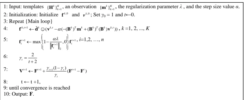
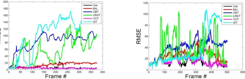
7.1.3. Quantitative evaluations

frame number and the y-coordinate is the RMSE in each frame. Table 3 lists the mean of the RMSEs for all the frames in each of the five sequences. It is seen that the performance of our algorithm is comparable with that of the visual decomposition tracker and that it outperforms the other four algorithms.

Fig. 12. The RMSE curves of the six algorithms for sequence 1. Fig. 13. The RMSE curves of the six algorithms for sequence 2.

Fig. 14. The RMSE curves of the six algorithms for sequence 3. Fig. 15. The RMSE curves of the six algorithms for sequence 4.

Fig. 16. The RMSE curves of the six algorithms for sequence 5.

Table 3: The mean of the RMSEs for all the frames in each of the five sequences

Trackers

Sequences MIL-based

Online Adaboost

L1 regularized

Visual decomposition

Incremental subspace Our

Video 1 13.7 82.7 59.4 4.3 100.7 5.8

Video 2 24.9 40.3 34.3 14.3 40.8 13.9

Video 3 7.8 59.8 106.1 4.2 7.6 4.6

Video 4 27 26.6 27.1 61.6 73.2 8.3

Video 5 32.9 62.7 36.1 129.5 117.5 19.5