Bayesian nonparametric models for spatially indexed data of mixed type

BIROn - Birkbeck Institutional Research Online

Papageorgiou, Georgios and Richardson, S. and Best, N. (2014) Bayesian

nonparametric models for spatially indexed data of mixed type. Journal of

the Royal Statistical Society - Series B (Statistical Methodology) 77 (5), pp.

973-999. ISSN 1369-7412.

Downloaded from:

Usage Guidelines:

Please refer to usage guidelines at or alternatively

Bayesian nonparametric models for spatially indexed data of

mixed type

Georgios Papageorgiou

Department of Economics, Mathematics and Statistics

Birkbeck, University of London, UK

Sylvia Richardson

MRC Biostatistics Unit, University of Cambridge, Cambridge, UK

Nicky Best

Department of Epidemiology and Biostatistics, Imperial College London, UK

Address for correspondence

: Georgios Papageorgiou, Department of Economics,

Mathematics and Statistics, Birkbeck, University of London, Malet Street,

London WC1E 7HX, UK

E-mail: [email protected]

Abstract

We develop Bayesian nonparametric models for spatially indexed data of mixed type. Our work is motivated by challenges that occur in environmental epidemiology, where the usual presence of several confounding variables that exhibit complex interactions and high correlations makes it difficult to estimate and under-stand the effects of risk factors on health outcomes of interest. The modeling approach we adopt assumes that responses and confounding variables are manifestations of continuous latent variables, and uses mul-tivariate Gaussians to jointly model these. Responses and confounding variables are not treated equally as relevant parameters of the distributions of the responses only are modeled in terms of explanatory variables or risk factors. Spatial dependence is introduced by allowing the weights of the nonparametric process priors to be location specific, obtained as probit transformations of Gaussian Markov random fields. Con-founding variables and spatial configuration have a similar role in the model, in that they only influence, along with the responses, the allocation probabilities of the areas into the mixture components, thereby allowing for flexible adjustment of the effects of observed confounders, while allowing for the possibility of residual spatial structure, possibly occurring due to unmeasured or undiscovered spatially varying factors. Aspects of the model are illustrated in simulation studies and an application to a real data set.

1

Introduction

In observational studies the task of identifying important predictors for an outcome of interest can be impeded by the presence of complex interactions and high correlations among confounding variables. Adequately controlling for the effects of such variables can be a challenging task and it may require the inclusion of main and high order interaction effects in the linear predictor of the model, while being subject to multicollinearity problems, which usually lead researchers to select an arbitrary subset of variables to include in the model. Hence, the purpose of this article is to propose a general framework, suitable for spatially structured data, aiming at inferring the effects of explanatory variables on possibly multivariate responses of mixed type, consisting of continuous, count and categorical responses, in the presence of confounding variables, also of mixed type, that can exhibit complex interactions and high correlations.

We consider data observed on the spatial domain, such as point referenced and lattice or regional data. Although in this article we emphasize regional data, as these are predominant in epidemiologic applications which is our specific focus, the presented methods can easily be adapted to accommodate point referenced data. In the sequel, we will use subscript i to denote the ith region, i= 1, . . . , n, of the spatial domain.

Observed data will be classified in three categories. With y_i we will denote a vector of length p of response variables observed in area i. In our context, these will be health outcomes, such as numbers of hospitalizations due to different diseases. Withxiwe will denote a collection of explanatory variables or risk

factors thought to be affecting the response variables. Examples of such variables can include exposure to air pollution and cigarette smoking. Our interest is to directly quantify the effects of explanatory variables on the means of the distributions of the responses. Lastly, with wi we will denote a collection of

confounding variables, i.e. variables that are thought to have an effect on the distribution of the responses but quantification of their effects is not of particular interest. Of interest is only the adjustment for their effects, and that is what distinguishes them from the explanatory variables. Examples of confounding variables can include area-wise ethnic distributions and exposure to socioeconomic deprivation.

Typically, the adjustment for the effects of confounders wi is made by modeling the mean parameter

of the distribution of responses y_i in terms of both confounders wi and explanatory variables xi,using the

usual regression tool. The regression function can also be obtained indirectly, by considering conditional densities of the form f(y_i|xi,wi;θ∗i). Here we propose to adjust for the effects ofwi on the distributions of

the responses y_i by considering joint densities for responses and confounders, f(y_i,wi|xi;θi). Responses

and confounding variables are not treated equally as only parameters describing responses are modeled in terms of explanatory variables.

A benefit of the joint modeling approach is that it frees us from having to include in the linear predictor main and interaction effects of variableswithat are not of particular interest. A difficulty that the proposed

approach creates is that of having to specify densities for the possibly high dimensional vector (y_i,wi).

To mitigate this difficulty and allow for the needed flexibility, we will adopt a Bayesian nonparametric approach. A further criticism is that the approach classifies covariates, (xi,wi), as fixed and random

purely on the basis of the needs of specific data analyses. Hence this classification can change between data analysts depending on their interests, possibly without any theoretical justification as to why this distinction can be made in the first place. See M¨uller et al. (1996) and M¨uller & Quintana (2010) on issues with considering covariates as random.

Our modeling approach is related to that of M¨uller et al. (1996) who jointly modeled continuous data (y_i,xi,wi) using mixtures of multivariate normal densities and adopted a predictive approach in order to

quantify the effects of xi on yi. Although this is a very general approach, in our context quantification

direct quantification of the effects of xi onyi through the regression coefficients.

Other related modeling approaches include those of Shahbaba & Neal (2009) and Hannah et al. (2011). These authors consider joint models for responses and covariates, f(y_i,xi,wi|θ

0

), as in M¨uller et al. (1996), but they further decompose these densities as conditional and marginal densities: f(y_i,xi,wi|θ

0

) =

g(y_i|xi,wi;θ

0

)h(xi,wi|θ

0

). Although this approach performs well in many regression settings, it may continue to be problematic in applications in environmental epidemiology where confounding variables can exhibit interactions and correlations. To see this, consider the case of continuous xi and wi modeled

by a multivariate Gaussian density h(|) with unconstrained covariance matrix. The problems caused by correlated and interacting confounding variables in models of the form f(y_i|xi,wi;θ

∗

i) will also be present

in density g(|) as it expresses the mean of y_i in terms of both explanatory and confounding variables. Here, within a countable mixture framework, we examine two possible remedies for this problem. Firstly, we will consider mixtures of multivariate Gaussians with covariance matrix restricted to be diagonal. A potential effect of this restriction is to decompose the overall dependence among confounding variables into clusters (Henning & Liao, 2013) thereby diminishing the multicollinearity problems within density g(|). Another potential effect of this restriction, however, is to create many small clusters, with a within-cluster regression of y_i on xi providing highly variable posterior samples. Secondly, we will consider densities

g(|) which express the mean of y_i in terms of the explanatory variables only, i.e. densities g(|) with the restriction of regression coefficients corresponding to confounding variables to be equal to zero. Under these constraints, adjustment for the effects of confounding variables is achieved through density h(|).

As indicated earlier, the choice of the priors for θi, i = 1, . . . , n, is crucial in our attempt to flexibly

adjust for confounder effects, while allowing for spatial dependence among observations at nearby areas, potentially occurring due to spatially varying unmeasured or undiscovered factors. Specifically, we adopt a nonparametric approach by which the area specific prior distributions, Pi(θ), are taken to be unknown and

modeled using dependent nonparametric processes. Starting with the early work of MacEachern (1999), dependent nonparametric processes have become increasingly popular due to the flexibility they provide in modeling collections of prior distributions,{P1(.), . . . , Pn(.)},the members of which change smoothly with

covariates, the spatial configuration in our context. Priors Pi(.) corresponding to nearby locations can be

nearly identical while priors corresponding to areas far apart can be quite different. It is this feature of our prior specification that allows for spatial dependence among observations at nearby locations. We induce dependence among the members of the collection of priors by modeling the Pi(.) as countable discrete

mixture distributions with weights indexed byi: Pi(θ) = P ∞

h=1πhiδθh(θ). Here we obtain location-specific

weights by utilizing the probit stick breaking processes of Rodriguez & Dunson (2011) by which the mixture weights are expressed as probit transformations of latent Gaussian Markov random fields (GMRFs) (Rue & Held, 2005). As such, our approach for accounting for potential spatial dependence is related to the approach of Fern`andez & Green (2002) who considered logistic transformations of GMRFs within a finite mixture of Poisson probability mass functions (pmfs) model.

The density of area i takes the form of a convolution fi(yi,wi|xi) =

R

f(y_i,wi|xi;θ)dPi(θ), where,

due to the discreteness of the nonparametric process, density fi can be expressed as fi(yi,wi|xi) =

P∞

h=1πhif(yi,wi|xi;θh), where πhi are location specific weights. The resulting mixture formulation

pro-vides an effective way of estimating the effects of explanatory variables xi on response variables yi, while

adjusting for the effects of confounding variables. To elaborate, adjustment for the effects of confounding variables is achieved by creating clusters of geographical areas that are similar in terms of the observed val-ues of the confounders. With confounding variables having homogeneous valval-ues, a within cluster regression of y onx would reflect the true i.e. unconfounded effects ofx ony in that cluster.

The density of area i can also be expressed as fi(yi,wi|xi) = P ∞

h=1πhig(wi|θh)f(yi|wi,xi;θh) =

P∞

h=1πhi(wi)f(yi|wi,xi;θh), where πhi(wi) = πhig(wi|θh). The last formulation illustrates how both

the proposed model is related to the model for density regression described by Dunson et al. (2007). Conditional models, fi(yi|wi,xi) =

P∞

h=1πhif(yi|wi,xi;θ∗h), in contrast, allow the density to change with

spatial locations only. Furthermore, even with relatively simple, e.g. linear, within cluster regression models, the mixture formulation allows for complex regression functions to be captured. For instance, the joint model fi(yi,wi|xi) as expressed above, implies that E(Yi|wi,xi) =

P∞

h=1πhi(wi)E(Yi|wi,xi;θh).

This method for flexible regression surface estimation was first proposed by M¨uller et al. (1996). The flexibility allowed in the estimation of both the densities and regression surfaces are the reasons for which we opted for mixture based nonparametric methods. There are of course several other approaches to nonparametric Bayesian estimation such as splines, wavelets and neural networks (see M¨uller & Quintana (2004) for a review). However, such methods allow only for flexible estimation of regression surfaces.

With the interpretation given above, the proposed model can be thought of as a spatially varying coefficient model. Alternatives to the proposed model, for univariate responses, build on the work of Besag (1974) and Besag & Kooperberg (1995). Assun¸c˜ao (2003) provided several alternative space varying coefficient models suitable for data observed on small areas. Further, for multivariate small area responses, such models can be constructed utilizing the methods described by Mardia (1988), Jin et al. (2005) and Gelfand & Vounatsou (2003). In this paper, we utilize these methods to construct a spatially varying coefficient model that can accommodate mixed type responses as a means of comparison with the proposed mixture based model.

Our main goal here is to describe general models of the form fi(yi,wi|xi) = P ∞

h=1πhif(yi,wi|xi;θh)

were vectors y_i andwi can include continuous, count and categorical measurements. We jointly model all

measurements by assuming that the discrete ones are discretized versions of continuous latent variables, and using multivariate Gaussians to jointly describe the distributions of observed and latent continuous variables (Muthen, 1984). As such, our approach is related to the recent work of DeYoreo & Kottas (2014) who describe nonparametric mixture models for binary regression, also utilizing latent variables. Models that utilize latent variables, compared to models that assume local independence, allow for more flexible clustering by imposing no unnecessary restrictions on the orientations of the mixture components. Further, in the context of DeYoreo & Kottas (2014), introduction of latent responses is key to flexibly capturing regression relationships.

The remainder of this paper is arranged as follows. Section 2 provides a detailed description of our model formulation. Section 3 provides a brief description of the MCMC algorithm we have implemented, with most of the technical details deferred to the Appendix. Aspects of the model are illustrated in Sections 4 and 5 that present results from simulation studies and an application to a real dataset which examines the association between exposure to air pollution and two birth outcomes. The paper concludes with a brief discussion. Samplers for the described models, and some of their special cases, are available in the R package BNSP (Papageorgiou, 2014).

2

Model specification

The first subsection provides a description of the model formulation for the observed data, while the second one provides a description of how the spatial configuration is build into the model.

2.1

Observed data model

Let y_i = (yi1, . . . , yip)T denote the vector of mixed type responses observed at location i,i= 1, . . . , n. We

assume that the elements of y_i are ordered in the following way: the first p1 of them are counts and they

they are manifestations of continuous latent variables denoted by y∗_i = (y∗_i1, . . . , y_ip∗)T _{(Muthen, 1984). In}

the next few paragraphs we describe the models that connect observed and latent variables.

Firstly, observed counts and corresponding latent variables are connected through the rule: yik =

t1(yik∗, γik) = P ∞

q=0qI[cik,q−1 < y

∗

ik < cik,q], k = 1, . . . , p1. Here, I[.] denotes the indicator function,

cik,−1 = −∞, and for l ≥ 0, cik,l = cl(γik) = Φ−1{F(l;γik)}, where Φ(.) is the cumulative distribution

function (cdf) of a standard normal variable, andF(.;γ) is the cdf of a Poisson(γ) variable. It is clear from the definitions of the cut-points that marginally Yik ∼ Poisson(γik), k = 1, . . . , p1. More generally, one

could take F(.) to be the cdf of a variable that follows some other distribution suitable for modeling count data, such as the negative binomial. Vectors of latent variables underlying counts y(_ia) = (y∗_i1, . . . , y_ip∗₁)T are assumed to independently follow aNp1(0,Σ

(a)

i ) distribution, where Σ

(a)

i is restricted to be a correlation

matrix since the variance parameters are non-identifiable by the data. The present model formulation allows for non-zero correlations among count outcomes (van Ophem, 1999).

Concerning binomial responses, with relevant subscript in the range k = p1 + 1, . . . , p1 +p2, we let

yik =t2(yik∗, πik) =

PNik

q=0qI[cik,q−1 < yik∗ < cik,q], where Nik is the number of binomial trials,cik,−1 =−∞,

and for l ≥1, cik,l =cl(πik) = Φ−1{G(l;Nik, πik)}. Here G(.;N, π) is the cdf of a Binomial(N, π) variable.

Note that, marginally, Yik ∼ Binomial(Nik, πik). Vectors of latent variables y

(b)

i = (y∗i,p1+1, . . . , y

∗ i,p1+p2)

T

are assumed to be independently distributed as Np2(0,Σ

(b)

i ), where Σ

(b)

i , due to identifiability constraints,

is a correlation matrix.

Lastly, for continuous responsesyik,k =p1+p2+1, . . . , p, the corresponding latent variables are directly

observed, yik =yik∗. The distributional assumption about vectors y

(c)

i = (y ∗

i,p1+p2+1, . . . , y

∗

i,p)T, i= 1, . . . , n,

is that they are independent Np3(αi,Σ

(c)

i ) variates.

We let y∗_i = {(y_i(a))T_,(y(b) i )T,(y

(c)

i )T}T denote the vector of latent variables underlying responses at

locationi. It is assumed that the elements ofy∗_i jointly follow a multivariate normal distribution with mean parameter µ(_iy) = (0,0,αi)T, and block covariance matrix Σ

(y)

i with diagonal blocks Σ

(a)

i , Σ

(b)

i , and Σ

(c)

i

defined earlier, and with off diagonal blocks that represent covariances among latent variables underlying different types of responses.

Further, Poisson ratesγik, binomial probabilities πik, and continuous variable means αik are expressed

in terms of risk factors xik, i= 1, . . . , n, k= 1, . . . , p, using canonical link functions (McCullagh & Nelder,

1989): log(γik) = xTikβik, logit(πik) = xikTβik, and αik = xTikβik. In the sequel, we will use symbol xi

to denote all risk factors that correspond to responses observed on area i and symbol β_i to denote the corresponding effects. Further, we will let β ={β_i :i= 1, . . . , n}.

We adjust for the effects of confounding variableswi by including them in the model in a similar way as

the responses, but without modeling parameters of their distributions in terms of risk factors. Confounding variables can also be of mixed type. Specifically we assume that vector wi includes q1 count, q2 binomial,

and q3 continuous variables. Joint modeling is again facilitated by a latent variable representation. Hence,

similar to y∗_i, w∗_i represents the vector of latent variables underlying confounding variables observed at location i, and it is assumed to have a Gaussian distribution with mean µ(_iw) and covariance matrix Σ(_iw). Jointly, y∗_i and w∗_i are assumed to follow a Gaussian distribution with mean µ∗_i = (µ(_iy),µ(_iw)) and covariance matrix Σ∗_i that has diagonal blocks Σ_i(y) and Σ(_iw), while its off diagonal block represents covariances among the two sets of latent variables, cov(y∗_i,w∗_i). We denote µ(w) = {µ(_iw), i = 1, . . . , n}

and Σ∗ = {Σ∗_i, i = 1, . . . , n,}. Further, Poisson rates γ_i(w) = (γ_i(₁w), . . . , γ_iq(w₁))T and binomial probabilities

π_i(w)= (π_i(₁w), . . . , π(_iqw) 2 )

T _{of confounding variables will collectively be denoted by γ}(w) _{and π}(w)_.

Withθi = (βi,Σ ∗ i,µ

(w)

i ,γ

(w)

i ,π

(w)

the form

f(y_i,wi|xi;θi) =

Z

. . .

Z

N(y∗_i,w∗_i|µ∗_i,Σ∗_i)dy∗_idw∗_i,

where the integral is with respect to latent variables underlying Poisson and binomial counts of response and confounding variables, with integral limits that depend on (β,γ(w)_,π(w)_).

For all areas it is assumed that (y_i,wi) arises from a convolution density of the form

fi(yi,wi|xi) =

Z

f(y_i,wi|xi;θ)dPi(θ), (1)

where Pi(.) are location specific mixing distributions that are regarded as unknown and thus assigned a

probit stick breaking process prior (Rodriguez & Dunson, 2011). Hence, they are represented as

Pi(.) = ∞

X

h=1

πhiδ_θ

h(.), (2)

where the atoms θh = (βh,Σ ∗ h,µ

(w)

h ,γ

(w)

h ,π

(w)

h ) are assumed to independently arise from the base

dis-tribution G0 which consists of independent priors. More details on these priors are provided in Section

3.

2.2

Probit stick-breaking process priors

Spatial dependence among measurements at nearby locations is induced by constructing the weights of the stick-breaking processes as probit transformations of latent variables that arise from Gaussian Markov random fields (Rue & Held, 2005). These random fields are multivariate normal distributions defined on an undirected graph with areas represented by nodes and neighboring areas connected by an edge. Here areas are taken to be neighbors if they are geographically contiguous.

Mixture weights are obtained as

πhi= Φ(ηhi)

Y

l<h

{1−Φ(ηli)},

where ηhi = α+uhi/φ, and the Gaussian Markov field realizations uh = (uh1, . . . , uhn)T are obtained as

independent draws from Nn(0,Q−_λ1), h ≥ 1. The precision matrix is given by Qλ =λA+In, where the

adjacency matrix A = {aii0}n

i,i0₌₁ is defined as follows: a_ii = ν_i, the number of neighbors of area i, and

for i6=i0, aii0 =−1 if locations i and i0 are neighbors, and a_ii0 = 0 otherwise (Fern`andez & Green, 2002).

Thus, the probability density function (pdf) of uh,h≥1, can be expressed as

p(uh|λ) = c(λ) exp

−1

2u

T hQλuh

= c(λ) exp

"

−1

2

(

λX

i0_∼i

{uhi−uhi0}2+

n

X

i=1

u2_hi

)#

, (3)

where P

i0_∼i denotes the sum over all pairs of neighbors. The normalizing constant c(λ) is given by

c(λ) = (2π)−n/2Qn

i=1(λei+ 1)

1/2_{, where e}

1, . . . , en, denote the eigenvalues of the adjacency matrixA.

The non-negative parameterλdetermines the spatial correlation among the elements ofuh, with higher

the elements of uh. The magnitude of λalso determines the amount of shrinkage of the adjacency matrix

A towards the identity matrix, In. The effect of this shrinkage is to ensure that precision matrix Qλ is

positive definite.

This model formulation allows for the possibility that observations that correspond to nearby areas are more likely to have similar values for the component weights than observations from areas that are far apart. Although parameter λ clearly determines the correlations among the elements of the GMRFs, correlations among component weights depend on the combinations of values of the parameters that govern the GMRFs: (α, φ, λ). For instance a high value of λ combined with a high value of φ implies smaller correlations among the component weights than the correlations implied by a high value of λ combined with a small value of φ.

3

Prior specification and MCMC sampler

We develop a sampler that uses ideas from the work of Rodriguez & Dunson (2011) and implements the label switching moves suggested by Papaspiliopoulos & Roberts (2008). We focus on the case where there is one response of each type and q continuous confounders. Samplers for more general models can be constructed as a direct generalization of the presented sampler.

With y_i = (yi1, yi2, yi3)T denoting the vector of count, binomial and continuous responses, y∗i =

(y_i∗₁, y∗_i2, y∗_i3)T _{denoting the corresponding latent variables, and w}

i = (wi1, . . . , wiq)T denoting the vector of

confounders observed on location i, i= 1, . . . , n, the model is formulated as

vi ≡((y∗i) T

,wT_i )T|{µ∗_i,Σ∗_i} ∼Ns µ∗i =

αi

µ(_iw)

, Σ∗_i =

"

Σ(_iy) Ci

CT_i Σ(_iw)

# !

, (4)

where s= 3 +q, E(y∗_i) =αi, E(wi) = µ

(w)

i , var(y ∗ i) =Σ

(y)

i , var(wi) =Σ

(w)

i , and cov(y ∗

i,wi) = Ci. Recall

that the first two elements of αi are constrained to be zero and the third one is modeled as αi3 =xTi3βi3.

Hence, the meanµ∗_i can be expressed asµ∗_i =X∗_iξ_i, whereξ_i = (β_iT₃,(µ_i(w))T₎T_{, andX}∗

i is a design matrix

the first two rows of which include only zeros in order to satisfy the requirement of zero means: E(y_i∗₁) = 0, E(y_i∗₂) = 0. Further, the first two diagonal elements of Σ∗_i are constrained to be one. Lastly, Poisson rates

γi and Binomial probabilitiesπi are modeled as: log(γi) = xTi1βi1 and logit(πi) =xTi2βi2, i= 1, . . . , n.

The joint density of the data observed on the ith location (y_i,wi) takes the form

f(y_i,wi|xi;θi) =

Z Ωi2

Z Ωi1

Ns(vi|µ∗i,Σ ∗ i)dy

∗ i1dy

∗

i2, (5)

where Ωi1 = (ci,1,yi1−1, ci,1,yi1), Ωi2 = (ci,2,yi2−1, ci,2,yi2), andθ = (βi1,βi2,ξi,Σ ∗

i) denotes model parameters.

3.1

Posterior sampling

First note that from (1), or its special case (5), and (2), the density of (y_i,wi) can be expressed as a

countable mixture of densities, which we approximate by a truncated mixture

fi(yi,wi|xi) = T

X

h=1

πhif(yi,wi|xi;θh). (6)

Introducing the usual allocation variablesδi, model (6) can equivalently be written as

y_i,wi|θ, δi =ki ∼f(yi,wi|xi;θki),

Further augmenting with latent variables underlying discrete responses y∗_i,1:2 = (y_i∗₁, y_i∗₂)T_{, we obtain the}

‘complete data’ likelihood

`({y_i,wi, δi =ki,y∗i,1:2 :i= 1, . . . , n}) =

n

Y

i=1

I[y_i∗₁ ∈Ωi1]I[yi∗2 ∈Ωi2]Ns(vi|ξki,Σ ∗

ki)πkii ,

and the sampler updates from π(θ,δ,η, α, φ, λ,y∗|y,w)∝g1(y|y∗,δ,θ)g2(y∗,w|δ,θ)

g3(δ|η)g0(θ,η, α, φ, λ)∝

n

Y

i=1 n

I[cyi1−1(Eiγki)< y

∗

i1 < cyi(Eiγki)]

I[cyi2−1(πki)< y

∗

i2 < cyi(πki)]Ns(vi|ξki,Σ ∗ ki)πkii

o

g0(θ,η, α, φ, λ),

whereEidenotes the expected number of counts in areai. Further details on the MCMC steps are provided

in the Appendix.

Prior specification g0(θ,η, α, φ, λ) utilizes independent priors for parameters βh1, βh2, ξh, and Σ ∗ h,

h ≥ 1. We describe these in the following subsection. Priors for other parameters can be found in the Appendix.

3.2

Specification of the base distribution and hyperparameters

First, the priors for effects of the risk factors on the Poisson rates and binomial probabilities are specified as: β_hk ∼Nrk(βhk;0, τ2I), whererk denotes the dimension,k = 1,2. Similarly, the prior on ξh is taken to

be ξ_h ∼Nr3+q(ξh;µξ,Dξ), where µξ = (0T,w¯T)T. Here ¯w denotes the empirical mean of the confounding

variables and Dξ is a diagonal matrix of τ2 (repeated r3 times) followed by the empirical variances of the

confounding variables. In our analyses we take τ2 = 25.

We specify prior distributions on the restricted covariance matrices Σ∗_h, h≥ 1, by incorporating addi-tional variance parameters into the model that are non identifiable by the data (Zhang et al., 2006) and separating identifiable from non identifiable parameters using the separation strategy of Barnard et al. (2000). Specifically, we start by specifying Wisharts(Eh;η,H) priors for unrestricted s× s covariance

matrices Eh, h≥1:

p(Eh|η,H)∝ |Eh|(η−s−1)/2etr(−H−1Eh/2), (7)

where etr(.) = exp(tr(.)), and

H =

H11 H12

HT₁₂ H22

,

where H11 is a 3×3 covariance matrix with its first two diagonal elements restricted to be one, H22 is a

q×q unrestricted covariance matrix, and H12 is a 3×q matrix of covariances.

We decomposeEh =D

1/2

h Σ

∗ hD

1/2

h into a diagonal matrix of two (non identifiable) variance parameters

and 1 + q ones (corresponding to identifiable variances), that is, Dh = Diag(d2h1, d 2

h2,1, . . . ,1), and a

covariance matrixΣ∗_h that has the required form. The Jacobian that is associated with this transformation is J(Eh →Dh,Σ∗h) =

Q2

j=1d (s−1)

hj =|Dh|

(s−1)/2_{, and along with (7) it implies a joint pdf for (D}

h,Σ∗h):

p(Dh,Σ∗h|η,H)∝ |Eh|(η−s−1)/2etr(−H−1Eh/2)J(Eh →Dh,Σ∗h). (8)

We take (8) to be the joint prior for (Dh,Σ∗h). Concerning posterior sampling, we will sample these two

4

Simulation studies

4.1

First simulation study

There are two main goals in the first of the two simulation studies that we present here. The first goal is to compare the proposed model with the related models that were briefly described in the introductory section of the paper. These models will be described in more detail in the next few paragraphs. The second one is to appraise two of the aspects of the proposed model, namely the inclusion of the spatial structure and the continuous latent variable representation of the discrete variables, by comparing the model with special cases of it that do not take the spatial configuration into account and/or assume that discrete variables are conditionally independent.

Both simulation studies are carried out on the spatial layout of then= 94 mainland French d´epartments. In the first scenario that we present here a count response is assumed to be influenced by one continuous confounding variable and one continuous risk factor. Univariate responses, risk factors and confounders will be denoted by yi, xi,and wi,while expected counts will be denoted byEi. The latter will be obtained

as Ei iid

∼Uniform(10,20).

Given the above data specifications, the proposed model, which in the sequel we will denote by M1,

takes the form: fi(yi, wi|xi) =PT_h=1πhif(yi, wi|xi;θh). Details on M1 were provided in Section 3. Here we

note that the within component Poisson relative risks are expressed asγih= exp(β0h+β1hxi). We compare

M1 with the model proposed by Shahbaba & Neal (2009) and Hannah et al. (2011), denoted by M2 and

expressed as: fi(yi, wi|xi) = P_hT₌₁πhig(yi|xi, wi;θ0h)k(xi, wi|θ0h). Here g(yi|xi, wi;θ0h) denotes a Poisson

pmf with relative risk γih= exp(β0h+β1hxi+β2hwi), whilek(xi, wi|θ0h) denotes a bivariate Gaussian with

unconstrained covariance matrix.

We further consider two variations of M2. The first one, which we will denote by M3, imposes a diagonal

covariance matrix in the multivariate Gaussian k(|). The second one, denoted by M4, imposes regression

coefficients corresponding to confounding variables in the Poisson model g(|) to take value zero. That is, M4 sets β2h = 0 for all h. As explained in the introduction, with these two constraints we attempt to

mitigate the problems caused by high correlations and/or complex interactions, firstly by decomposing the overall dependence into clusters (M3) and secondly by removing confounding variables from the Poisson

model and adjusting for their effects through the multivariate Gaussian (M4).

In addition, we consider a similar model to the one proposed by Fern`andez & Green (2002) and Green & Richardson (2002), which takes the form fi(yi|xi, wi) =

PT

h=1πhif(yi|xi, wi;θ∗h). This model

is a countable mixture of Poissons, where the component specific relative risks are expressed as γih =

exp(β0h+β1hxi+β2hwi). We will denote this model by M5.

Lastly, we consider two spatially varying coefficient models. At the observed level, both models are expressed as:

Yi ∼ Poisson(Eiλi),

log(λi) = β0i+β1iXi+β2iWi, i= 1, . . . , n.

Let βki =βk+bki, k= 0,1,2, and bi = (b0i, b1i, b2i)T, i= 1, . . . , n. In the first specification, bi are modeled

using an improper multivariate conditionally autoregressive (CAR) distribution:

bi|{bj, j 6=i},Ω−1 ∼N3(n−i 1

X

j∼i

bj, n−i 1Ω −1_).

Model M1 takes the spatial configuration into account and it also allows for non-zero within cluster

correlation between continuous confounding and discrete response variables. We assess these two features of the model by comparing its performance with the performances of three models that are special cases of it, namely:

M1A: a model that ignores possible spatial dependence by placing a degenerate at zero prior distribution

on parameter λ, but that allows for non-zero within cluster correlation between confounding and response variables,

M1B: a model that takes into account possible spatial dependence, but that assumes within cluster

inde-pendence among confounding and response variables, that is, a model that describes component h

using the product density f(yi, wi|xi;θh) = Poisson(yi|xi;γh)N(wi|µh, σh2), and

M1C: a model that ignores possible spatial dependence and that assumes within cluster independence

among confounding and response variables.

We compare the models on the basis of their ability to recover the spatially varying risk factor effects. For this comparison we utilize the posterior mean squared error (MSE) that quantifies the discrepancy between true β1i and estimated ˆβ1i risk factor effects: MSE(β1i) =E{(β1i−βˆ1i)2|data}, i= 1, . . . , n. As a

one number summary that captures the performance of the models over the whole map, we calculate the root averaged mean squared error: RAMSE(β₁) = (P

iMSE(β1i)/n)

1/2_{. Similarly, we calculate summaries}

over selected clusters of geographical areas.

In the current simulation study, then = 94 French departments were divided into four clusters. These are shown in Figure 1 (a) along with the true model parameters. Thirty datasets (N=30) were generated by the following two stage process. At the first stage, continuous latent variables and risk factors, y_i∗, x∗_i, and directly observed confounding variables, wi, were obtained as realizations from a trivariate normal

distribution. For instance, for the north-east (NE) cluster of areas, these were obtained from

(y_i∗, x∗_i, wi)T

iid

∼N3  

 

0.0 0.0 10.0

 ,

 

1.0 0.0 0.0 0.0 1.0 0.0 0.0 0.0 1.0

 

 .

Parameters of the other three Gaussians are shown in Figure 1 (a). Note that, for all clusters we set E(y∗_i) = 0.0, E(x∗_i) = 0.0, var(y∗_i) = 1.0, var(x_i∗) = 1.0, and cor(y_i∗, x∗_i) = ρy∗_ix∗_i = 0.0, and hence these are

not shown on Figure 1 (a). Figure 1 (b) shows pairs (wi, yi∗), i = 1, . . . ,94, from one of the 30 realized

datasets, along with 95% ellipsoids for the respective bivariate Gaussians.

At the second stage, risk factors, xi, were obtained from x∗i as: xi = 3Φ(xi∗)−3E{Φ(x∗i)}, so that

xi ∼ Uniform(−1.5,1.5). This two stage process allows the correlations cor(y∗i, xi) and cor(xi, wi) to be

close to the desired ones, cor(y_i∗, x∗_i) and cor(x∗_i, wi), respectively. Furthermore, latent variables underlying

counts were discretized using cut-points that respect the desired relative risks and risk factor effects. Specifically, Poisson counts were obtained as yi = q, where q satisfies: Φ−1{F(q−1;Eiexp(β0 +β1xi +

β2x2i +β3wi))}< y∗i <Φ

−1_{F(q;E

iexp(β0+β1xi+β2x2i +β3wi))}. Here Φ(.) and F(.;.) denote the cdfs

of the standard normal and Poisson distributions.

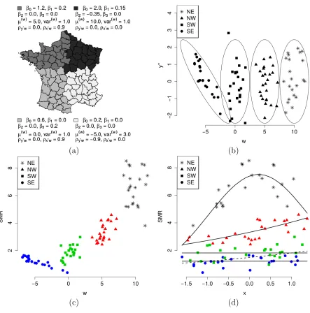
(a) (b)

(c) (d)

Figure 1: First simulation study cluster structure and data. (a) Map of mainland French departments divided into four clusters and true cluster parameters. Parameters µ(w) and var(w) are the mean and variance of the confounding variables. Parameter ρy∗_w denotes the correlation between latent variables

underlying counts and confounding variables, while parameter ρx∗_w denotes the correlation between the

variable, yi. Similar is the within SW cluster challenge: there is high correlation between xi and wi, but

only wi has an effect on yi. Lastly, within the SE cluster, the response variable is only related to the

confounding variable, not through the regression coefficient β3, but through the high negative correlation

between wi and yi∗. To stress this relationship in the SE cluster, we have chosen the variance of wi to be

higher than the corresponding variances within the other three clusters.

For one of the N = 30 generated datasets, Figure 1 (c) presents a scatter plot of realized confounding variables against observed area relative risks. The latter are also known as standardized mortality ratios (SMRs), obtained as: SMRi =Yi/Ei. It is evident that there is enough separation among the four clusters

in terms of wi. Hence, models that cluster areas according towi, that is models M1 - M4, are expected to

have an advantage over models that do not, that is models M5 and M6. We see that within the NE cluster,

yi and wi are unrelated. Within the NW cluster, they are positively related. This is a result of the positive

relationship between yi and xi and the positive relationship between xi and wi. Within the SW cluster,

the positive relationship between yi and wi is a result of the positive regression coefficient,β3 = 0.2, while

the negative relationship within the SE cluster is a result of the negative correlation between y∗_i and wi.

Similarly, Figure 1 (d) is a scatter plot of the explanatory variable against the SMRs. The Figure shows the quadratic relationship within the NE cluster, the linear relationship within the NW cluster, and the lack of relationship within the SE cluster. Within the SW cluster, xi andyi are unrelated (indicated by the

solid line) but the realized dataset shows a positive relationship due to the positive relationship between

yi and wi and the positive relationship betweenwi and xi (indicated by the dashed line).

Results are obtained based on 50,000 posterior samples, after a burn in period of 10,000 samples, for each of the N = 30 datasets, and are displayed in Figures 2 and 3, and Table 1. We first examine Figure 2 and Table 1 that present summaries concerning the estimation of the spatially varying regression coefficients, and focus on comparing the performances of models M1-M6. Figure 2 displays the within

cluster curves that were obtained at every 50th iteration of the samplers of models M1 and M2, for one

particular simulated dataset, along with the true curves. Note that, curves from model M3 and M4 are

indistinguishable from those of models M2 and M1 respectively, and hence not displayed. Further, model

M5does not identify the clustering correctly and thus results from it are not displayed either. It can be seen

from Figure 2 that the quadratic relationship between explanatory variable and log SMR within the NE cluster is captured by splitting the cluster into 2 sub-clusters: in one there is a positive linear relationship and in the other one a negative linear relationship. Within the NW cluster, that is characterized by a linear association between risk factor and log relative risk, and by high correlation between confounder and risk factor, models M1 and M4 that do not include the confounding variable in their linear predictors identify

the true relationship with higher certainty than models M2 and M3. This is evident from both Figure

2 and the first row of Table 1. From the latter we see that M1 and M4 have the smallest RAMSE(β1),

while M3 and M5 have the highest, and M2 and M6A have middle range RAMSEs. The RAMSE of M6

is several times larger in every cluster than the RAMSE of every other model as it cannot cope with the high correlations between xand wthat are present in some of the clusters. For this reason we exclude this model from further comparisons. Continuing with the SW cluster in which there is a linear relationship between confounding variable and log relative risk, and high correlation between confounding variable and risk factor, models M1 and M4 overestimate the regression coefficient β1, that is they cannot distinguish

the causal effect from the effect that is due to the high correlation (Figure 2). Models M2 and M3, that

include the confounding variable in their linear predictors, provide, due to multicollinearity, highly variable estimates of β1 with posterior credible intervals that include the true value of the parameter. In terms of

RAMSE(β₁), M6A has the lowest while M3 the highest. Lastly, within the SE cluster, in which there is no

direct or indirect relationship between risk factor and risk, models M1, M2 and M6A do reasonably well in

estimating β1 (Figure 2), with M1 having the smallest RAMSE and M5 the highest (Table 1).

M1 M2

Figure 2: First simulation study results: within cluster model fits obtained at every 50th iteration of the samplers of models M1 and M2 for one of the thirty simulated datasets along with the true curves.

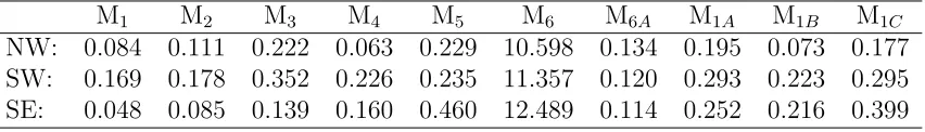
Table 1: First simulation study results: average RAMSE(β₁) (over the N = 30 simulated datasets) over the three geographical clusters where the relationship between log SMR and risk factor is linear.

M1 M2 M3 M4 M5 M6 M6A M1A M1B M1C

NW: 0.084 0.111 0.222 0.063 0.229 10.598 0.134 0.195 0.073 0.177 SW: 0.169 0.178 0.352 0.226 0.235 11.357 0.120 0.293 0.223 0.295 SE: 0.048 0.085 0.139 0.160 0.460 12.489 0.114 0.252 0.216 0.399

1 that M1A that ignores spatial configuration does worse than M1 in all geographical clusters. The obvious

value of taking the geographical configuration into account in capturing the spatially varying coefficients is also illustrated by comparing models M1B and M1C. Comparing now model M1B, that assumes within

cluster independence, with M1, we see that M1B does better in the NW cluster where the assumption of

local independence holds (ρy∗_w =β₃ = 0). However, M_1B does worse than M₁ in the SW and SE clusters,

where the assumption of local independence does not hold. Comparison of the RAMSEs from models M1A

and M1C further illustrates the points related to local independence.

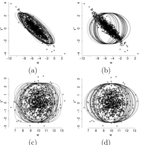
Lastly, Figure 3 shows the extra clustering flexibility gained by avoiding the assumption of local in-dependence. Figures 3 (a) and (b) show realized pairs of (w, y∗) from the bivariate normal density that describes the SE cluster of areas. Ignoring the location parameters, the bivariate normal has parameters var(y∗) = 1.0, var(w) = 3.0, and cor(y∗, w) = −0.9. Figure 3 (a) shows how model M1 deals with this

negative dependence. The Figure displays, along with realized pairs, 95% ellipsoids that were obtained in the simulation study from model M1. Ignoring the dependence parameter, i.e. setting cor(y∗, w) = 0.0, as

in M1B, results in a considerably worse fit, as illustrated in Figure 3 (b).

(a) (b)

(c) (d)

Figure 3: First simulation study results: scatter plots of (w, y∗) pairs obtained from the bivariate Gaussians that describe the SE, (a) and (b), and NE, (c) and (d), clusters along with 95% ellipsoids obtained from models M1, (a) and (c), and M1B, (b) and (d).

4.2

Second simulation study

The purpose of the second simulation study is to evaluate the non-parametric structure when the true data generating mechanism is a generalized linear mixed effects model with random intercepts obtained as realizations form a GMRF, but with no further covariates or confounders.

More comprehensive comparisons between CAR type models and mixtures of Poisson pmfs can be found in Fern`andez & Green (2002), Green & Richardson (2002) and Best et al. (2005). These have concluded that 1.even when the true underling model is a CAR type model, mixture models perform very competitively, and 2. when there are discontinuities in the risk surface, mixture models outperform CAR models as the latter lack a mechanism for dealing with gaps and hence they oversmooth the risk surface. Below we describe in more detail our simulation study.

The synthetic datasets are obtained by a two stage process. At the first stage a GMRF u is obtained from the proper pdf p(u|λ) given in (3). At the second stage, count responses are generated as Yi ∼

Poisson(Eiexp(ηi)), where ηi =ui/φ, Ei iid

∼ Uniform(10,20), i = 1, . . . , n. We have selected four different values for λ and 1/φ, which are shown in Table 2. For each combination of the two parameters, we generated N = 20 datasets and fitted nonparametric and CAR models.

The nonparametric model takes the form fi(yi) =

P

hπhig(yi|θh), where g(.|θ) denotes a Poisson pmf

with relative risk θ. This model is a special case of M5 that has no covariates and it is reminiscent of the

model proposed by Fern`andez & Green (2002). The CAR model is expressed as Yi ∼Poisson(Eiexp(θi)),

where θi ∼N(n−i1

P

j∼iθj, n−i 1τ2), i= 1, . . . , n, reminiscent of the model by Besag et al. (1991).

We summarized the performances of the two models calculating the RAMSE= ((N n)−1PN

k=1 Pn

i=1(ηi−

ˆ

ηi)2)1/2.

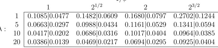
Table 2: Second simulation study results: the first (second) entry in each cell is the RAMSE obtained from the nonparametric (CAR) model.

1/φ

1 21/2 2 23/2 1 0.1085|0.0477 0.1482|0.0609 0.1680|0.0797 0.2702|0.1244

λ: 5 0.0663|0.0297 0.0988|0.0434 0.1161|0.0529 0.1341|0.0594 10 0.0417|0.0202 0.0686|0.0316 0.1017|0.0404 0.0964|0.0385 20 0.0386|0.0139 0.0469|0.0217 0.0694|0.0295 0.0925|0.0404

times larger than those obtained from the CAR model, with small variation around this number. Lastly, it is interesting to observe that RAMSEs increase with increasing variance 1/φ and decrease with increasing spatial association parameter λ.

5

An examination of the association between birth outcomes

and exposure to ambient air pollution

We apply the proposed model to study the association between two birth outcomes and exposure to ambient air pollution. The birth outcomes that we consider are preterm birth and birth weight. Both of these serve as proxy measures of the degree of biological maturity of the fetus for supporting extrauterine life. As a measure of air pollution we consider the total suspended particulate matter (PM) equal to or less than 10 micrometers (µm) in diameter (PM10).

Preterm birth is defined as delivery before 37 completed weeks of gestation (birth occurring at least four weeks before the estimated date of delivery). Determining, however, when natural conception takes place, and hence gestational age at birth, has been difficult. For this reason, birth weight was originally used as a proxy measure for maturity. The main issue, however, with birth weight as a proxy of immaturity is that it may misclassify many infants, for instance those who have small/large weight for their gestational age. Hence, gestational age is considered as a better surrogate of maturity and it is preferred over birth weight, whenever it is available (see e.g. Behrman & Butler (2007)). Here, the response variables that we consider are the dichotomous Y1 : gestational age at birth ≤37 weeks, and the continuous Y2 : birth weight.

Several epidemiological studies have examined the relationship between environmental air pollution exposures and preterm birth and birth weight, with, however, unclear results. For instance, a recent systematic review and meta-analysis (Stieb et al., 2012) reports that the majority of the studies reviewed, found that increased air pollution was associated with reduced birth weight. However, the authors also reported evidence of publication bias. Further, the same authors reported that the estimated effects on preterm birth were mixed. Inconsistent results have also been reported elsewhere, see e.g. Behrman & Butler (2007) and references therein. The majority of these studies considered birth weight as the response variable due to the difficulties with gestational age mentioned above. For instance in Stieb et al. (2012) there are 62 (8) studies that consider weight (gestational age) as the response. Here, we add to the literature a study that considers both responses simultaneously, and can thus shed light on how the air pollution effects on the two responses compare.

the model area level lung cancer occurrence counts. This is the first confounding variable that we include in the model, denoted by W1, and it serves as proxy to smoking rates (Best & Hansell, 2009).

In addition, several studies have documented significant associations between area-level characteristics and birth outcomes, see e.g. Elo et al. (2001) and Behrman & Butler (2007, pages 137-147) and references therein. Area-level characteristics such as crime rates and socioeconomic deprivation can influence health outcomes through pathways such as exposure to acute or chronic stress and availability of social support and goods and services. We account for area level characteristic by including in the model (sub)-domains of the Index of Multiple Deprivation 2010 (IMD) (Department for Communities and Local Government, 2011). Specifically, we include the domains of ‘Income’ deprivation, ‘Crime rates’, ‘Distance to local services’ (services such as general practice surgery and stores) and ‘Housing quality’. For all domains higher scores indicate relatively less advantaged areas. However, only ‘Income’ deprivation scores are expressed in meaningful units. These represent proportions of income deprived people in the areas. The construction of all other domain scores, including the overall IMD score, involves an exponential transformation that results in deprivation scores that are difficult to interpret. We overcome this difficulty by ranking the domain scores and dividing the ranks by the total number of areas. These new scores are more meaningful: the score of a given area represents the proportion of areas that are less deprived than that area.

Furthermore, there is evidence of significant differences in birth outcomes among different ethnic groups (Behrman & Butler, 2007). Hence, we adjust our analysis for area-wise ethnic distributions, expressed as percentages of people whose ethnic background can be described as White, Asian, or Other, denoted by

pw, pa, and po. We include two of these percentages in the model after applying a ‘logit’ transformation:

p∗_a = log{pa/pw}, p∗o = log{po/pw}. The purpose of these transformations is to create variables that have

the real line as their support so that they can be modeled by a mixture of multivariate normal densities. Lastly, as it is well known that maternal age can have important effects on birth outcomes (see e.g. (Behrman & Butler, 2007, pages 44-47)) we adjust our analysis for the area-wise mean maternal age.

By utilizing the proposed model we can examine the effect of ambient air pollution on the two birth outcomes of interest while automatically adjusting via the clustering aspect of the model for the possibly nonlinear effects of the other risk factors and their interactions. The latter can be important in this application as nonlinear and interaction effects among the aforementioned risk factors have been described in the literature. For instance, Alexander et al. (1999) found that racial/ethnic differences in birth weights become more pronounced as pregnancies approach term. In addition, nonlinear effects of maternal age on the risk of preterm birth have been described Behrman & Butler (2007, pages 125-127): there is higher risk associated with young maternal ages and ages over 35. Furthermore, the effect of maternal age on preterm birth varies among racial/ethnic groups. For instance, the risk of preterm birth starts to increase at a later age for whites than for blacks, and this increase is slower for whites.

We examine whether maternal exposure to PM10 increases the risk of adverse birth outcomes in a

small area study involving the n = 628 Output Areas (OA) of Greater London, 2008. The two response variables that we consider are Yi1 the number of preterm births in areai, and Yi2 the average birth weight

in area i. Note that, as multiple gestations is one of the strongest risk factors for premature birth, we confine our analysis to singleton births. Given the total number of singleton births per area, Ni, variable

Yi1 is modeled asYi1 ∼Binomial(πi, Ni), where logit(πi) = xTi1βi1 =βi,01+βi,11PM10,i, where P M10,i is the

estimated annual average exposure to PM10 in area i. Variable Yi2 is modeled as Yi2 ∼N(αi, σi22), where

αi =xTi2βi2 =βi,02+βi,12PM10,i+βi,22Oi, with Oi =Yi1/Ni denoting the observed proportion of preterm

births in area i. Hence, the model for the latent and observed continuous response variables (y_i∗₁, yi2) for

area itakes the form

(y_i∗₁, yi2)T|{βi,Σ ∗

i} ∼N2

βi,01+βi,11PM10,i

βi,02+βi,12PM10,i+βi,22Oi

,

1.0 σ12

σ21 σ22

Figure 4: Estimated average annual exposure to PM10.

The inclusion of the proportion of preterm births Oi as a covariate for birth weight Yi2 defines a

recur-sive model. Such models are extenrecur-sively used in the econometric literature to adjusted for unobserved confounding, see e.g. Heckman (1978) and Goldman et al. (2001) for an application in biostatistics.

The number of lung cancer occurrences, the first confounding variable Wi1, and age-sex distribution

for each OA were available in 5-year age bands. The expected number of lung cancer occurrences, Ei, i=

1, . . . , n, were calculated based on the age-sex distributions, thereby adjusting for these two important risk factors. Counts where modeled as Wi1 ∼ Poisson(Eiγi), where γi = exp(βi,03). Additional confounders

included in the model are the four IMD (sub)-domains, Wi2, . . . , Wi5, two variables describing the ethnic

distribution, Wi6 and Wi7, and maternal age Wi8.

The model we fit takes the form fi(yi,wi|xi) =

P∞

h=1πhif(yi,wi|xi;θh). It is a joint model of two

discrete variables, the Binomial Yi1 and count Wi1, and eight continuous ones, Yi2 and Wi2, . . . , Wi8.

Only the means of the response variables, Yi1, Yi2, are modeled in terms of explanatory variables, xi1 =

(1,PM10,i)T andxi2 = (1,PM10,i,Oi)T respectively. Further, variablesWij, j = 1, . . . ,8,are jointly modeled

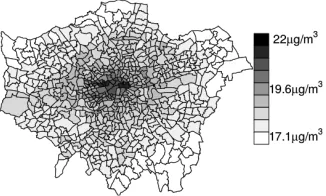
with the responses in order to adjust for their effects. Data and results are displayed in Figures 4 - 7. First, Figure 4 displays the estimated average annual exposures to PM10. These range from 17.1 to 22

µg/m3_{, with average exposure equal to 18.6 µg/m}3_{, and interquartile range of 1 µg/m}3_.

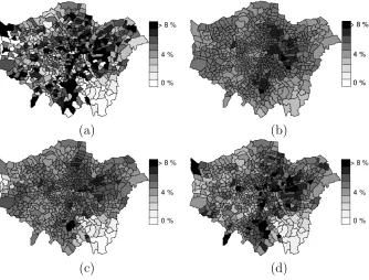
Figure 5 (a) displays the observed area-wise probabilities of preterm birth. Smooth estimates recovered from the proposed model are displayed in Figure 5 (b). They are obtained as follows: for each area

i, i = 1. . . , n,and for each iteration of the sampler t, t= 1, . . . , T, we observe the cluster assignment and the regression coefficients associated with this cluster. Denote these by z_i(t) and β(_i1t) respectively, where

β(_i1t) depends on i through z_i(t). The model based estimate of the probability of preterm birth in area i

at iteration t is obtained as π_i(t) = logit−1(xT i1β

(t)

i1), while the smooth model based estimate of the same

probability is obtained as median(π_i(1), . . . , π_i(T)).

For a comparison, we also obtained smooth model based estimates of the probabilities of preterm birth by generalizing the model proposed by Fern`andez & Green (2002) to handle mixed type outcomes. These are shown in Figure 5 (c). We have also fitted a multivariate generalized linear mixed model with random effects that have multivariate conditionally autoregressive (MCAR) distributions (see e.g. Mardia (1988), Gelfand & Vounatsou (2003), Jin et al. (2005)). These are shown in Figure 5 (d). Briefly, the model of Fern`andez & Green (2002) here is expressed asfi(yi|xi,wi) =P

∞

h=1πhif(yi|xi,wi;θh). It is a joint model

of two response variables, the binomial Yi1 and the continuous Yi2, where the corresponding latent and

observed continuous variables, y_i∗₁ and yi2, are modeled as

y∗_i1 =xT_i1β_i,11+wT_i β_i,21+i1

yi2 =xTi2βi,12+w

T

(a) (b)

(c) (d)

Figure 5: Probabilities of preterm birth: (a) observed, and smoothed utilizing (b) the proposed model, (c) the model of Fern`andez & Green (2002), and (d) an MCAR model.

and the bivariate error term is assumed to be distributed as

1i

2i

iid

∼N2

0 0

,

1 σ12

σ21 σ22

.

Continuing now with the MCAR model, it is expressed as

Yi1 ∼ Binomial(Ni, πi)

logit(πi) = xTi1β11+wTi β21+xTi1βi,11+wTi βi,21

Yi2 = xTi2β12+wTi β22+xTi2βi,12+wTi βi,22+i,

where {β_i,11,β_i,21,β_i,12,β_i,22 : i = 1, . . . , n} denote area-specific random effects. For random effects that appear in only one of the response models, a univariate CAR model is assumed, while for effects that appear in both, a bivariate CAR model is specified. For instance, the observed proportion of preterm births Oi

is included only in the model of birth weight Yi2, and the corresponding random effects β∗ = (β1∗, . . . , βn∗)

are modeled as

β_j∗|β_−j∗ , τ2 ∼N(X

i∼j

β_i∗/nj, τ2/nj),

where nj denotes the number of neighbors of area j, and τ2 is a variance parameter.

All other random effects are independently modeled using bivariate CAR distributions. For instance, random effects corresponding to PM10, βi,11= (βi,111, βi,121)T, i= 1, . . . , n,

β_j,11|β−j,11,V ∼N2( X

i∼j

(a) (b)

(c) (d)

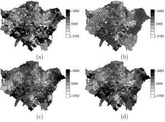
Figure 6: Birth weight: (a) observed, and smoothed utilizing (b) the proposed model, (c) the model of Fern`andez & Green (2002), and (d) an MCAR model.

where V is a 2×2 positive definite matrix.

By comparing Figure 5 (b) to (c) and (d), it appears that the proposed model results in smoother estimates of the preterm birth probabilities. This can be attributed to the fact that the proposed model fits a simple response model within each component. This results in partitions with higher numbers of active, i.e nonempty, components, and such partitions are characterized by higher levels of uncertainty. A similar observation about the degree of smoothness can be made in Figure 6 which displays the data and model based estimates of birth weight.

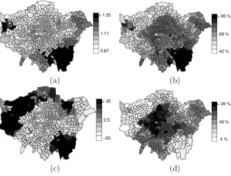
Lastly, Figure 7 examines the effects of PM10 on the probability of preterm birth and birth weight.

Figure 7 (a) displays the posterior medians of the area-wise log odds ratios of preterm birth when increasing the exposure to PM10 by one - the interquartile range of PM10. These are obtained by averaging over all

iterations the area specific odds ratios, exp(βi,11). We see that the model identifies a cluster in the SE and

a smaller one in the NW with higher odds of preterm birth. Estimates based on the model of Fern`andez & Green (2002) and the MCAR model exhibit similar behaviors, and hence corresponding results are not displayed. Figure 7 (b) displays the posterior probabilities thatβi,11are larger than zero: P(βi,11>0|data).

These are higher than 95% over the two aforementioned clusters of areas. Further, Figure 7 (c) displays the posterior means of βi,12. These describe the estimated effect of increasing exposure to PM10 by 1

µg/m3 on birth weight. Figure 7 (d) displays the posterior probabilities that βi,12 are less than zero:

P(βi,12<0|data). We see that the model identifies a group of areas in the central part of London for which

P(βi,12<0|data)>0.95. The corresponding estimated effects have posterior means not less than −20g.

6

Discussion

(a) (b)

(c) (d)

Figure 7: (a) Posterior medians of exp(βi,11) which represent odds ratio of preterm birth when increasing

exposure to PM10 by one - the interquartile range of PM10. (b) Posterior probabilities thatβi,11 are bigger

that zero, P(βi,11 > 0|data). (c) Posterior medians of βi,12, the coefficients of exposure to PM10 in the

model for birth weight. (d) Posterior probabilities that βi,12 are less that zero,P(βi,12<0|data).

estimation of the regression coefficients of interest. We have compared the proposed model, fi(yi,wi|xi) =

P∞

h=1πhif(yi,wi|xi;θh), to models of the form fi(yi|wi,xi) =

P∞

h=1πhif(yi|wi,xi;θ ∗

h) (Fern`andez &

Green, 2002; Green & Richardson, 2002), the more recent ones that take the form fi(yi,wi,xi) =

P∞

h=1πhig(yi|xi,wi;θ

0

h)h(xi,wi;θ

0

h) (Shahbaba & Neal, 2009; Hannah et al., 2011), some special cases

of the those and the more classical (M)CAR (Besag et al., 1991; Mardia, 1988) models. Our simula-tion studies have shown situasimula-tions in which the proposed model can do well in terms of estimating the underlying regression coefficients.

Computationally, the model we have proposed can be quite demanding, depending of course on the dimension and type of the variables included. There are two main steps in the MCMC algorithm, other than the updating of the GMRFs that is common to all models, that can be computationally intensive. Firstly, the numerical integration over the unobserved latent variables is numerically intensive and it can create numerical problems when integrating over latent variable distributions that correspond to empty clusters, as these sometimes can have covariance matrices that are close to being singular. However, we have chosen to perform the integration, instead of imputing the latent variables, as this greatly improves the mixing of the algorithm. Secondly, joint modeling of multivariate responses and confounders creates the need of handling possibly high dimensional covariance and precision matrices, which is also computationally demanding. Alternatively, one could impose diagonal covariance matrices, as in model M3that we examined

in the simulation study, but this option, in the scenario we examined, was not the best one in terms of RAMSE.

algorithm that excludes from the within cluster regression model risk factors that do not have an effect on the risk of the cluster is also of interest. Consider for instance a case similar to the one presented in the simulation studies, that is, a case where there is one count response variable, one risk factor, and one confounding variable. Further suppose that for most of the iterations of the sampler, two cluster are identified, for which linear predictors of the form ηh =β0h+β1hx, h= 1,2, adequately describe the within

cluster risk-risk factor relationship. Introduction now of a second confounding variable that contains no relevant information can potentially split the clusters into smaller ones. Of course, this will have a negative effect on the estimation of the within cluster regression coefficients. For instance, the second confounding variable could be a ‘coin flip’, meaning a binary variable that carries no information, that will split each of the two legitimate clusters into two smaller ones. Denote the new linear predictors as

ηhk = β0hk +β1hkx, h = 1,2, k = 1,2. Under this scenario, hypothesis tests of the form H0: β0h1 = β0h2,

and H0: β1h1 = β1h2, h = 1,2, will not be rejected with high probability. This can be the basis of

a variable selection algorithm suitable for the proposed model. Furthermore, continuing on the same example, exclusion of the within cluster risk factor can be performed in a straight forward way, based on hypothesis tests of the form H0: β1h = 0.

7

Acknowledgements

The authors thank the Medical Research Council (MRC) (grant number G09018401) for partially funding this research project, the Small Area Health Statistics Unit (SAHSU) and Anna Hansell of SAHSU, Imperial College London, for providing health, population, and birth data from Hospital Episode Statistics (HES) of the Health and Social Care Information Centre (HSCIC), and the Environmental Research Group, King’s College London, for providing the annual average exposure estimates of PM10. HES data are copyright

©2013, re-used with the permission of HSCIC. All rights reserved. The population and cancer data were supplied to SAHSU by the Office for National Statistics, derived from national cancer registrations and the Census. Data providing organizations did not participate in analysis or writing of this manuscript. Special thanks are due to Alex Beskos of University College London for his insightful discussion on the development of the MCMC sampler, and two anonymous referees for their insightful comments that have substantially improved this paper.

8

Appendix: MCMC algorithm

Our sampler utilizes the following steps:

1. Update ξ_h, h≥1, from

ξ_h| · · · ∼Nr3+q

 B

( X

i:δi=h

X∗_iTΣ∗_h−1vi+D−ξ1µξ

)

,B ≡

( X

i:δi=h

X∗_iTΣ_h∗−1X∗_i +D−_ξ1

)−1 .

2. To sample from the posterior of the restricted covariance matrix Σ∗_h, h ≥ 1, we use the parameter-extended algorithm of Zhang et al. (2006) that requires the joint posterior of (Dh,Σ∗h). This, apart

from a normalizing constant, is given by

p(Dh,Σ∗h|. . .)∝ |Dh|η/2−1|Σ∗h|

(η−s−1−nh)/2

etr{−(H−1Eh+Σ∗

−1

h Sh)/2},

where Sh =

P

Sampling at iteration t+ 1 proceeds as follows: given realizations from iteration t, D_h(t), Σ∗_h(t), we propose new values by generating E(_hp) ∼Wisharts(E(_hp);ψ,E(_ht)/ψ). Here, E(_ht) =D(t)

1/2

h Σ

∗(t)

h D

(t)1/2

h ,

and proposed values are obtained by decomposing E(_hp) = D(_hp)1/2Σ∗_h(p)D(_hp)1/2. Proposed values are accepted with probability

α= min

(

p(D(_hp),Σ∗_h(p)|. . .)

p(D(_ht),Σ∗_h(t)|. . .)

t(D(_ht),Σ_h∗(t)|D_h(p),Σ∗_h(p))

t(D(_hp),Σ∗_h(p)|D(_ht),Σ∗_h(t)),1

)

,

where, the proposal density is given byt(D(_hp),Σ_h∗(p)|D(_ht),Σ_h∗(t)) = Wisharts(E(_hp);ψ,E(_ht)/ψ)J(E(_hp) →

D_h(p),Σ_h∗(p)). We choose the degrees of freedomψso as to achieve an acceptance ratio of about 20−25% (Roberts & Rosenthal, 2001).

3. Vectors of regression coefficientsβ_h,1:2 = (βT_h1,βT_h2)T,h≥1, are updated from the marginal posterior, having integrated out y∗_i,1:2. We first partition vi = ((y∗i)T,wTi)T into unobserved and observed

variables vi = (y∗ T

i,1:2,sTi ). The distribution of vi, given in (4), is now re-written as

vi|(µ∗i,Σ ∗

i)∼Ns

 µ ∗ i =   0 0 µ_i,s  , Σ

∗

i =

Ri Fi

FT_i Gi

 .

The regression coefficients are updated from p(β_h,1:2|. . .)∝

Y

{i:δi=h}

hZ Ωi2

Z Ωi1

N2{y∗i,1:2|FhG−h1(si−µi,s),Rh −FhG−h1F T h}dy

∗ i,1:2

i

N(β_h1,β_h2;0, τ2I),

where Ωik = (ci,k,yi1−1, ci,k,yi1), k = 1,2.

At iteration t + 1, utilizing the realization from the previous iteration β(_h,t)_1:2, we propose a new value: β(_h,p)_1:2 = β(_h,t)_1:2 +, where ∼ N2r(0, τ2I). We choose τ2 in order to achieve acceptance

rate about 20−25% (Roberts & Rosenthal, 2001). The proposed value is accepted with probability

α = min{p(β(_h,p_1:2) |. . .)/p(β(_h,t)_1:2|. . .),1}. 4. Impute latent vectors y∗_i,1:2, i= 1, . . . , n,from

y∗_i,1:2 ∼N2(FhG−h1(si−µi,s),Rh−FhG−h1F T h)I[y

∗

i1 ∈Ωi1]I[y∗i2 ∈Ωi2]

using the algorithm described by Robert (2009), that is, by imputing one element of y∗_i,1:2 at a time given the other one.

5. Update the allocation variablesδi, i= 1,2, . . . , n,according to allocation probabilities obtained from

the marginalized posterior

P(δi =h)∝

hZ Ωi2

Z Ωi1

N2{y∗i,1:2|FhG−h1(si−µi,s),Rh−FhG−h1F T h}dy

∗ i,1:2

i

N1+q(si|µi,s,Gh)πhi.

6. Label switching moves (a generalization from Papaspiliopoulos & Roberts (2008)):

(a) Propose to change the labels a and b of two randomly chosen nonempty components. The proposed change is accepted with probability min1,Q

i:δi=a πbi πai

Q

i:δi=b πai πbi