Risk parameter estimation in volatility models

Risk-parameter estimation in volatility

models

Francq, Christian and Zakoian, Jean-Michel

4 October 2012

Online at

https://mpra.ub.uni-muenchen.de/41713/

models

Christian Francq

CREST and

University Lille 3 (EQUIPPE), BP 60149 59653 Villeneuve d’Ascq cedex, France e-mail:[email protected]

and

Jean-Michel Zakoïan

CREST, 15 Boulevard Gabriel Peri 92245 Malakoff Cedex, France

and

University Lille 3 (EQUIPPE) e-mail:[email protected]

∗

Abstract: This paper introduces the concept of risk parameter in con-ditional volatility models of the formǫt =σt(θ0)ηtand develops statis-tical procedures to estimate this parameter. For a given risk measure

r, the risk parameter is expressed as a function of the volatility co-efficients θ0 and the risk,r(ηt), of the innovation process. A two-step method is proposed to successively estimate these quantities. An alter-native one-step approach, relying on a reparameterization of the model and the use of a non Gaussian QML, is proposed. Asymptotic results are established for smooth risk measures as well as for the Value-at-Risk (VaR). Asymptotic comparisons of the two approaches for VaR estima-tion suggest a superiority of the one-step method when the innovaestima-tions are heavy-tailed. For standard GARCH models, the comparison only depends on characteristics of the innovations distribution, not on the volatility parameters. Monte-Carlo experiments and an empirical study illustrate these findings.

Keywords and phrases: GARCH, Quantile Regression, Quasi-Maximum Likelihood, Risk measures, Value-at-Risk.

∗_{We are grateful to the Agence Nationale de la Recherche (ANR), which supported}

1. Introduction

Modern financial risk management generally focuses on risks measures based on distributional information. Compared to traditional approaches relying on the marginal distribution of returns, more sophisticated approaches view risk as a stochastic process. For instance, conditional Value-at-Risk (VaR) - arguably the most widely used measure since the 1996 amendment of the Basel Capital Accord - is defined as the opposite of a quantile of the returns (or profit & losses, P&L, variables) conditional distribution. Another pop-ular risk measure is the conditional Expected Shortfall which, conditional on the past returns, measures the average loss when the loss is above the VaR1

. Many econometric approaches have been proposed in the finance and statistical literatures for measuring conditional risk.

A crucial issue that arises in this context is how to evaluate the perfor-mance of conditional risk estimators. Comparison of the perforperfor-mances of estimators of parameters based on the asymptotic theory is standard. But comparing the performances of VaR estimators, for instance, is more intricate because the conditional VaR is a random process, not a parameter.

The first objective of this paper is to introduce a concept ofrisk parameter

in conditional volatility models. The risk parameter can be interpreted as a summary of conditional risk. Summaries of unconditional risk (such as the VaR based on historical simulation) are commonly used but they do not account for the dynamics of risk. By contrast, risk parameters are vector coefficients which take into account the returns dynamics and for which an asymptotic theory of estimation can be derived.

To be more specific, consider a conditional volatility model of the form

ǫt=σt(θ0)ηt, (1.1)

where ǫt denotes the log-return,σt is a volatility process, that is a positive

measurable function of the past log-returns,θ0is a finite-dimensional

param-eter and (ηt) is a sequence of independent and identically distributed (iid)

random variables, ηt being also independent of the past returns. Consider a

risk measure, r, satisfying the assumption of positive homogeneity, such as the VaR or the Expected Shortfall. Then the conditional risk of ǫt is given

by

rt−1(ǫt) =σt(θ0)r(ηt),

1

where r(ηt) is a constant. In most parametric volatility models, multiplying

the volatility by a constant amounts to modifying the parameter value. Under this assumption, we have

rt−1(ǫt) =σt(θ0∗), where θ∗0 =H{θ0, r(ηt)} (1.2)

for some function H which is specific to the model under consideration. In this setting, we callθ₀∗therisk parameterassociated to the risk functionr. It incorporates not only the volatility parameters but also the (unconditional) risk of the innovation process(ηt). Whenris the risk associated with the VaR

at some levelα∈(0,1), the vectorθ₀∗ is referred to as theVaR parameter at levelα.

Deriving an asymptotic theory for estimators of risk parameters is the second objective of this article. Two estimation procedures will be studied and compared. A two-step approach relies on the expression of θ∗

0 in (1.2).

Under the identifiability assumption

Eη_t2= 1, (1.3)

a consistent and asymptotically normal (CAN) estimatorθˆof the parameter θ0can be obtained by standard methods for conditional volatility models, the

most widely used being the Gaussian Quasi-Maximum Likelihood (QML). In a second step, an estimatorrˆof the innovation riskr(ηt)can be constructed,

under conditions to be discussed, from the residualsηˆt=ǫt/σt(ˆθ)of the first

step. A consistent estimator H{θ,ˆ rˆ} of the risk parameter, θ₀∗, will be de-duced (under smoothness assumptions on the functionH). The asymptotic distribution of this estimator will follow from the joint asymptotic distribu-tion of{θ,ˆ rˆ}.

An alternative strategy of estimation introduced in this article relies on a reparameterization of the conditional volatility model. The multiplicative form of model (1.1) generally allows us to rewrite it as

ǫt=σt(θ∗0)η∗t, with r(ηt∗) = 1.

The latter equality replaces the standard assumption (1.3). The interest of such a representation is that, if a consistent estimator θˆ∗

0 of θ0∗ can be

ob-tained, the conditional risk rt−1(ǫt) of ǫt can be estimated in one step by

σt(ˆθ0∗).

In the framework of this paper, the condition r(η∗

t) = 1 is not necessarily

a moment condition. We propose a QML approach based on non-Gaussian densities depending on the risk functionr. A case of particular importance is the VaR at a given level α: the identifiability condition consists in setting an appropriate quantile of the distribution of η_t∗ to unity. It turns out that the only asymptotically valid QML criterion, that is, ensuring the consistency of the QML estimator of θ∗

0 whatever the distribution of ηt∗, takes the form of

a non linear quantile regression criterion.

The third objective of this article is to compare the one-step and two-step estimators of the VaR parameter. As we will see, the assumptions required for the CAN of the two estimators are quite different. When such assump-tions are met, the asymptotic variances can be compared. Surprisingly, for important subclasses of conditional volatility models the ranking of the two methods, in term of asymptotic efficiency, depends onα and on simple char-acteristics of the law of ηt, but not on the volatility parameter θ0.

Most of previous work on statistical inference for GARCH-type models dealt exclusively with the estimation of volatility parameters. The asymp-totic theory of the QML estimation for volatility parameters has been exten-sively studied, in particular for the GARCH(1,1) by Lee and Hansen (1994), Lumsdaine (1996), for the GARCH(p, q) by Berkes, Horváth and Kokoszka (2003) and Francq and Zakoïan (2004), for general models by Mikosch and Straumann (2006), Straumann and Mikosch (2006), Bardet and Winten-berger (2009). For the VaR parameter, it turns out that the QML criterion can be written under the form of a M-estimation criterion which is similar to those introduced in the quantile regression literature (see Koenker (2005) for a comprehensive book on quantile regression, and see Xiao and Koenker (2009), Xiao and Wan (2010) for recent applications to linear GARCH mod-els) and in the least-absolute deviations (LAD) time series literature (see Davis, Knight and Liu (1992), Davis and Dunsmuir (1997), Breidt, Davis and Trindade (2001), Ling (2005)).

The paper is organized as follows. In Section 2 we introduce the concept of risk parameter in a general conditional volatility model, and we discuss identifiability issues. Section 3 is devoted to the asymptotic properties of non-Gaussian QML estimators for general smooth risk measuresr. Section4

is devoted to the estimation of the VaR parameter. The smoothness assump-tions introduced in Section3being non satisfied by the VaR, the asymptotic properties of the one-step estimator are established in a completely different manner. The asymptotic properties of the two-step method are also estab-lished, and are compared with those of the one-step estimator. In Section

conditional Expected Shortfall. A Monte-Carlo study and applications on real financial data are provided in Section6. Section7concludes. Proofs are collected in the Appendix.

2. Risk parameter in volatility models

Most conditional volatility models are of the form

ǫt=σtηt

σt=σ(ǫt−1, ǫt−2, . . .;θ0) (2.1)

where (ηt) is a sequence of iid random variables, ηt being independent of {ǫu, u < t}, θ0 ∈ Rm is a parameter belonging to a parameter space Θ,

and σ : R∞×Θ → (0,∞). When Eηt = 0 and Eηt2 = 1, the variable

σ2

t is generally referred to as the volatility of ǫt. However, we will not make

such moment assumptions in this section and the following ones. A leading model, the most widely used among practitioners, is the GARCH(1,1) model of Engle (1982) and Bollerslev (1986), defined by

σ_t2=ω0+α0ǫ2t−1+β0σt2−1, (2.2)

where θ0 = (ω0, α0, β0)′ ∈ (0,∞)×[0,∞)×[0,1). For this model we have

σ2

t =

P∞

i=1β0i−1(ω0+α0ǫ2t−i), which is of the form (2.1).

It is assumed throughout that

A0: There exists a function H such that for any θ_∈Θ, for any K >0, and any sequence(xi)i

Kσ(x1, x2, . . .;θ) =σ(x1, x2, . . .;θ∗), where θ∗ =H(θ, K).

Most conditional volatility models are such that forK ≥1,θ∗≥θ componen-twise. For instance, in the GARCH(1,1) case we have θ∗ = (K2ω, K2α, β)′ with standard notation. The parameterθ0can thus be interpreted as a volatil-ity parameter in the sense that the largerθ0 the larger the volatility.

Now we define the notion ofrisk parameter. Following the terminology of Artzner, Delbaen, Eber, and Heath (1999), letrdenote a risk measure, that is, a mapping from the set of the real random variables to R. Assume that r is nonnegative, positively homogenous2

and law-invariant 3

. Then the risk ofǫt conditional on{ǫu, u < t}is given by

rt−1(ǫt) =σ(ǫt−1, ǫt−2, . . .;θ0)r(ηt). (2.3)

2

that is,r(λX) =λr(X)for any risk variableX and anyλ >0. 3

Now, assuming r(ηt)6= 0, let η∗t =ηt/r(ηt) and let θ0∗=H(θ0, r(ηt)). Under A0, the model can be reparameterized as

ǫt=σt∗ηt∗, r(η∗t) = 1,

σ∗

t =σ(ǫt−1, ǫt−2, . . .;θ0∗).

(2.4)

Because the conditional risk ofǫt is now simply

rt−1(ǫt) =σ(ǫt−1, ǫt−2, . . .;θ∗0),

θ∗

0 will be called the risk parameter.

Example 2.1(VaR parameter). An important example is the VaR, which

is the most standard risk measure used in the current regulations. For a continuous risk variable X with quantile function F_X−1, the VaR at level α, with α ∈ (0,1), is given by r(X) = −F_X−1(α). The conditional VaR of the process (ǫt) at risk levelα∈(0,1), denoted by VaRt(α), is defined by

Pt−1[ǫt<−VaRt(α)] =α,

where Pt−1 denotes the historical distribution conditional on {ǫu, u < t}.

When (ǫt) satisfies (2.1), the theoretical VaR is then given by

VaRt(α) =−σ(ǫt−1, ǫt−2, . . .;θ0)Fη−1(α)

whereFη is the probability distribution function ofηt. Letαbe small enough

so that F−1

η (α)<0. Thus (2.3) holds withrt−1(ǫt) = VaRt(α) and r(ηt) = −F_η−1(α). Now suppose that the volatility model is the GARCH(1,1) model (2.2). Then the VaR parameter at levelαis given byθ∗₀ = (K2ω0, K2α0, β0)′

withK =₋F−1

η (α). This coefficient takes into account the dynamics of the

GARCH process through the volatility parameters, but also the lower tail of the innovations distribution.

Example 2.2 (Expected Shortfall parameter). Another popular

mea-sure of financial risk is the expected shortfall (ES). One reason for its attractiveness is that, in contrast to the VaR, the ES satisfies the sub-additivity property (see Acerbi and Tasche (2002)). For a continuous risk variable X such that E(X−) < ∞, the ES at level α ∈ (0,1) is given by r(X) =₋E[X_|X _≤F_X−1(α)]. TheconditionalES of the process(ǫt) at risk

levelα, denoted by ESt(α), is defined by

Table 1

VaR and ES parameters at the 1% level for GARCH(1,1) models

Errors distribution ηt∼ N(0,1) ηt∼√1₂St4

Volatility parameter (1,0.05,0.9) (1,0.04,0.9) VaR parameter (5.41,0.27,0.9) (7.01,0.28,0.9) ES parameter (7.10,0.36,0.9) (13.63,0.55,0.9)

where Et−1 denotes the expectation conditional on {ǫu, u < t}. When (ǫt)

satisfies (2.1), the theoretical ES is then given by

ESt(α) =σ(ǫt−1, ǫt−2, . . .;θ0)ESη(α), (2.5)

where ESη(α) is the ES at level α of ηt, which is of the form (2.3).

For the GARCH(1,1) model (2.2), the ES parameter at level α is θ₀∗ = (K2ω0, K2α0, β0)′ withK =ESη(α).

Example 2.3 (VaR and ES parameters for two GARCH(1,1)). For

the sake of illustration, consider two GARCH(1,1) models with, respectively, standard Gaussian and standardized Student(4) innovations. The volatility parameter, as displayed in Table 1, is larger for the Gaussian-innovation model than for the Student-innovation model. In contrast, the VaR param-eter at level 1%is slightly larger for the second model. In other words, the first model is more volatile but less risky than the second one for the VaR at 1%. The difference between the two models is even more pronounced when ES-parameters at the level 1% are considered. In particular, the coefficient α∗

0, measuring the impact of a large squared return on the risk of the next

pe-riod, is 1.5 larger in the model with student errors than in the conditionally Gaussian model.

We consider estimating θ∗₀ by an appropriate QML method in the next section.

3. QML estimators of general risk parameters

In this section, we consider QML estimation of Model (2.4). The usual iden-tifiability condition Eη∗2

t = 1 being replaced by r(ηt∗) = 1, we will define a

non Gaussian QML estimator.

Given observationsǫ1, . . . , ǫn, and arbitrary initial values ǫ˜i for i≤0, we

define, under assumptions given below

˜

This random variable will be used to approximate

σt(θ) =σ(ǫt−1, ǫt−2, . . . , ǫ1, ǫ0, ǫ−1, . . .;θ).

We choose an arbitrary positive density h which can be called instrumental

density, and define the QML criterion

˜ Qn(θ) =

1 n

n

X

t=1

g(ǫt,σ˜t(θ)), g(x, σ) = log

1 σh

_x σ

. (3.1)

Let the QMLE

ˆ

θ_n∗ = arg max

θ∈Θ

˜

Qn(θ) (3.2)

for some compact subspaceΘofRm. This estimator is the standard Gaussian QMLE when h is the standard Gaussian density φ. However, the Gaussian QMLE is in general an inconsistent estimator of θ∗₀, unless if, for instance, the risk measure is r(X) =pE(X2_).

To derive the asymptotic properties of θˆ∗

n we introduce the following

as-sumptions.

A1: (ǫt) is a strictly stationary and ergodic solution of Model (2.4).

A2: For any real sequence (xi), the functionθ7→σ(x1, x2, . . .;θ) is

contin-uous. Almost surely,σt(θ)∈(ω,∞]for anyθ∈Θand for someω >0.

Moreover, σt(θ∗0)/σt(θ) = 1a.s. iffθ=θ∗0.

In addition, we assume that the function σ _→ Eg(η₀∗, σ) is valued in [_−∞,+_∞) and has a unique maximum at 1:

A3: Eg(η∗₀, σ)< Eg(η₀∗,1), ∀σ >0, σ6= 1.

A4: h is continuous on R, differentiable except on a finite set A, and there exist constants δ _≥ 0 and C0 > 0 such that for all u ∈ Ac,

|uh′(u)/h(u)| ≤C0(1 +|u|δ) withE|η∗0|δ <∞.Moreover, E|ǫ0|s <∞

for some s >0.

A5: There exist a random variableC1 measurable with respect to{ǫu, u <

0_} and a constant ρ_∈(0,1) such that sup_θ∈Θ|σt(θ)−σ˜t(θ)| ≤C1ρt.

Theorem 3.1 (Consistency of the risk parameter estimator). If

A0-A5 hold, then the QMLE defined by (3.1) and (3.2) satisfies

ˆ

The condition onh inA4 is mild; it vanishes for instance when the instru-mental density has the formh(u) =K1|u|λexp{K2|u|r}, for some constants

r, λ, K1, K2. In this case, the inequality is satisfied withδ =r. Assumptions

A2 and A5 can be simplified for specific forms of σt: for instance if the

model is a standard GARCH, A2 reduces to standard assumptions on the lag polynomials of the volatility andA5 can be directly verified. Note also that the only moment assumption on the observed process is the existence of a small moment inA4, which is automatically satisfied underA1in standard GARCH models.

We now discuss Assumption A3. Many risks measures involve a moment of a function of the risk variableX, in the sense that

r(X) = 1 iff E_{ψ(X)_}= 0 (3.3)

for some measurable function ψ :R → R. The following result shows that, for such risk measures,A3 can be omitted provided the QML instrumental density is appropriately chosen.

Proposition 3.1(Choice of the instrumental density). Letr(_·) satisfy-ing (3.3). AssumeA4 holds withA=∅. ThenA3holds for any distribution of η∗₀ satisfying r(η₀∗) = 1 iff the densityh is such that

x{logh(x)}′ = [λψ(x)−1], for all x (3.4)

and for some constantλ₆= 0.

This result provides a practical way to choose the QML density h, as illustrated in the next examples.

Example 3.1. Let r(X) = pE(X2_{). Then we have ψ(X) = 1−X}2 _and,

for any constantλ >0, by solving (3.4) we find

h(x)_{∝ |}x_|−(1−λ)exp(₋λx2/2). (3.5)

For λ= 1 the assumption A4 is satisfied and h is the density of the stan-dard Gaussian distribution. Thus, we retrieve the Gaussian likelihood for the standard identifiability conditionE(η_t∗2) = 1. It can be seen that any density hof the form (3.5) provides the same QMLE, it is thus not restrictive to take λ= 1.

Example 3.2. More generally, let r(X) =kXks = (E|X|s)1/s where sis a

X has an infinite second-order moment. In this case ψ(X) = 1_{− |}X_|s _and

we find , for λ >0 and for some constantc,

h(x)∝ |x|−(1−λ)exp(−λ|x|s/s). (3.6)

Forλ= 1, the assumption A4 is satisfied.

Example 3.3 (Example2.1continued). When the measure of risk is the VaR at level α, we have r(X) =₋F_X−1(α). Suppose that the distribution of the risk variableXis symmetric andα_∈(0,0.5). Thus (3.3) is satisfied with ψ(X) =1{|X|>1}−2α. Solving (3.4) yields

h(x) =hα(x) =λα(1−2α)|x|2λα−1{|x|−λ1{|x|>1}+1{|x|≤1}} (3.7)

for some positive constant λ. The choice of λ does not matter, any value leading to the sameθˆ_n∗. By choosing λ= (2α)−1, the density is defined onR

and satisfies A4. Since h is not differentiable everywhere, the assumptions of Proposition 3.1 are not satisfied. However, it will be shown in the next section that, under mild additional assumptions on the distribution of η0,

Assumptions A3 andA4 of Theorem3.1 hold true.

To show the asymptotic normality of θˆ∗

n we need additional

assump-tions which, for the reader’s convenience, are deferred to the appendix (see A6-A10 in Appendix A.1). Note that, for most classical GARCH for-mulations, A7 reduces to standard assumptions on lag polynomials and that A8 and A10 can be directly verified. Let g1(x, σ) = ∂g(x, σ)/∂σ,

g2(x, σ) =∂g1(x, σ)/∂σ.

Theorem 3.2 (Asymptotic normality). Under A0-A10 and if

Eg2(η∗0,1)6= 0 then

√

nθˆ_n∗₋θ∗_{0→ N}L (0,4τ_h,f2 I−1),

where

I =I(θ∗₀) =E

1 σ4

t

∂σ2_t ∂θ

∂σ2_t ∂θ′(θ

∗

0)

and τ_h,f2 = Eg

2 1(η0∗,1)

{Eg2(η0∗,1)}2

.

4. Estimating the conditional VaR

4.1. One-step VaR estimation

To estimate in one step the conditional VaR at levelα, as defined in Example

2.1, we first need to reparameterize Model (2.1). Ifα is not too large (more precisely α < P(η0 > 0)), from P[ηt < F−1(α)] = α we deduce P[η∗t < −1] = α where η_t∗ = −ηt/F−1(α). Letting θ0,α = θ∗0 = H(θ0,−F−1(α)),

under A0, the model can be reparameterized as

ǫt=σ∗tηt∗, P[ηt∗<−1] =α,

σ∗_t =σ(ǫt−1, ǫt−2, . . .;θ0,α). (4.1)

The theoretical VaR is now given by

VaRt(α) =σt(θ0,α). (4.2)

We will thus callθ0,α theVaR parameter at level α.

Define a QMLE ofθ0,α by

ˆ

θn,α = arg max θ∈Θ

n

X

t=1

log 1 ˜ σt(θ)

hα

ǫt

˜ σt(θ)

(4.3)

where hα is defined by (3.7). The following corollary of Theorem 3.1shows

that a one-step consistent estimator of the VaR parameter, not requiring any estimation of the quantile function of the innovationsηt, is given by

d

VaRt(α) = ˜σt(ˆθn,α). (4.4)

Corollary 4.1 (Consistency of the VaR parameter estimator). Let

(ǫt) be a strictly stationary and ergodic solution of (4.1), where the

distri-bution of η∗₀ is symmetric, satisfies the moment condition E_|log_|η₀∗_|| <_∞, and admits a density in a neighborhood of 1. If A0, A2 and A5 hold and if

E|ǫ0|s <∞ for some s >0, then, for all α∈(0,1/2), the QMLE defined by (4.3) satisfies

ˆ

θn,α →θ0,α, a.s.

Corollary 4.1it can be seen that

ˆ

θn,α = arg min θ∈Θ

1 n

n

X

t=1

log

|ǫt|

˜ σt(θ)

1{|ǫt|>˜σt(θ)}−2αlog

|ǫt|

˜ σt(θ)

= arg min

θ∈Θ

1 n

n

X

t=1

ρ1−2α

log

|ǫt|

˜ σt(θ)

. (4.5)

To interpret this expression, note that the first equation in Model (4.1) can be equivalently written as

log|ǫt|= logσ∗t + log|η∗t|, P[log|η∗0|<0] = 1−2α (4.6)

under the assumption of a symmetric distribution forη∗₀. Model (4.6) resem-bling a quantile regression model, it is not surprising to get an estimator of the form (4.5). An important difference with the quantile regression or au-toregression, however, is thatσ˜t(θ)is not assumed to be a linear combination

of explanatory variables, or past observables.

To study the asymptotic distribution of θˆn,α we need the following

addi-tional assumption.

A11: The density f∗ _{of η}∗

0 is continuous at 1 and satisfies f∗(1) > 0 and

M = sup_x∈R|x|f∗(x)<∞.

Theorem 4.1(Asymptotic normality). Under the assumptions of

Corol-lary 4.1, A6-A8 andA10-A11, there exists a sequence of local minimizers

ˆ

θn,α of the criterion defined in (4.5) satisfying

√

n(ˆθn,α−θ0,α)→ Nd

0,Ξα :=

2α(1₋2α) 4f∗2₍₁₎ J

−1

α

,

where Jα=EDt(θ0,α)Dt′(θ0,α) andDt(θ) =σt−1(θ)∂σt(θ)/∂θ.

LetΞbα denote a consistent estimator of the asymptotic variance Ξα. The

delta method thus suggests a(1−α0)%confidence interval forVaRt(α)whose

bounds are

˜

σt(ˆθn,α)±

Φ−₁₋1_α

0/2 √

n (

∂σ˜t(ˆθn,α)

∂θ′ bΞα

∂σ˜t(ˆθn,α)

∂θ

)1/2

, (4.7)

where Φ−_α01 denotes the α0-quantile of the standard Gaussian distribution.

4.2. Two-step VaR estimation

In this section, we consider the usual approach for estimating the VaR in Model (2.1) under the identifiability condition

Eη_t2= 1. (4.8)

This approach involves two steps. In a first step, the model is estimated by the standard QMLE and, in a second step, the theoretical quantileξα :=Fη−1(α)

is estimated using the estimated rescaled innovations. More precisely, letθˆn

denote the Gaussian QMLE ofθ0 in Model (2.1) under the constraint (4.8),

let

ˆ

ηt= ǫt

˜ σt(ˆθn)

,

and letξn,α denote the empiricalα-quantile ofηˆ1, . . . ,ηˆn.

An estimator of the VaR at level α is then given by

g

VaRt(α) =−σ˜t(ˆθn)ξn,α = ˜σt{H(ˆθn,−ξn,α)}

under A0 and provided ₋ξn,α > 0. A comparison of the VaR estimators

g

VaRt(α) andVaRdt(α) defined in (4.4) can then be based on the asymptotic

accuracies of the estimatorsθˆn,α and H(ˆθn,−ξn,α)of θ0,α.

Contrary to the one-step estimator, the resulting two step estimator of the VaR does not take advantage of the (hypothesized) symmetry of the errors distribution. An estimator exploiting this additional information is

g g

VaRt(α) = ˜σt(ˆθn)˜ξn,1−2α = ˜σt{H(ˆθn,ξ˜n,1−2α)}

where ξ˜n,1−2α is the empirical (1−2α)-quantile of |ηˆ1|, . . . ,|ηˆn|.

The next result gives the joint asymptotic distributions of(ˆθ′_n,−ξn,α)and

(ˆθ′_n,ξ˜n,1−2α).

Theorem 4.2. Assume ξα<0, Eη2t = 1 andκ4 :=Eηt4 <∞. Suppose that

η1 admits a density f in a neighborhood of ξα. Let A1, A5, A8 hold. Let A2, A6, A7 and A10 hold with δ= 2 andθ∗

0 replaced by θ0. Then

√

nθˆn−θ0

√

n(ξα−ξn,α)

! L

→ N(0,Σα), Σα=

_κ4−1

4 J−1 λαJ−1Ω

λαΩ′J−1 ζα

,

where Ω =E(Dt), J =E(DtD′t) with Dt=Dt(θ0), and

λα = ξα

κ4−1

4 +

pα

2f(ξα)

, ζα=ξ2α

κ4−1

4 +

ξαpα

f(ξα)

+α(1−α) f2_(ξ

α)

0.0 0.2 0.4 0.6 0.8 1.0

0

2

4

6

8

α

Asymptotic v

ar

iances

0.0 0.2 0.4 0.6 0.8 1.0

0

1

2

3

α

Asymptotic v

ar

iances

Fig 1_. Asymptotic variances _ζα in dotted lines, and _α(1−_α)/f2_(ξα) in full line,

for a standard Gaussian distribution (left panel) and the standardized GED(ν) with

ν = 0.25(right panel).

with pα=E η211{η1<ξα}

−α.

Under the additional assumption that η1 is symmetrically distributed, we have

√ n

_ˆ

θn−θ0

˜

ξn,1−2α+ξα

L

→ N(0,Σ˜α), Σ˜α =

κ4−1

4 J−1 −λαJ−1Ω

−λαΩ′J−1 ζ˜α

where

˜ ζα =ξα2

κ4−1

4 +

ξαpα

f(ξα)

+2α(1−2α) 4f2_(ξ

α)

=ζα−

α 2f2_(ξ

α)

.

Remark:The asymptotic variance ζα of the empirical quantile of the

stan-dardized residualsηˆtis the sum ofα(1−α)/f2(ξα), which can be interpreted

as the asymptotic variance of the empiricalα-quantile of theηt’s, and a term

due to the estimation of θ0,α. The same additional term appears inζ˜α.

Un-expectedly, this term measuring the effect of estimation can be negative. For instance, for a standard Gaussian distribution we have

ξ2_ακ4−1

4 +

ξαpα

f(ξα)

= −1 2 ξ

2

α≤0.

We now deduce the asymptotic distributions of thetwo-stepand the sym-metric two-step estimators θˆ2_n,αS :=H(ˆθn,−ξn,α) and θˆn,αS2S :=H(ˆθn,ξ˜n,1−2α)

ofθ0,α=H(θ0,−ξα).

Corollary 4.2. Under the assumptions of Theorem 4.2, the two-step esti-mators of the VaR-parameter at levelα satisfy

√

nθˆ_n,α2S −θ0,α

_L

→ N(0,Υα), √n

ˆ

θS_n,α2S−θ0,α

_L

→ N(0,Υ˜α),

where

Υα=

∂H(θ, ξ) ∂(θ′_{, ξ)}

(θ0,−ξα) Σα

∂H(θ, ξ) ∂(θ′_{, ξ)}′

(θ0,−ξα) ,

andΥ˜α is obtained by replacing Σα by Σ˜α in Υα.

It can be noted that, because the matricesΣ˜α andΣα only differ by their

lower-right term, with ξα > ξ˜α, we have, in the sense of positive definite

matrices,

˜

ΥαΥα.

Thus, the symmetric two-step estimator is asymptotically more accurate than the two-step estimator. But the former estimator is inconsistent if the errors distribution is not symmetric.

4.3. Comparing the one-step and two-step estimators in the standard GARCH case

The results of Theorem 3.1 are now applied to the standard GARCH(p, q)

model

ǫt=σtηt,

σ_t2=ω0+Pq_i=1α0iǫ2_t−i+Pp_j=1β0jσ_t2_−j, (4.9)

where θ0 = (ω0, α01, . . . , β0p)′ satisfies ω0 >0, α0i ≥0, β0j ≥0.Let

θ0 = θ [1:q+1] 0

0p

!

, θ₀[1:q+1]= (ω0, α01, . . . , α0q)′, A=

ξ_α2Iq+1 0

0 Ip

.

Corollary 4.3. Under the assumptions of Corollary 4.2, for the standard GARCH model (4.9) the asymptotic variances of the two-step estimators of the VaR parameter take the form

Υα =

κ4−1

4 A{J

−1_−4θ 0θ

′

0}A+ 4ξα2

α(1₋α) f2_(ξ

α)

θ0θ

′

0,

˜ Υα =

κ4−1

4 A{J

−1_−4θ 0θ

′

0}A+ξα2

2α(1−2α) f2_(ξ

α)

θ0θ

′

To compare the asymptotic variances of the two estimators of θ0,α note

that

J_α−1=AJ−1A, fη∗(1) =−ξ_αf(ξ_α). Hence

Varas{√n(ˆθn,α−θ0,α)}=

2α(1−2α) 4ξ2

αf2(ξα)

AJ−1A.

It follows that

Varas{√n(ˆθn,α−θ0,α)} −Υα = ∆αA

J−1

4 −θ0θ ′

0

A₋ 2α ξ2

αf2(ξα)

Aθ0θ′0A′,

Varas{√n(ˆθn,α−θ0,α)} −Υ˜α = ∆αA

J−1

4 −θ0θ ′

0

A,

where

∆α=

2α(1₋2α) ξ2

αf2(ξα) −

(κ4−1). (4.10)

The following result is a consequence of the fact that 4θ0θ

′

0 J−1. It

allows to compare the asymptotic variances of the one-step estimator θˆn,α

and two-step estimator θˆS2S n,α.

Corollary 4.4. Under the assumptions of Corollary 4.2, for the standard GARCH model (4.9) with symmetric innovations, we have

Varas{√n(ˆθn,α−θ0,α)} Varas

n_√

nθˆ_n,αS2S−θ0,α

o

iff ∆α≤0.

Interestingly, comparing the asymptotic variance matrices of the estima-tors amounts to determining the sign of a real coefficient, which solely de-pends on the distribution of ηt. None of the methods is superior in every

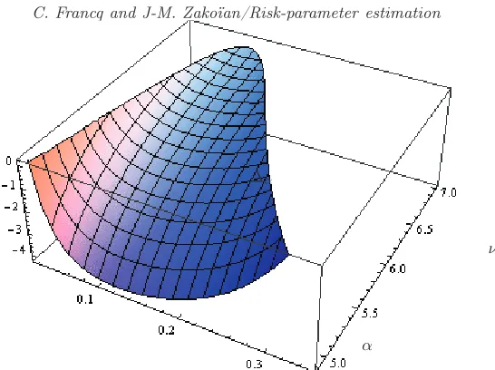
situation. If the fourth-order moment is large, a fortioriif it does not exist, the one-step estimator will be better. Conversely, for distributions admitting moments at any order (such as the Gaussian) the two-step estimator may be superior. Figure 2 shows the surface ∆α ≤ 0, as a function of α and

ν, for Student distributions with ν degrees of freedom. It can be seen that for small and moderate values of ν, the one-step estimator is asymptotically more efficient than the two-step estimator for the values of αwhich are used in practice. In Figure 3, ∆α is drawn as a function of ν, for GED(ν) and

∆α

ν

α

Fig 2_{.Surface∆α≤0, with∆α defined in (4.10), for which the one-step estimator}

is asymptotically more efficient than the symmetric two-step estimator ofθ0_,α when

the distribution ofηtis a standardized Student withν degrees of freedom,ν∈[4.9,7]

andα∈[0.01,0.35].

0.0 0.1 0.2 0.3 0.4 0.5

0

1

2

3

ν ∆α

α =0.01

α =0.05

0.0 1.0 2.0 3.0

−80

−60

−40

−20

0

ν ∆α

α =0.01

α =0.05

Fig 3_{.∆α, defined in (4.10), forα∈ {0.01,0.05}, when the distribution ofηtfollows}

5. Extensions

5.1. One-step estimation of the VaR parameter without the symmetry assumption

We have seen that, under the assumption that the distribution ofη₀∗ is sym-metric and under some regularity assumptions, the VaR parameter θ0,α

de-fined by (4.2) is consistently estimated by a QMLE, if and only if the instru-mental densityh is that defined by (3.6). This estimator has the form of the quantile estimator θˆn,α defined by (4.5) in the nonlinear regression model

(4.6), but may be inconsistent when the distribution of η∗

0 is asymmetric.

It is however possible to define a one-step quantile estimator of the VaR parameter without assuming that η∗₀ is symmetric. To this aim, note that similarly to (4.6) we have forǫt<0

logǫ−_t = logσ_t∗+ logη∗−_t , P[logη∗−_t <0_|ǫt<0] =τ0

where x− = max{0,−x} and τ0 = 1− {α/P(η∗t < 0)}. This leads us to

consider the quantile estimator

˘

θn,α = arg min θ∈Θ

X

t:ǫt<0 ρˆτ

log

ǫ−_t ˜ σt(θ)

, τˆ= 1₋ 1 n

n

X

t=1

1l_{ǫt<0} !−1

α.

It is known (see Lemma 2.3 in Berkes, Horváth and Kokoszka, 2003) that any strictly stationarity GARCH model possesses a fractional moment of order s_∈(0,1). It is then easy to check that for these models the following assumption holds true.

A13: Esup_θ∈Θ|logσ1(θ)|<∞.

Theorem 5.1. Let(ǫt) be a strictly stationary and ergodic solution of (4.1),

where the distribution of η₀∗ satisfies Elog+η∗−₀ <∞, and admits a density in a neighborhood of -1. If A0, A2, A5 and A13 hold, then, for all α ∈

(0, P(η∗

0 <0)), we have

˘

θn,α →θ0,α, a.s.

where θ0,α is the VaR parameter satisfying (4.2).

The asymptotic distribution of this estimator is left for future research.

5.2. Two-step estimation of the ES parameter

this reason, ES estimation is not amenable to the one-step QML estima-tion method developed in Secestima-tion3. However, the two step approach can be derived as follows.

Let µα = −E(η0 | η0 < ξα) denote the ES of the distribution of η0. By

(2.5) andA0, the theoretical ES is given by

ESt(α) =σ(ǫt−1, ǫt−2, . . .;θ0)ESη(α) =σ(ǫt−1, ǫt−2, . . .;θ∗0,α), (5.1)

where θ∗

0,α=H(θ0, µα) is the ES parameter at levelα.

An estimator ofθ∗_0,α is then given by

f

ESt(α) = ˜σt(ˆθn)µn,α= ˜σt{H(ˆθn, µn,α)}

where µn,α is the ES of the errors:

µn,α =−

Pn

t=1ηˆt1lηˆt<ξn,α Pn

t=11lηˆt<ξn,α

= −1

[nα] + 1

n

X

t=1

ˆ

ηt1lηˆt<ξn,α,

andH(ˆθn, µn,α) is an estimator of the ES parameter.

The next result gives the joint asymptotic distribution of (ˆθ′_n, µn,α), and

the asymptotic distribution of H(ˆθn, µn,α) in the standard GARCH case.

Theorem 5.2. Assumeµα >0,Eηt2 = 1andκ4 :=Eηt4 <∞.Let A1,A5, A8 hold. Let A2, A6, A7 and A10hold with δ = 2 andθ∗

0 replaced by θ0. Then

√

nθˆn−θ0

√

n(µn,α−µα)

! L

→ N(0,Γα), Γα =

_κ4−1

4 J−1 ϕαJ−1Ω

ϕαΩ′J−1 να

,

where J is as in Theorem 4.2and

να=σα2 +

κ4−1

4 µ

2

α+µαxα, ϕα=−

1

2xα−µα κ4−1

4 ,

σ_α2 = 1

α2var{(ηt−ξα)1lηt<ξα}, xα= 1 αcov

1₋η_t2,(ηt−ξα)1lηt<ξα .

It follows that the asymptotic distribution of the ES parameter is given by

√

n(H(ˆθn, µn,α)−θ0∗,α) d

→ N 0,

∂H(θ, µ) ∂(θ′_{, µ)}

(θ0,µα) Γα

∂H(θ, µ) ∂(θ′_{, µ)}′

(θ0,µα) !

.

For the standard GARCH model (4.9), we have

√

n(H(ˆθn, µn,α)−θ∗0,α) d

where

Υ∗_α = κ4−1

4 A

∗_{J−1_−4θ

0θ′0}A∗+ 4µα2σα2θ0θ′0,

and A∗ _{is obtained by replacing ξ}

α by µα inA.

The asymptotic distribution of the ES-parameter estimator thus depends on the GARCH coefficients and simple characteristics of the innovations distribution. In contrast with the VaR parameter, the asymptotic variance does not involve the density of the errors distribution and thus can be more straightforwardly estimated. In the asymptotic variance να of the errors ES

estimator, the term σ2_α can be interpreted as the asymptotic variance of the ES estimator if theηt’s were observed (see Chen, 2008). The additional term,

κ4−1

4 µ2α+µαxα, thus reflects the effect of estimating the GARCH coefficients.

6. Numerical experiments

A Monte Carlo study was conducted in order to throw light on the perfor-mance of the VaR-parameter estimators in finite sample. We also report an empirical application to stock indices.

6.1. On simulated data

We begin by considering one of the simplest volatility model, the ARCH(1) where ηt follows the Student distribution withν degrees of freedom:

ǫt=σtηt, σt2=ω0+α0ǫ2t−1, ηt∼Stν. (6.1)

In this model, the VaR parameter is equal toθ0,α= (ω0,α, α0,α)whereω0,α=

ω0Kν2,α0,α=α0Kν2, and Kν denoted the α-quantile of the Stν. Simulating

N = 1, 000 independent trajectories of size n = 500 and n = 5,000 of this model, we compared the estimations of θ0,α obtained by the one-step

estimator θˆn,α and the two-step estimator θˆSn,α2S. We considered the VaR

levelsα= 0.01andα= 0.05. The intercept was fixed toω0 = 1and we took

α0 = exp(−Elogη21)/5, which guarantees strict stationarity of the model

for any value of ν (the necessary and sufficient strict stationarity condition being Elogα0η21 < 0). Over the N simulations, and for both components

of θ0,α, the root mean squared error of estimation of the two methods are

respectively denoted byRMSE1 andRMSE2. We then defined the empirical

Table 2

ERE of the one-step method with respect to the two-step method for estimating the VaR parameter for the ARCH(1) model with Student innovations (6.1). The number of replication isN= 1,000, the level of the VaR isα= 5%orα= 1%and the length of

each simulation isn= 500orn= 5,000.

n= 500 n= 5,000

ν ν

1 2 3 4 5 6 ∞ 1 2 3 4 5 6 ∞

α= 5%

ω0,α 7.5 2.8 1.7 1.3 1 0.9 0.9 13.9 6.6 2.7 1.3 1.1 1 0.8 α0,α 7.3 3.6 1.7 1.3 1 1.0 0.8 22.2 8.7 3.2 1.3 1.1 1 0.9

α= 1%

ω0,α 6.1 1.6 1.0 0.8 0.7 0.7 0.7 41.1 3.6 1.6 0.9 0.8 0.8 0.7 α0,α 3.8 1.8 2.6 0.8 0.7 0.7 0.7 13.7 6.0 2.1 0.9 0.8 0.7 0.7

one-step method can be considered as twice more efficient than the two-step method. Table6.1shows that, as expected from the asymptotic theory, the estimator θˆn,α is much more accurate than θˆ2n,αS when the distribution

of ηt is heavy-tailed (i.e. ν is small) whereas θˆn,α2S is slightly more accurate

than θˆn,α when the distribution of ηt is close to the normal (i.e. ν is large).

Similar conclusions were obtained for other distributions of the noise and for more elaborate volatility models. In particular, we considered the Threshold GARCH model introduced by Zakoïan (1994)

ǫt=σtηt, σt=ω0+α0+ǫ+t−1+α0−ǫ−t−1+β0σt−1, ηt∼GED(ν). (6.2)

The VaR parameter is now θ0,α = (ω0,α, α0+,α, α0−,α, β0) where ω0,α = −ω0Kν, α0+,α = −α0+Kν, α0−,α = −α0−Kν, and Kν denotes the α

-quantile of the GED(ν). In our simulation experiments, we choseω0 = 0.001,

β0 = 0.87,α0+=α/4andα0−=αwhereαis such thatElog(α|ηt|+β0) = 0,

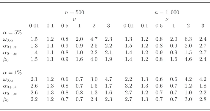
which ensures a strict stationary solution to (6.2). The results presented in Table3are in accordance with Figure 3. The one-step estimator of the VaR parameter is more accurate then the two-step estimator when ν ≤ 0.1 or whenνis large (depending on the value ofα). In the Gaussian case (ν = 0.5), the two-step method should be preferred.

6.2. On real data

Table 3

ERE of the one-step method with respect to the two-step method for estimating the VaR parameter for the TGARCH(1,1) with GED(ν) innovations (6.2). The number of replication isN= 1,000, the level of the VaR isα= 5%orα= 1%and the length of

each simulation isn= 500orn= 1,000.

n= 500 n= 1,000

ν ν

0.01 0.1 0.5 1 2 3 0.01 0.1 0.5 1 2 3

α= 5%

ω0,α 1.5 1.2 0.8 2.0 4.7 2.3 1.3 1.2 0.8 2.0 6.3 2.4

α0+,α 1.3 1.1 0.9 0.9 2.5 2.2 1.5 1.2 0.8 0.9 2.0 2.7

α0−,α 1.4 1.1 0.8 1.0 2.2 2.1 1.4 1.2 0.9 0.9 1.5 2.7

β0 1.5 1.1 0.9 1.6 4.0 1.9 1.4 1.2 0.8 1.6 4.6 2.4

α= 1%

ω0,α 2.1 1.2 0.6 0.7 3.0 4.7 2.2 1.3 0.6 0.6 4.2 4.2

α0+,α 2.6 1.3 0.8 0.7 1.5 1.7 3.2 1.3 0.6 0.7 1.2 1.8

α0−,α 2.6 1.3 0.8 0.8 1.3 1.6 2.7 1.2 0.7 0.7 1.0 2.2

β0 2.2 1.2 0.7 0.7 2.4 2.3 2.7 1.3 0.7 0.7 3.0 2.8

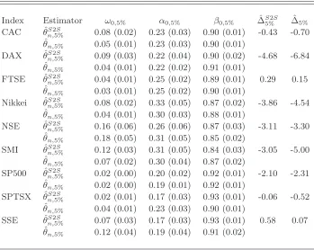
(London), Nikkei (Tokyo), NSE (Bombay), SMI (Switzerland), SP500 (New York), SPTSX (Toronto), and SSE (Shanghai). For each series of log-returns, ǫt= log(pt/pt−1) where pt denotes the value of the index, we estimated the

VaR parameterθ0,αof GARCH(1,1) models, forα= 5%and 1%. We report

in Table 4 our estimates of θ0,α obtained by the one-step and the

symmet-ric two-step methods, along with standard deviations. We also report two estimates of ∆α based on residuals ηˆt or ηˆ∗t of the two-step or the one-step

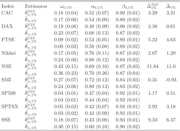
method. Such estimates are negative for 7 out of 9 indices indicating, by Corollary 4.4, a superiority in accuracy of the one-step method for the risk level 5%. The conclusions are quite different when more extreme risks are considered. Table5shows that, forα= 1%, the two-step method is probably more efficient than the one-step method for large n (except perhaps for the SMI).

Table 6 reports estimation results for the ES parameter. While the esti-mated VaR parameters over the nine stocks were very similar, large differ-ences between stocks appear when risk is measured by the ES. In particular, the Nikkei, NSE and SMI display much larger estimated ARCH coefficients α_0,5% andα_0,1%.

Table 4

One-step estimatorθˆn,α and two-step estimatorθˆSn,α2S for the VaR parameterθ0,αat level α= 5%of GARCH(1,1) models for 9 stock market indices. The estimated standard deviations are given into brackets. The last two columns displays estimations of∆α (θˆn,α

should be asymptotically more efficient thanθˆS2S

n,α if and only if∆α<0) based on

residuals of the two-step and one-step methods.

Index Estimator ω0,5% α0,5% β0,5% ∆ˆS5%2S ∆ˆ5%

CAC θˆSn,25%S 0.08 (0.02) 0.23 (0.03) 0.90 (0.01) -0.43 -0.70 ˆ

θn,5% 0.05 (0.01) 0.23 (0.03) 0.90 (0.01)

DAX θˆSn,25%S 0.09 (0.03) 0.22 (0.04) 0.90 (0.02) -4.68 -6.84 ˆ

θn,5% 0.04 (0.01) 0.22 (0.02) 0.91 (0.01)

FTSE θˆS2S

n,5% 0.04 (0.01) 0.25 (0.02) 0.89 (0.01) 0.29 0.15 ˆ

θn,5% 0.03 (0.01) 0.25 (0.02) 0.90 (0.01)

Nikkei θˆSn,25%S 0.08 (0.02) 0.33 (0.05) 0.87 (0.02) -3.86 -4.54 ˆ

θn,5% 0.04 (0.01) 0.30 (0.03) 0.88 (0.01)

NSE θˆSn,25%S 0.16 (0.06) 0.26 (0.06) 0.87 (0.03) -3.11 -3.30 ˆ

θn,5% 0.18 (0.05) 0.31 (0.05) 0.85 (0.02)

SMI θˆSn,25%S 0.12 (0.03) 0.31 (0.05) 0.84 (0.03) -3.05 -5.00 ˆ

θn,5% 0.07 (0.02) 0.30 (0.04) 0.87 (0.02)

SP500 θˆS2S

n,5% 0.02 (0.00) 0.20 (0.02) 0.92 (0.01) -2.10 -2.31 ˆ

θn,5% 0.02 (0.00) 0.19 (0.01) 0.92 (0.01)

SPTSX θˆS2S

n,5% 0.02 (0.01) 0.17 (0.03) 0.93 (0.01) -0.06 -0.52 ˆ

θn,5% 0.04 (0.01) 0.23 (0.03) 0.90 (0.01)

SSE θˆSn,25%S 0.07 (0.03) 0.17 (0.03) 0.93 (0.01) 0.58 0.07 ˆ

θn,5% 0.12 (0.04) 0.19 (0.04) 0.91 (0.02)

26, 2011. The(1−α0)%confidence intervals (forα0= 5%) are obtained from

formula (4.7). We preferred to report the opposite of the VaR, because the aim of such risk measures is to determine the capital reserve which acts as a protection against big losses (i.e.large negative values of ǫt). Obviously the

Table 5

As Table4but for the risk levelα= 0.01

Index Estimator ω0,1% α0,1% β0,1% ∆ˆS1%2S ∆ˆ1%

CAC θˆS2S

n,1% 0.18 (0.04) 0.52 (0.07) 0.90 (0.01) 3.29 3.31 ˆ

θn,1% 0.17 (0.06) 0.54 (0.09) 0.89 (0.02)

DAX θˆn,S21%S 0.19 (0.06) 0.48 (0.09) 0.90 (0.02) 2.38 0.61 ˆ

θn,1% 0.23 (0.07) 0.68 (0.13) 0.87 (0.02)

FTSE θˆn,S21%S 0.09 (0.02) 0.53 (0.05) 0.89 (0.01) 5.22 4.63 ˆ

θn,1% 0.08 (0.03) 0.58 (0.08) 0.89 (0.02)

Nikkei θˆn,S21%S 0.17 (0.05) 0.76 (0.11) 0.87 (0.02) 2.07 1.20 ˆ

θn,1% 0.24 (0.06) 0.88 (0.12) 0.84 (0.02)

NSE θˆS2S

n,1% 0.42 (0.15) 0.69 (0.16) 0.87 (0.03) 11.84 11.0 ˆ

θn,1% 0.36 (0.23) 0.70 (0.26) 0.87 (0.04)

SMI θˆS2S

n,1% 0.27 (0.07) 0.72 (0.12) 0.84 (0.03) 0.31 -0.93 ˆ

θn,1% 0.24 (0.06) 0.80 (0.13) 0.83 (0.02)

SP500 θˆn,S21%S 0.04 (0.01) 0.47 (0.04) 0.92 (0.01) 1.17 0.51 ˆ

θn,1% 0.04 (0.01) 0.44 (0.04) 0.92 (0.01)

SPTSX θˆn,S21%S 0.05 (0.02) 0.42 (0.07) 0.93 (0.01) 2.92 3.18 ˆ

θn,1% 0.03 (0.02) 0.42 (0.09) 0.93 (0.01)

SSE θˆn,S21%S 0.18 (0.07) 0.43 (0.08) 0.93 (0.01) 9.33 6.47 ˆ

θn,1% 0.30 (0.15) 0.60 (0.16) 0.90 (0.02)

Table 6

Estimation of the ES parameter of GARCH(1,1) models at levelα= 5%andα= 1%for 9 stock market indices. The estimated standard deviations are given into brackets.

Index ω∗

0,5% α∗0,5% β0∗,5% ω0∗,1% α∗0,1% β∗0,1%

Retur

n and −V

aR

−8

−6

−4

−2

0

2

4

2011−08−08

Fig 4_{. Returns, estimated -VaR (at the 5% and 1% levels) and VaR accuracy}

in-tervals for the SP index from April, 6, 2011 to August, 26, 2011. Estimation of the VaR parameter is based on the 500 previous values.

7. Conclusion

This paper presented two methods for estimating the risk parameter in con-ditionally heteroskedastic models. Asymptotic results were established for general risk measure, and a particular attention was devoted to the VaR and the ES.

The introduction of a VaR parameter facilitates the asymptotic compari-son of the risk evaluation procedures. In particular, for the standard GARCH models the ranking of the two methods, in terms of asymptotic relative effi-ciency, only depends on the sign of the scalar∆αdefined by (4.10), involving

Retur

n and −ES

−8

−6

−4

−2

0

2

4

2011−08−08

Fig 5_{.Returns, estimated ES (at the 5% and 1%levels) and ES accuracy intervals}

for the SP index from April, 6, 2011 to August, 26, 2011. Estimation of the ES parameter is based on the 500 previous values.

turns out that the asymptotic distribution of the estimator depends on the GARCH coefficients and other simple characteristics of the innovations dis-tribution.

Finally, the estimation risk, namely the effect of the inaccuracy of the parameter estimation on the risk evaluation, can be explicitly taken into account, leading to confidence bounds for the VaR and the ES.

Appendix A: Technical assumptions and proofs

A.1. Technical assumptions

A6: θ∗

0 belongs to the interior ofΘ.

A7: There exist no non-zerox_∈Rmsuch thatx′∂σt(θ0∗)

∂θ = 0, a.s.

A8: The functionθ_7→σ(x1, x2, . . .;θ)has continuous second-order derivatives, and

sup θ∈Θ

∂σt(θ) ∂θ −

∂σ˜t(θ) ∂θ +

∂2_σ

t(θ) ∂θ∂θ′ −

∂2_σ˜

t(θ) ∂θ∂θ′

≤

C1ρt,

whereC1andρare as inA5.

A9: his twice differentiable with_|u2_(h′_(u)/h(u))′

| ≤C0(1 +|u|δ)for allu∈R. A10: There exists a neighborhood V(θ∗

0) of θ∗0 such that the following variables have

finite expectation:

sup θ∈V(θ∗

0) 1 σt(θ)

∂σt(θ) ∂θ 4 , sup θ∈V(θ∗

0) 1 σt(θ)

∂2_σ

t(θ) ∂θ∂θ′ 2 , sup θ∈V(θ∗

0)

σt(θ∗0)

σt(θ)

2δ .

A.2. Proofs for the results of Section 3

We start by a lemma. Forx/σ_∈Ac_{, let}

g1(x, σ) =

∂g(x, σ) ∂σ =−

1 σ−

h′_(x/σ)

h(x/σ) x σ2.

Lemma A.1. Under AssumptionA4, forσ,σ > ω >˜ 0we have, forσ⋆_{betweenσ andσ˜}

such thatx/σ⋆ ∈Ac_,

|g(x, σ)₋g(x,σ˜)_{| ≤}







|g1(x, σ⋆)||σ−σ˜| ifx6= 0, 1

ω|σ−σ˜| ifx= 0.

Proof. It is not restrictive to assume σ > ˜σ. For x = 06 , write A ∩(x/σ, x/˜σ) = {x/σ1, . . . , x/σj} when this set is non empty. By convention, j = 0 when this set is empty. Assume

σ=σ0> σ1> . . . > σj+1= ˜σ.

By applying Rolle’s theorem on the sets(x/σi, x/σi+1)we get, forσ⋆i ∈(σi, σi+1),

|g(x, σ)₋g(x,σ˜)_|=

j X i=0

g1(x, σi⋆)(σi+1−σi)

≤sup i |

g1(x, σi⋆)|(σ−σ˜).

We also have|g(0, σ)−g(0,˜σ)|= logσ−log ˜σand the conclusion follows.

Proof of Theorem3.1.The consistency is a consequence of the following intermediate results (seee.g.the proofs of Theorem 7.1 in Francq and Zakoian, 2010):

i) lim n→∞supθ∈Θ|

Qn(θ)−Q˜n(θ)|= 0, a.s.

ii)E|g(ǫt, σt(θ∗0))|<∞ and ifθ6=θ0∗, Eg(ǫt, σt(θ))<Eg(ǫt, σt(θ0∗)),

iii)anyθ₆=θ∗

0 has a neighborhoodV(θ)such that

lim sup n→∞

sup θ∗_∈V(θ)

˜

Qn(θ∗)< lim n→∞

˜

where

Qn(θ) = 1 n

n

X

t=1

g(ǫt, σt(θ)).

LetK be a generic positive constant, allowed to be a random variable, measurable with respect to_{ǫu, u≤0}, whose values will be modified along the proofs.

We begin by showingi). Using a Taylor expansion, almost surely sup

θ∈Θ|

Qn(θ)−Q˜n(θ)|

≤ n−1 n

X

t=1

sup θ∈Θ|

g1(ǫt, σ⋆t(θ))||σ˜t(θ)−σt(θ)|1{ǫt6=0}

+n−1 n

X

t=1

sup θ∈Θ

1

ω|σ˜t(θ)−σt(θ)|1{ǫt=0}

≤ n−1K n

X

t=1

ρtsup θ∈Θ 1 σ⋆ t ǫt σ⋆ t h′ h _ǫ t σ⋆ t

1_{ǫt6=0}+K ω n −1 n X t=1 ρt

≤ Kn−1 n

X

t=1

ρt(1 +_|ǫt|δ),

where g1 is defined in Theorem 3.2and σt⋆(θ) is between σ˜t(θ) and σt(θ).The first in-equality is a consequence of Lemma A.1. The last two inequalities rest on Assumptions

A2,A4andA5. By the Markov inequality andA4, we deduce

∞ X

t=1

P(ρt_|ǫt|δ> ε) ≤ ∞ X

t=1

ρts/δ

E|ǫt|s εsδ

<_∞

and thus ρt

|ǫt|δ → 0 a.sby the Borel-Cantelli lemma. Thus, i) follows by the Cesàro lemma.

Conditionii)is a consequence of A2-A3. Indeed,

E{g(ǫt, σt(θ))−g(ǫt, σt(θ0∗))}=E

g

ηt∗, σt(θ) σt(θ∗0)

−g(ηt∗,1)

≤0,

with equality iffθ=θ∗0.

The proof ofiii)is omitted because it uses more standard arguments.

Proof of Proposition 3.1.First assume thathsatisfies (3.4). By AssumptionsA4and

A2, the function σ 7→ ∂logh(η0∗/σ)∂σ is bounded by an integrable random variable,

uniformly in a neighborhood of any σ >0. By the dominated convergence theorem, we thus have

∂ ∂σEg(η

∗

0, σ) = −

1 σ − 1 σE λψ

η∗0

σ

−1

,

which is equal to zero if and only if r(η0∗/σ) = 1. By r(η0∗) = 1 and by the positive

homogeneity ofr,r(η∗

0/σ) = 1is equivalent toσ= 1. Thus, forhsatisfying (3.4),A3is

a consequence of (3.3).

To prove the "only if" part, note that

A3 _{⇒ E}

h′_(η∗

0)

h(η∗

0)

η0∗

Note also thatψcannot be null onRbecause this would implyr(X) = 1for any variable

X, by (3.3), in contradiction with the positive homogeneity of r. Now if (3.4) does not hold, then for somex1, x2withψ(x1)6= 0, andλ16=λ2

h′(xi) h(xi)

xi+ 1 =λiψ(xi), i= 1,2.

Letηsuch thatP(η=xi) =pi>0withp1+p2= 1, andψ(x1)p1+ψ(x2)p2 = 0.Then

Eψ(η) = 0and

E

h′(η) h(η)η

+ 1 =λ1ψ(x1)p1+λ2ψ(x2)p2= (λ1−λ2)ψ(x1)p16= 0.

Then, in view of (A.1), AssumptionA3is not satisfied. We have found a distribution of

η0∗such thatr(η0∗) = 1butA3is not satisfied. The proposition follows.

Proof of Theorem3.2.The proof is based on a Taylor expansion of the criterionQ˜nat θ∗

0. Sinceθˆn∗ converges toθ∗0, which stands in the interior of the parameter space byA6,

fornlarge enough the derivative of the criterion is equal to zero atθˆ∗n. We thus have

0 = √n n

X

t=1

∂

∂θg(ǫt,σ˜t(θ

∗

0)) +

1 n n X t=1 ∂2

∂θi∂θj

g(ǫt,σ˜t(θ∗ij))

!

√

nθˆ∗n−θ∗0

where theθ∗ij’s are betweenθˆ∗nand θ0∗. The asymptotic normality is proven by means of

the following intermediate results: for some neighboorhoodV(θ∗

0)ofθ∗0,

iv) lim n→∞

√_{n sup} θ∈V(θ∗

0) ∂

∂θQn(θ)− ∂ ∂θQ˜n(θ)

= 0, in probability,

v) ∂

2

∂θ∂θ′Qn(θ

∗_)→ Eg2(η∗0,1)

4 I , in probability,

vi)√n∂ ∂θQn(θ

∗

0)→ NL

0,Eg

2 1(η∗0,1)

4 I

,

vii)I is nonsingular,

for anyθ∗_betweenθˆ∗

nandθ0∗. For brevity, we will skip the proof ofv)-vii)which is available

from the authors. To proveiv)we note that sup

θ∈V(θ∗

0) √_n ∂

∂θQn(θ)− ∂ ∂θQ˜n(θ)

≤ sup θ∈V(θ∗

0) 1 √ n n X t=1

|g1(ǫt, σt(θ))−g1(ǫt,σ˜t(θ))|

∂σt(θ) ∂θ + sup θ∈V(θ∗

0) 1 √_n n X t=1

|g1(ǫt,σ˜t(θ))|

∂σt(θ) ∂θ −

∂˜σt(θ) ∂θ . (A.2)

Note that_|g1(ǫt,σ˜t(θ))| ≤K(1 +|ǫt|δ) byA4and the first part ofA2. Thus, using A8, the last term in (A.2) is bounded by

K √_n

n

X

t=1

It is not restrictive to assumes < δinA4. We have, by thecr-inequality,

E

∞ X

t=1

ρt(1 +_|ǫt|δ)

!s/δ

≤ ∞ X

t=1

ρst/δ(1 +_|ǫt|s)<∞.

It follows that

K √_n

n

X

t=1

ρt(1 +|ǫt|δ)≤√K n

∞ X

t=1

ρt(1 +|ǫt|δ)→0, a.s.

Thus the second term in the right-hand side of (A.2) goes to 0a.s.

The first term in (A.2) is bounded by

sup θ∈V(θ∗

0) 1 √_n n X t=1

|g2(ǫt, σ∗t(θ))|Kρt

∂σt(θ) ∂θ (A.3)

whereg2(x, σ) =∂g1(x, σ)/∂σandσt∗(θ)is betweenσ˜t(θ)andσt(θ).Noting that

g2(x, σ) = 1

σ2

1 +x σ 2h ′ h + x σ h′ h ′ x σ , we have

|g2(ǫt, σ∗t(θ))| ≤ K σ∗

t(θ)

1 +|ǫt|δ

byA4,A9and the first part ofA2. The term in (A.3) is thus bounded by

K √_n

n

X

t=1

ρt(1 +|ǫt|δ) sup θ∈V(θ∗

0) 1 σt(θ)

∂σt(θ) ∂θ .

By the Cauchy-Schwarz inequality andA10we have, fors <2δ,

E

∞ X

t=1

ρt(1 +_|ǫt|δ) sup θ∈V(θ∗

0) 1 σt(θ)

∂σt(θ) ∂θ

!s/2δ

≤   ∞ X t=1

ρst/2δ{E(1 + 2|ǫt|s/2+|ǫt|s)}1/2

(

E sup θ∈V(θ∗

0) 1 σt(θ)

∂σt(θ) ∂θ

s/δ)1/2

<∞.

We can conclude that the first term in the right-hand side of (A.2) goes to 0a.s., which

completes the proof ofiv).

A.3. Proofs for the results of Section 4

Proof of Corollary 4.1.The distribution ofηt∗being symmetric, first note that Model (4.1) is in the form (2.4) withr(η∗

t) =Fη−∗1(1−α). Thus A1is satisfied. Now note that

ˆ

θn,α= ˆθ∗n, whereθˆ∗nis defined by (3.1)-(3.2) with, up to an additive constant,g(ǫt,σ˜t(θ)) equal to

AssumptionA4being satisfied with A={−1,0,1}and δ = 0, it remains to show that

A3holds true and the conclusion will follow from Theorem3.1. Note thatE_|g(η∗

0,1)|<∞under the moment condition onlog|η∗0|. Moreover, for any

σ >0, σ₆= 1, the distribution ofη∗

0 being symmetric,

Eg(η∗0, σ)−Eg(η∗0,1) =−λE(log|η∗0| −logσ)(1{|η∗

0|>σ}−1{|η0∗|>1})≤0.

Note that the inequality is strict becauseη0∗ admits a density in a neighborhood of 1,

which completes the proof.

Proof of Theorem4.1.First note thatνˆn:=√n(ˆθn,α−θ0,α)is such that

ˆ

νn= arg min ν∈Λn

˜ Sn(ν),

whereΛn:=√n(Θ−θ0,α)and

˜ Sn(ν) =

n

X

t=1

ρ1−2α

log

|ǫt| ˜

σt(θ0,α+n−1/2ν)

−ρ1−2α

log

|ǫt| ˜ σt(θ0,α)

.

Showing that the initial values are asymptotically negligible, and linearizinglogσt(θ0,α+ n−1/2_{ν)aroundν= 0, LemmaA.2below demonstrates thatS˜}

n(ν)can be approximated by

Sn(ν) = n

X

t=1

ρ1−2α

log|ηt∗| − ν′

√_nDt(θ0,α)

−ρ1−2α(log|ηt∗|).

Let flog|η∗_| denote the density of the variable log|η∗t|. Using a convexity argument, LemmaA.3then shows thatSn(ν)weakly converges to the process

S(ν) =p2α(1₋2α)ν′N+flog|η∗|(0)ν′Jαν/2, N ∼ N(0, Jα).

The process is minimized at

ˆ ν=₋

p

2α(1₋2α) flog|η∗_|(0)

Jα−1N ∼ N 0,

2α(1₋2α) f2

log|η∗_|(0)

Jα−1

!

The conclusion follows from Remark 1 and Lemma 2.2 in Davis, Knight and Liu (1992).

Lemma A.2. Let_CK ={ν ∈Rm:kνk ≤ K}. Under the assumptions of Theorem 4.1,

for allK >0, we have

sup ν∈CK

|Sn(ν)−S˜n(ν)|=oP(1).

Proof:LetD˙t(θ) = _∂θ∂Dt′(θ), and letD˜t(θ)(resp.D˙˜t(θ)) be obtained by replacingσt(θ) byσ˜t(θ)inDt(θ)(resp.D˙t(θ)). A Taylor expansion yields

log ˜σt

θ0,α+ ν √_n

= log ˜σt(θ0,α) +

1 X

i=0

˜ vt,n(i)(ν),

with

˜ v(0)t,n(ν) =

1

√_nν′D˜t(θ0,α), v˜t,n(1)(ν) = 1 2nν

whereθ˜∗t is betweenθ0,αandθ0,α+n−1/2ν. Letη˜t=ǫt/˜σt(θ0,α). Using the identity

ρ1−2α(u−v)−ρ1−2α(u) = ₋v(1₋2α₋1_{u<0}) + (u₋v)

1_{0>u>v}−1_{0<u<v}

= ₋v(1₋2α₋1_{u<0}) +

Z v

0

1_{u≤s}−1_{u<0} ds (A.4)

foru6= 0(see Equation (A.3) in Koenker and Xiao, 2006), we obtain

˜ Sn(ν) =

1 X

i=0

˜

Tn(i)(ν) + ˜Un(i)(ν),

with

˜

Tn(i)(ν) = − n

X

t=1

˜

vt,n(i)(ν)(1−2α−1{|η˜t|<1}),

and

˜ Un(0)(ν) =

n

X

t=1

˜

ξt,n(0)(ν), ξ˜

(0)

t,n(ν) =

Z v˜(0)_t,n(ν)

0

1_{log|η˜

t|≤s}−1{log|η˜t|<0} ds,

˜ Un(1)(ν) =

n

X

t=1

˜

ξt,n(1)(ν), ξ˜

(1)

t,n(ν) =

Z P1_i=0v˜(t,ni)(ν)

˜

v_t,n(0)(ν)

1_{log|η˜

t|≤s}−1{log|η˜t|<0} ds.

Define Tn(i)(ν) by replacingσ˜t(·) byσt(·) in T˜n(i)(ν). Define Un(i)(ν), ξt,n(i)(ν) and v

(i)

t,n(ν) similarly. Noting thatTn(1)(ν)is centered and has a variance of orderO(1/n)uniformly in ν, in view ofA10, we obtainsup_ν∈CK|Tn(1)(ν)|=oP(1). Now we have

˜

Tn(1)(ν)−Tn(1)(ν)

≤ 1 2n n X t=1 ν

′_D˙˜ t(˜θt∗)ν

1 ∗

{|ǫt|∈(σt(θ0,α),σ˜t(θ0,α))} + 1 2n n X t=1 ν

′n_D˙˜

t(˜θ∗t)−D˙t(˜θ∗t)

o

ν

with1∗

{X∈(a,b)}=1{X<b}−1{X<a}for any real numbersa, band any real random variable

X. The second term of the right-hand side of the previous inequality is bounded by

KPn

t=1ρ

t_{/n=o(1)byA2,A5andA8. Using the Hölder inequality,A10, and}

E 1

∗

{|ǫt|∈(σt(θ0,α),σ˜t(θ0,α))} ≤P

|ηt∗| ∈

1,σt(θ0,α) ˜ σt(θ0,α)

≤Kρt (A.5)

the first term also tends to zero. Thussup_ν∈CK|T˜n(1)(ν)|=oP(1).Furthermore

T˜

(0)

n (ν)−Tn(0)(ν)

≤ 1 √_n n X t=1 ν

′_D˜ t(θ0,α)

1 ∗

{|ǫt|∈(σt(θ0,α),σ˜t(θ0,α))}

+_√1 n n X t=1 ν ′n ˜

Dt(θ0,α)−Dt(θ0,α)

o

Now, using the elementary relation

Z ˜a

0

˜ f(x)dx₋

Za

0

f(x)dx=

Z ˜a

a ˜ f(x)dx+

Z a

0 n

˜

f(x)₋f(x)odx

with standard notations, we have

|ξ˜t,n(0)(ν)−ξ

(0)

t,n(ν)|=

Zv˜(0)_t,n(ν)

v(0)_t,n(ν)

1_{log|η˜

t|≤s}−1{log|η˜t|<0} ds

+

Z vt,n(0)(ν)

0 (

1∗ {|η∗

t|∈

es_,es˜σt(θ0,α) σt(θ0,α)

}− 1∗

{|η∗ t|∈

1,σt_σt˜(₍θ_θ0,α) 0,α) } ) ds .

Using the inequalities√n_|v_t,n(0)(ν)₋v˜(0)_t,n(ν)_{| ≤}Kρt _{and (A.5), splitting the latter integral} into two parts, and taking conditional expectation, we then obtain

Et−1|ξ˜t,n(0)(ν)−ξ

(0)

t,n(ν)| ≤ Kρt

√_n +

Z 1 n1/4

0

Kρtds+ 2|vt,n(0)(ν)|1_{|v(0)

t,n(ν)|≥n−1/4}

whereEt−1 denotes the expectation conditional on{ηu:u < t}. Using in particular

E_|v(0)_t,n(ν)_|1

{|v_t,n(0)(ν)|≥n−1/4_} ≤

ν′Dt(θ0,α)/√n

4

n

P(_|ν′Dt(θ0,α)| ≥n1/4)

o3/4

≤ K/n11/16,

the Markov inequality shows thatsup_ν∈CK|U˜n(0)(ν)−Un(0)(ν)|=oP(1).Similarly, one can show thatsup_ν∈CK|U˜n(1)(ν)−Un(1)(ν)|=oP(1).

Now note that

Et−1ξ

(1)

t,n(ν)

≤

Z P1_i=0v(t,ni)(ν)

v(0)_t,n(ν)

Z s

0

flog|η∗_|(s)ds ≤

Z P1_i=0v(t,ni)(ν)

v(0)t,n(ν)

smax

[0,s] |flog|η∗|(x)|ds.

ByA11and arguments already given, the expectation of the previous variable is of order

OP(n−3/2). It follows thatsupν∈CK|U (1)

n (ν)|=oP(1). We have thus shown that

sup ν∈CK

|S˜n(ν)−Tn(0)(ν)−Un(0)(ν)|=oP(1).

The conclusion follows by noting that, in view of (A.4),Sn(ν) =Tn(0)(ν) +Un(0)(ν).

Lemma A.3. Under the assumptions of Theorem4.1 we have Sn(·)→d S(·)

Proof:We have shown in LemmaA.2that (A.4) entails

Sn(ν) =Tn(ν) +Un(ν),

with

Tn(ν) =− ν′ √ n n X t=1

Dt(θ0,α)(1−2α−1{|η∗ t|<1})

and

Un(ν) = n

X

t=1

ξt,n(ν),

ξt,n(ν) =

log_|η∗t| − ν′

√_nDt(θ0,α)

×

1

{√ν′_nDt(θ0,α)<log|η∗t|<0}− 1

{√ν′_nDt(θ0,α)>log|ηt∗|>0}

.

We have

Et−1

log_|ηt∗| − ν′

√_nDt(θ0,α)

1

{ν′

√_nDt(θ0,α)>log|η∗t|>0}

= 1 {ν′

√_nDt(θ0,α)>0}

Z √ν_n′Dt(θ0,α)

0

x−√ν′_nDt(θ0,α)

flog|η∗_|(x)dx

= flog|η∗_|(0)1

{ν′

√_nDt(θ0,α)>0}

Z √ν′_nDt(θ0,α)

0

x−√ν_n′ Dt(θ0,α)

dx+Rn,t

= −1

2nflog|η∗|(0)1{ν′

√_nDt(θ0,α)>0}ν ′_D

t(θ0,α)D′t(θ0,α)ν+Rn,t

whereRn,tis equal to

1

{√ν′_nDt(θ0,α)>0}

Z √ν′_nDt(θ0,α)

0

x₋ ν

′

√_nDt(θ0,α)

(flog|η∗_|(x)−flog|η∗_|(0))dx.

By A11, for any ǫ > 0 there exists τ > 0 such that _|x_| < τ entails _|flog|η∗_|(x)−

flog|η∗_|(0)|< ǫ. It follows that

|Rn,t| ≤ 1 2n{ν

′_D

t(θ0,α)}2(ǫ+ 2M1_{ν′

√_nDt(θ0,α)>τ}).

By the Hölder and Markov inequalities andA10, we then show thatPn

t=1|Rn,t|=o(1)

a.s.Similarly,

Et−1

log_|η∗t| − ν′

√_nDt(θ0,α)

1

{√ν′_nDt(θ0,α)<log|η∗t|<0}

= 1

2nflog|η∗|(0)1{√ν′_nDt(θ0,α)<0}ν ′_D

t(θ0,α)Dt′(θ0,α)ν+R∗n,t

whereR∗

n,tis analogous toRn,t. We thus have

n

X

t=1

Et−1ξt,n(ν) = flog|η∗_|(0)

1 2n

n

X

t=1

ν′Dt(θ0,α)D′t(θ0,α)ν+o(1)