JN METD2 A Fortran IV Programme for Solving Neutron Transport Problems with Isotropic Scattering in Multilayer Slabs by the jN Method EUR 4839

FORTRAN-IV PROGRAMME FOR SOLVING . " Ώ Ρ

NEUTRON TRANSPORT PROBLEMS

4

^ ^ p | ^ ^ | w ^

WITH ISOTROPIC SCATTERING IN MULTILAYER

Nuclear Studies Division

assume any liability with respect to the use of, from the use of any information, apparatus, me in this document.

i»f

'?ifcp

!

Í

¿

ff.

« w i l

or for damages resulting method or process disclosed

8

This report is on sale at the addresses listed on cover page 4

β Ι

ι

1

P « i % i i i « S

at the price of B.Fr. 85.—

lir

fm,

!

IJi

D.G

29,

July 1972

"'•''^¡5ιΐιΐι· Η· li.'. ·* ι « * Sti ì'.iiiuiif !''3B«J

4M

_{ocument was reproduced on the basis of the best av}

Ä8

document

i!

i

_Mili

sm

Wßm

Silli

EUR 4839 e

JN-METD2 - A FORTRAN-IV PROGRAMME FOR SOLVING NEUTRON TRANSPORT PROBLEMS WITH ISOTROPIC SCATTERING IN MULTILAYER SLABS BY THE j ^ METHOD by T. ASAOKA and E. CAGLIOTI BONANNI

Commission of the European Communities

Joint Nuclear Research Centre - Ispra Establishment (Italy) Nuclear Studies Division

Luxembourg, July 1972 - 58 Pages - B.Fr. 85.—

The mathematical formulae of the jjy method for the description of neutron transport in a multilayer slab system are summarized within the context of a multigroup model under the assumption that the scattering of neutrons is spherically symmetric in the laboratory system. A Fortran-IV computer programme JN-METD2 is described in detail for the use of accurately solving the transport problem according to these formulae. The computer code calculates the eigenvalue of the integral transport equation, the effective multiplication factor or the asymptotic decay constant of neutrons, as well as the eigenfunction, the space, angle and energy dependent flux distribution. In addition, it evaluates the first three time moments of the time-dependent flux resulting from a delta function boundary source with space, angle and energy variables.

EUR 4839 e

JN-METD2 - A FORTRAN-IV PROGRAMME FOR SOLVING NEUTRON TRANSPORT PROBLEMS WITH ISOTROPIC SCATTERING IN MULTILAYER SLABS BY THE jN METHOD by T. ASAOKA and

E. CAGLIOTI BONANNI

Commission of the European Communities

Joint Nuclear Research Centre - Ispra Establishment (Italy) Nuclear Studies Division

Luxembourg, July 1972 - 58 Pages - B.Fr. 85.—

The mathematical formulae of the jjy method for the description of neutron transport in a multilayer slab system are summarized within the context of a multigroup model under the assumption that the scattering of neutrons is spherically symmetric in the laboratory system. A Fortran-IV computer programme JN-METD2 is described in detail for the use of accurately solving the transport problem according to these formulae. The computer code calculates the eigenvalue of the integral transport equation, the effective multiplication factor or the asymptotic decay constant of neutrons, as well as the eigenfunction, the space, angle and energy dependent flux distribution. In addition, it evaluates the first three time moments of the time-dependent flux resulting from a delta function boundary source with space, angle and energy variables.

EUR 4839 e

JN-METD2 - A FORTRAN-IV PROGRAMME FOR SOLVING NEUTRON TRANSPORT PROBLEMS WITH ISOTROPIC SCATTERING IN MULTILAYER SLABS BY THE j ^ METHOD by T. ASAOKA and E. CAGLIOTI BONANNI

Commission of the European Communities

Joint Nuclear Research Centre - Ispra Establishment (Italy) Nuclear Studies Division

Luxembourg, July 1972 - 58 Pages - B.Fr. 85.—

E U R 4 8 3 9 e

COMMISSION OF THE EUROPEAN COMMUNITIES

JN-METD2

A FORTRAN-IV PROGRAMME FOR SOLVING

NEUTRON TRANSPORT PROBLEMS

WITH ISOTROPIC SCATTERING IN MULTILAYER

SLABS BY THE j

N

METHOD

by

T. ASAOKA and E. CAGLIOTI BONANNI

1972

Joint Nuclear Research Centre Ispra Establishment - Italy

programme JN-METD2 is described in detail for the use of accurately solving the transport problem according to these formulae. The computer code calculates the eigenvalue of the integral transport equation, the effective multiplication factor or the asymptotic decay constant of neutrons, as well as the eigenfunction, the space, angle and energy dependent flux distribution. In addition, it evaluates the first three time moments of the time-dependent flux resulting from a delta function boundary source with space, angle and energy variables.

KEYWORDS

FORTRAN

1-DIMENSIONAL CALCULATIONS TRANSPORT THEORY

PLATES ZONES NEUTRONS ISOTROPY SCATTERING

EIGENVALUES

NEUTRON SPECTRA

MULTIPLICATION FACTORS TIME DEPENDENCE

C O N T E N T S

page

1. Introduction 5

2. Mathematical Formulae 6

3. JN­METD2 Computer Code 11

3.1 Input data 11

3.2 Computer programme 15

4. Remarks 1 θ

Table I 20

Table II 21

References 22

Appendix 1. Analytical Expressions of Functions 25

i. J

tr

(0¡¡,tf¿,xj;

I)

23

2

· Fp(flr¿,fyF,/M;eO

5S

3. £,(#,<*,·,5, J ; < 0

39

Appendix 2. Flow Diagrams of Computer Programmes 48

1. MAIN 4&

2. JNMETD 49

3. FLUXCA 5'

JN-METD2, A FORTRAN-IV PROGRAMME FOR SOLVING NEUTRON TRANSPORT PROBLEMS WITH ISOTROPIC SCATTERING IN MULTILAYER SLABS BY THE j METHOD

N

1. Introduction

Under the assumption that the scattering of neutrons is spherically symmetric in the laboratory system, the newly developed j method has already yielded accurate solutions to space-energy time-dependent transport problems in bare spheres (ASAOKA, 1968-1) and space-angle energy-time dependent problems in homogeneous slabs (ASAOKA, 1968-2). The neutron flux for a stationary state has also been obtained as a simple limiting case of time-dependent problems. For dealing with these problems, a computer code JN-METD1 has been developed within the context of the multigroup and (up to) j approximation (ASAOKA,1971),

As already shown by several authors, the approach can easily be extended to take into account anisotropic scattering of neutrons (KSCHWENDT, 1971) or to treat multilayer slab systems (MANGIAROTTI, 1971). For the description of time-dependent neutron transport in multilayer slabs with anisotropic scat-tering, a general formalism has been developed by the present authors (ASAOKA and CAGLIOTI, 1969 and 1972) and applied to an optimization study of moderators in pulsed reactors. Furthermore, the application of the method to convex geo-metries has been demonstrated for a homogeneous medium in which the neutron scattering is isotropic (HEMBD, 1970).

The present report is concerned with the computer code JN-METD2 designed to solve transport problems in multilayer slab systems with isotropic scattering of neutrons. By the use of a multigroup model and the j (N^7) approximation, the computer code calculates :

(a) The space, angle and energy dependent neutron flux due to a stationary point-isotropic boundary source, as well as the first and second time moments of the time-dependent flux resulting from a point-isotropic delta function source on one boundary.

(c) The asymptotic decay constant of the fundamental neutron distribution in a multilayer slab system.

2. Mathematical Formulae

Since a general formulation for time­dependent transport in multilayer slabs with anisotropic scattering has already been shown in a previous paper (ASAOKA and CAGLIOTI, 1972), we only summarize here the mathematical formulae for the description of neutron transport in a M­region slab within the context of a G­energy­group model and the j approximation (scattering being assumed sphe­

rically symmetric).

Let X be the space coordinate, JU the direction cosine of the neutron velo­ city, 2Γ«1 and I/, the macroscopic total cross section of the i­th region (ex­ tending from 3C=s d^^ to d¿ ) and the speed of neutrons in the g­th group, re­ spectively, and CiC3­>?) the mean number of secondary neutrons produced in the g­th group as a result of collisions in the g'­th group and i­th region. The number of the g­th group neutrons in tne j­tn region resulting from a point­isotropic delta function source Sa {fXM,^)= 2$aJA %(%) $l~tl can be written as

ti

+ ^ ) ^ a r ^ ­ r v 4 ¿ 2 >+^F,(## få* ,/,x/tA­zv^; |*­*­

(1)

where 0f?­¿= ζ * ^ * ^ " ^ ) ΐ ?^-\' {^VcA)/(T^V* ) } , Z V stands for the

7 ­

-00 '

χ y*

2

$

w

ä'jwf

Ï-PJa-Lz/ï-t'l

.

The function Γρ i s equal to Fp£ with /=£? evaluated previously (ASAOKA and CALGIOTI, 1972). The explicit expression for rp in the j approximation

( p £ 7 ) is given in the Appendix 1, Section 2. In addition, À^T^^JÍJk and υ _ι( ^7 -AJÍ") i n equation (1) are respectively a pole and the residue of

'Vpi (?; A") which satisfies the following linear equation:

+

| W>|

0

té, *r(#f' ^-¿«

ΆΦ·

1

)VAM>*

where

( 4 )

χ

fajufi-rjt'ifaMtf

( Í P J ^ ) .

(5)

The explicit expressions for the integrals £<«# and Je«, are respectively shown in the Appendix 1, Sections 4 and 1.

in which

(9)

the expression for Cr» being given in the Appendix 1, Section 3.

It is seen from equation (6) that the critical condition for a system with­ out extraneous source Sa = O is to be obtained by solving the determinantal equation:

^ - i < M )

u^M»**·-«**^

> )

= 0.

­ 9 ­

In order to get the value of the effective multiplication factor k

^

Λ

for a

eff

given reactor,

Ci

O f ­ ^ f O *­

s

divided into two parts. These are the scat­

tering part

Ç

i

i(j->1')=zJc3->3

/

)/JSj*

and

t h e

fission part Cf'Cg­^g'^s

= X./(V2f)e^/JS·^

where %« stands for the proportion of fission neutrons

born in the $~th group. By the use of this separation, the value of

k is

obtained by solving equation (10) with

The ratios between B y

(9")

S can now be obtained, under the condition (10),

from equation (6) with

Sa=0

and

Cl(9->3')

given by equation (11) for calcula­

ting the flux distribution in

a multilayer slab reactor according to equation

(7) or (8) with

Sa~0

. In addition, equation (10) with

¿d-XjtyJj

instead

of Zy'lfy

gives the asymptotic decay constant

\ = jtftyU'Jf)

which governs

the asymptotic behaviour of neutrons as t­>&) {"see equation (1)J .

It is also easy to get the time moments of the time­dependent flux resulting

from the incidence of an external delta function source on one boundary:

$»(X,IÅjtl~ 2SiU%iX)S(.'t^

·

T h e

first three time moments of

the angu­

lar flux (1) are written as follows:

/^^α,/,Ο^^α,/ο,

­00 (12)

which i s given by equation (7) with R, (*p=

-Vp

(f/2f*lfy}

£ compare equation

(3) with ( 6 ) J .

)

o

<tt i*v.n

ê

kz,ju

}

t )=2 S

%

x

x

s4f [­(¡g

z

a

%-^+^hx-ßj^l^l^^jif+

Φ>& % ψ,

^^-4^)V<^> W,

.

(14

According to equation (3), the first and second derivatives of ­#. (í}>>¿) a t •4 = 2"//lfy a r e obtained by solving respectively the following equations:

^!*(ΐ«ί*-*^*·'))Λ^)ΐ}.

* (16) For a non-multiplying system in which there is no up-scattering of neutrons,

equations (3) [or (6)} , (15) and (16) can be simplified to those which are solved in the same way as for a one-group model. For example, equation (3) can be reduced to

11

-From equations (12)-(14), the first three time moments of the total flux can be obtained as follows:

given by equation (8), (18)

(19)

(20)

3. JN-METD2 Computer Code

3.1 Input data_(see the Appendix 3)

After a title card with a 20A4 format, 16 integers are read with a 2513 for-mat. These input integers are defined as follows:

H O 3, 5 or 7 for the j , j or j approximation (0 to stop the

execu-tion; see the Appendix 2, Section 1)

IIII 0 for solving a new problem or 1 for restarting a problem for

NSOUCE NSLOWD IGRP IHT IHS JHL NSPH NNNN LLL IAA NENRGY NTFLUX

­1, 0 or 1 for the problem to obtain the asymptotic decay constant (NSPH=1 and LLL=0; if NSL0WD=1 the decay constant of neutrons be­ longing to the lowest energy­group being calculated), to compute the value of the effective multiplication factor (NSLOWD=0 and NSPH=1) or to deal with a subcriticai system with an external source for obtaining the flux distribution

1 for non­multiplying system without up­scattering of neutrons (0 otherwise)

Total number of energy groups

Arrangement of reaction type of the cross section (XSEC) for the g­th group and i­th region; XSEC (l,g,i) = ΣΑ*1 ,..., XSEC(IHT­1,

g,i) = Xu , XSEC (IHT>3,g,i) = Ztrf > XSEC (IHT+l,g,i) = Z'<g+IHS­IHT­>g),,..., XSEC (IHS­l,g,i) = ZLl(g+l­»g), XSEC (IHS^IHT,g,i) = Z*(g­>­g), XSEC (IHS+l,g,i) = 2¡'(g­l­^g), , XSEC (JHL^IHS,g,i) = .Z'Cg­JHL+IHS^g) £Ztye is used for Σα

for taking into account the anisotropic scattering of neutrons and

Σ-ta is for calculating c(g­>.g*) = 21 (g­>g*)/2Tt|.

3 for obtaining the first and second time moments of the flux due to a §(t) source in addition to the stationary flux (1 otherwise)

Total number of homogeneous regions in the multilayer slab system

1 for computing the flux distribution (0 otherwise)

Total number of input cards for the present problem

Number of energy groups for which the flux distributions are to be calculated (see the array NGRUP mentioned below)

­ 13 ­

NTSPAC Number of space points at which the angular and/or total flux are to be obtained (see the array NSPACE mentioned below)

NANGL Number of angular points at which the angular flux is to be cal­ culated (total range of JJL from ­1 to 1 is divided into NANGL­1 to have an equal spacing, and only IX- 1 if NANGL=1)

Next, in the subroutine JNMETD, the following data depending on the input in­ teger NSOUCE are read with 7F10.6 (energy­dependent quantities are ordered respectively by energy­group beginning with the first or highest group):

NS0UCE=1

NSOUCE=0

NS0UCE=1

SOCE; boundary source intensity ¡5*

VG; speed of neutrons Vi

CK1,CK2,EPSK; the first and second guess the required relative accuracy when 1111=

for the value of k Λ. and eff =0 (CK1 = k __ if IIII=1)

. . eff VG; fission spectrum Pf­

CK1,CK2,EPSK; the first and second guess constant \—ji\ and the required relative

for the asymptotic time accuracy

VG; speed of neutrons 'V*

The following data are then read with 7F10.6 (or 8F9.6, F8.5 for XSEC) in the order of space region, the total number of cards being NNNN*A l+£(IGRP+6)/72+ +rCJHL*IGRP+8)/9j+(if NS0UCE=0, C(IGRP+6)/73 )]·:

BUCLG Buckling for taking into account the finite extention of the system in y and ζ directions, (ffy+By2)* , ordered by group g

XSEC Nuclear cross sections for all types of reactions arranged as mentioned above in the first group, then for those in the se­ cond group and so on

If NSOUCE=0, XFSEC

(yZf")a order by g

For the case where IIII=1 (NSOUCE>0), a punched card dump with a (5D15.8) format for the residue (RES) Sp (5) is then read in the same order.as in the punched output or output print: For NSL0WD=1 (NS0UCE=1), it reads first

Ββ1(ΐ) S » P=°»l» r · · > HO, for i=l and g=l, then those for i=2 and g=l and so on until those for i=NNNN and g=l. These are followed, if any (NSPH=3),

d

» · · · >

All these data are

by

' á " ^ p

l (

f "

i

^ ^ = 2 <

,

v /

S

' P

=

°-

II0

>

for i=1 axld ε=1

>

i=2 and

g

= 1

i=NNNN and g=l, and then by i L B p ^ J ^ I ^ x V 's · A 1 1 these

repeated for g=2, g=3,..., g=IGRP. For other cases (NSLOWD=0 and NSOUCEà>0), it reads first Bp^^'ô , P=0­IIO, for g=l and 1=1, g=2 and i=l,..., g=IGRP and i=l, which are followed by those for i=2 and so on till i=NNNN. Then, if any, 4τ­ R>1( %,J )3j=2^Vi $ a r e r e a d i n the same order as Be'C^p's and

Α. ρ ira A~\\ . </iiJS follow them. The total number of cards is there­ fore always NSPH*NNNN*IGRP*n(IIO+5)/5}.

Finally, if LLL=1, the following data are read with a 2513 format in the sub­ routine FLUXCA:

NGRUP Energy­group indices of NENRGY groups for which the flux distribu­ tions are to be calculated (in increasing order)

15

-3.2 Çomputer_grogramme

The JN-METD2 package consists of 15 programmes: MAIN, JNMETD, FLUXCA, FCAL, FSCAL, FSCON, SGMOD, CCALC, DET, ITRTON, SOLEQ, GCAL, FMCAL, EP and VARIAC.

In addition, the code makes use of the library subprogrammes, MAXO, DEXP, DLOG, DATAN, DSIN and DCOS.

Almost all subscript variables and their dimension informations are stored in a blank COMMON for the use of the adjustable dimensioning. The present size of the COMMON for subscript variables is 64 K bytes so that the pro-gramme requires the core storage less than 300 K bytes in the Fortran -IV, Version G on the IBM-360/65. For altering the dimension of the COMMON to

fit core storage, the 12 statements should be adjusted. (All 15 programme decks are respectively numbered.) These are 5 cards in the MAIN programme: the 30th (dimension of ACOM), 31st (dimension of ICOM), 32nd (dimension of BCOM), 43rd (clear COMMON) and 132nd card (available ^required storage?), and 7 COMMON statements (dimension of ACOM) which are the 20th card of JNMETD, 13th of FLUXCA, 14th of FCAL, 10th of CCALC, 5th of ITRTON, 12th of GCAL and 5th of EP.

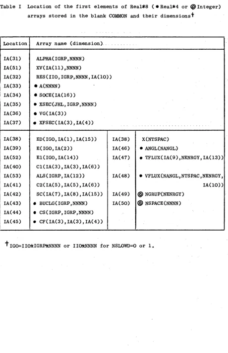
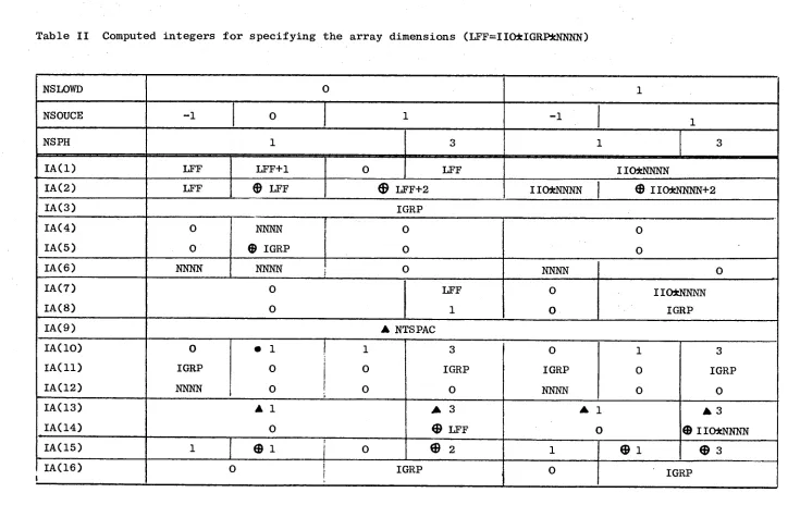
In the MAIN programme, as can be seen from the flow chart shown in the Appen-dix 2, Section 1, sizes of the required arrays are computed based on input parameters and then first-word addresses are calculated for these arrays. The locations of these pointers and the associated arrays with their dummy dimensions are given in Table I which shows also the fact that the storage locations bigger than IA(38) are used in two different ways, once in JNMETD and then again in FLUXCA. The actual values of the integer variables speci-fying the sizes of arrays are summarized in Table II. The first-word addresses and the dimension informations are transferred through a call statement and a part of vector in the blank COMMON is treated as a multi-dimensional array in subprogrammes.

The subroutine JNMETD computes:

(a) The residue 3%*(%") according to equation (6) £" or (17) for a

non-multi-plying system without up-scattering of neutrons ~J and if NSPH=3 ^jJJifyA)

(b) The value of k for a multilayer slab reactor (NSOUCE=0, NSLOWD=0 and NSPH=1) and if L L L > 0 the ratios between Βγ.ι(4)'$ from equations (10) and (6) with S» =0 and Qítf­^í') given by equation (11).

(c) The asymptotic time constant i-<Å\ for obtaining the asymptotic decay constant Σ^{Α"Λ() for a multilayer slab (LLL=0 and NSPH=1) or if NSL0WD=1 the asymptotic decay constant of neutrons belonging to the lowest energy group.

For the problems (b) and (c), the values of Çfa(Î->ï) are first modified ac­ cording to the guess of k .. or 4~ÂA > and for the problem (c) the values of

eff

flf¿*= R*Xi (4n~^£-ƒ) are calculated (see the flow diagram. shown in the

Ap-pendix 2, Section 2). With these values of Çg(£~*j) and (xfi , the matrix

elements for equation (6) or (17) Calso for equations (15) and (16) ~\ are

then calculated by calling the subroutine FCAL (fl^/Ofr ,&, 110, M M . XHíjfÜx

*Μφΐ%%ΦΐΡ/£·<1,

y(*ft?ÍM?*e

that^

}

*=y/(

Z j

^p^) and

£

a

<X,*=ol

which computes the value fàQR*(4r) Jey (flfÅOíj', Λ J d ) f o r η=0Λ/ΜΜ+1 by the use of their explicit expressions shown in the Appendix 1, Section 1 £see for­ mulae (A14)­(A]8) . In the case­where ftjJ+ ft^­f |¿lj < 5 > it calls the subrou­ tine F I Ç A L ^ ^ ^ ^ I I O , JIIj ^ V j P j V t ^ P j ^ ^ V j P ^ f l t ) in which the series expansion shown by the formulae (A23) and (A24) are used for the calculation depending on the values of parameters (XJ¿ (X* and JL (JII stands for the para­ meter range). For computing the first and second derivatives of J»ywith %~\—Ί

and γ=7 > t n e FSCAL calls another subroutine FSCQN. In addition, the FCAL and FSCAL use the subroutine SGMOD (SSI,I,....) in which when I > 0 Xnm,n WÌJOÌÌS i )

is modified to Kj+nt4 n+i £ s e e equation (All) in the Appendix 1J , when

1=0 the summation of (A16) is performed or when K O a multiplication is car-ried out for calculating the derivatives of J«y by using their series expan-sions. The exponential integral EfiOO appeared on the right hand side of

equa-tion (A12) is evaluated by the funcequa-tion subprogramme EP(fl3 X) which comes from

the subprogramme EP(n,x,b,....) in the computer code JN-METD1 (ASAOKA, 1971). At the end of the FCAL, the recurrence relation (A7) given in the Appendix 1

is adopted for computing the functions Jay with q = 2-7 and r = 1-6 (and

their derivatives if NSPH = 3) from the values of Je~and J^with r = 0-7 and

­ 17 ­

After having been obtained the matrix elements, the JNMETD calls, for the

problems (b) and (c), the subroutine PET to evaluate the determinant (10)

C with ­ j s y ^ i j

for the problem (c)

~]

or the corresponding equation for

the problem (c) with NSL0WD=1. The subroutine ITRTON is then used for iter­

ating the process to make the value of the determinant zero until the rela­

tive difference between two successive values of k ._ or /­,¿/ becomes smaller

than EPSK. For the problem (b) with ,LLL>0, after obtained the converged

value of k

, the ratios between the residues are calculated by evaluating

the cofactors of the determinant by the use of the subroutine SOLEQ which

solves a system of simultaneous linear equations.

For the problem (a), in addition to the matrix elements, the first term on

the right hand side of equation (3) fand if NSPH=3, the right hand sides of

equations (15) and (16)J or if NSL0WD=1 the right hand side of equation (17)

fand the expressions corresponding respectively to the right hand sides of

equations (15) and (16)J is evaluated with the help of the subroutine CCALC

CtfJ

* M IIQ,

MMMM,

*fa&4rtyth (Φη^^-Μ

) ■

The

CCALC c o m

P

u t e s

(-t)2Cf^K^j^^)

MMMM+

^^

J

t-4^jft'/)

w i t h mm=1

'°

or

"

1 b

y

usin

e

t h e i r

explicit expressions if

tfj+ofi-l·\¡J[

j^3 or the series expansions otherwise.

As is seen from the expression (A43) it uses the function subprogramme EP

for evaluating E . The residues (and their derivatives, for NSPH=3) are thus

obtain in the JNMETD by calling the SOLEQ to solve equation (6) fand equa­

tions (15) and (16) J if NSL0WD=0 or (17) fand the equations corresponding

respectively to (15) and (16)J if NSL0WD=1.

The subroutine FLUXCA computes for NTFLUX>0 the total flux and/or for

NANGL>0 the angular flux by using the values of the residues (or the ratios

between them) obtained as mentioned above in the JNMETD. As is seen from the

flow diagram. . of the FLUXCA shown in the Appendix 2, Section 3, after having

calculated the angle points (the values of

JUL

) at which the angular fluxes

are to be computed if NANGL>­0, the space points ( 0 < 5 < f ) are determined

in each region and the total fluxes are calculated at these points with the

help of the subroutine GCAL

((X.K

tt.ktt-iì-A

}

ITO,

M M M M ,

^fyffi¿­fa^C^H)­¿ 3

>

(Zfypa

i

-¿

r

f&(

i

Ha5-0-¿'}

)

if NTFLUX>0. The GCAL computes (¿>(Γ}^Ρ,'^­^

ΜΜΜ+

χ

*GA<X*\0(lK2$-ÅjÅjtV)

f o r

MMMM=1, O or­1 f see equations (8) and (17)­(20)3

es

ftjl+l0(j^(2J'­^)­íí I >*5 o r the series expansions otherwise (see the Appendix 1, Section 3 ) . For NANGL>0, the FLUXCA calls the subroutine FMCAL (ocÀç/Jpf-j'yjL

μ, HO,

MMMM,

ZjV-PJ-føia.hs-O-Jil,

(^P&fteífW-iMJ

) which comput

UXTJ^P.^^^Fpía^OC.ijJjJÁjJiJi) with MMMM=1, Oor­l for calculating the second term on the right hand side of equation (7), (13) or (14). The FMCAL uses the series expansions given in the Appendix 1, Section 2, if (0(»L-+

In the case where NSOUCE=l, the FLUXCA evaluates also the contribution of un­ collided source neutrons to the total or/and angular flux according to the first term on the right hand side of equation (8), (19) or (20), with the help of the function EP, or/and equation (7), (13) or (14). If NSPH=3, the above­mentioned calculations are followed by the evaluation of the mean emis­ sion time t and the variance ^­a of the time­dependent flux due to the delta function boundary source. For the angular flux, these are written as follows [see equations (12)­(14)J:

0

which are calculated in the subroutine VAR'IAC.

4. Remarks

Since we have already developed a general formulation of the j„ method for Ν

­ 19

pressions or series expansions obtained under the assumption that the values of all arguments of the function are small. Therefore, in the case where the ratio between the arguments is very: large, it is possible that the function is evaluated with a large rounding error. In such a case,it will be a crucial point for obtaining an accurate result which order of the j approximation should be applied to the calculation, because more complex functions are re­ quired for the higher order approximation. Generally speaking, the j approxi­

O

mation gives a reasonably accurate result for almost all physical problems. It saves also execution time of the computation by about 30% compared to the j calculation.

Typical running time on the IBM­360/65 is nearly 1.5 min. to obtain, in the context of a 7­group j approximation, the total and angular flux of the lowest group neutrons at 3 angle and 6 space points in a 3­region slab with a stationary boundary source. However, the calculation of the time moments of the time­dependent flux requires a rather long time. A 7­group j cal­

D

culation takes about 10 min. to obtain the first three time moments of the 7th group angular flux, resulting from a delta function boundary source, at 3 angle and 6 space points in a 3­region slab. The j approximation requires

«5

nearly 7 min. for solving this problem. All three sample problems shown in the Appendix 3 take only about 10 sec.

It remains to note that, in the present code, the introduction of the lateral buckling (Prf + Bo )« to account for the finite extension of a slab system in two directions leads to modify only the values of C(9­>9/) as if the absorption cross section increases by (&+Β$*}β/(32Ttr$) b u t not the value of Σ-tri

[image:24.595.76.537.68.779.2]

Table I Location of the first elements of Real*8 ( · Real*4 or <§> Integer) arrays stored in the blank COMMON and their dimensions^

Location

IA(31) IA(51) IA(32) | IA(33) IA(34) IA(35) IA(36) IA(37) IA(38) IA(39) IA(52) IA(40) IA(53) IA(41) IA(42) IA(43) IA(44) IA(45)

Array name (dimension)

ALPHA(IGRP,NNNN) XV(IA(11),NNNN) RES(IIO,IGRP,NNNN,IA(IO)) • A(NNNN) • SOCE(IA(16)) • XSEC(JHL,IGRP,NNNN) • V G ( I A ( 3 ) )

• X F S E C ( I A ( 3 ) , I A ( 4 ) )

E D ( I G O , I A ( l ) , I A ( 1 5 ) ) E ( I G O , I A ( 2 ) )

E l ( I G O , I A ( 1 4 ) )

C 1 ( I A ( 3 ) , I A ( 3 ) , I A ( 6 ) ) A L S ( I G R P , I A ( 1 2 ) ) C 2 ( I A ( 5 ) , I A ( 5 ) , I A ( 6 ) ) S C ( I A ( 7 ) , I A ( 8 ) , I A ( 1 5 ) ) • BUCLG(IGRP,NNNN) • CS(IGRP,IGRP,NNNN) • C F ( I A ( 3 ) , I A ( 3 ) , I A ( 4 ) )

I A ( 3 8 ) I A ( 4 6 )

I A ( 4 7 )

I A ( 4 8 )

I A ( 4 9 ) I A ( 5 0 )

X(NTSPAC) • ANGL(NANGL)

• TFLUX(IA(9),NENRGY,IA(13))

• VFLUX(NANGL,NTSPAC,NENRGY, I A ( I O ) ) <§> NGRUP(NENRGY)

(§> NSPACE(NNNN)

Table II Computed integers for specifying the array dimensions (LFF=IIO*IGRP*NNNN) NSLOWD NSOUCE NSPH IA(1) IA(2) IA(3) IA(4) IA(5) IA(6) IA(7) IA(8) IA(9) IA(10) IA(ll) IA(12) IA(13) IA(14) IA(15) IA(16) I 0

­1 0 1

1 LFF

LFF

LFF+1 φ LFF

0

3 LFF φ LFF+2

1

­1 ₁

1 3

IIO*NNNN

IIO*NNNN Φ IIO*NNNN+2 IGRP

0 0 NNNN

NNNN φ IGRP

NNNN 0 0 0 0 0 LFF 1 0 0 NNNN 0 0 0 IIO±NNNN IGRP A NTSPAC 0 IGRP NNNN

. 1 j 1

0 0

0 ' 0 A 1

0

1

_{Φ ι}

_¡

_o

3 IGRP

0 A 3 φ LFF

Φ 2

0 [ IGRP

0 IGRP NNNN 1 0 0 A 1

0 1 0

Φ 1

3 IGRP 0 A 3 Φ IICHcNNNN

φ 3

IGRP I CO

[image:25.842.58.782.52.516.2]

References

ASAOKA T. (1968-1) J. Nucí. Energy, 22, 99.

ASAOKA T. (1968-2) Nucl. Sei. Engng., 34, 122.

ASAOKA T. (1971) JN-METD1, A Fortran-IV Programme for Solving Neutron Transport Problems with Isotropic Scattering in Bare Spheres and Homogeneous Slabs by the j„ Method, Report EUR 4601e.

N

ASAOKA T. and CAGLIOTI E. (1969) Trans. Am. Nucl. S o c , 12, 635.

ASAOKA T. and CAGLIOTI E. (1972) The j Method for Neutron Transport N

Problems in Multilayer Slab Systems and its Application to the Optimization of Moderators in Pulsed Reactors, submitted to J. Nucl. Energy.

HEMBD H. (1970) Nucl. Sci. Engng., 40, 224.

KSCHWENDT H. (1971) Nucl. Sci. Engng., 44, 423.

23

Appendix 1. Analytical Expressions of Functions

Since the general formulae of the functions appeared in the present formula-tion have been developed in a previous paper (ASAOKA and CAGLIOTI, 1972), we show here only the final expressions and then summarize the explicit expres-sions and series expanexpres-sions for the functions in the solution of the j ap-proximation.

1.

Jl.iWiiOdx&ji)

We consider here JLy. (0(;}0iij Å J cL") with fty>ft¿?»O because

The parameter range is divided into five:

(a)

-a

r

a

i

-ji>o

J

(b)

-<X

r

(X

i

-¿<Q

ana - t f j + a W > 0 ,

(c) -^+or¿-

fl

í.<o and ft}-or¿-<¿^o,

(d)

ίΧ|-^-οί<θ a W

tff+tfi­öt^o,

(e) «j+or¿­cl<o.

Since Jo-fíOÍijtti )¿'j Q.*) for the parameter range (d) or (e) is equal to

(-tf Jfoy ((Xiι(Χί M' ~èS) f o r t h e r a nge (b) or (a), we show only the general expressions for the range (a), (b) and (c):

*

Yunt-fijjXhai-i-tf+iyunWjrnja')!,

­for ( α )

;

X ^ Í X j * ( ^ , ­ f f

¡ r

¿ ) + H Í X

i f t

( ^ ^ ^

-IrrtYun&jM.ti-wyirHtWjrKijJiilj

i o r ( b ) ^

(Al)

|[X4«(-fljrff¿/J)+ H ƒ XinC-flJiflTi W )+ H#Xi*(-fyflr¿, AÍ )+

- H > * ì i « ( ^ * o ¿ ) - ( - « * >

^ - φ " * < Λ ) J,

íor Cc),

CA3)

where

(A4)

» 7 <A 5>

Ν/ -ƒ ^ (Of+iX'+J.'ï1*

lun

^&><ί)=ψϊ?

ί

ψ*Η4£

0

(¿4)L+¿A)l

^ ^ ^ £ / ¿ ) = Y / ^ C ^ ^ ^ ) - X j f i C - « / , - A í W ) .

CA6)

The functions which we have to evaluate in the j approximation (which re­

quires Je γ S with q=0,1,...,7 and r=0,l,...,7) are J0y and J^ywith r=0,l,...,7, and J»Q and J·» with q=2,3,...,7, because, due to the recurrence formula of the spherical Bessel function, we have the following relation:

The explicit expressions for the Yyterin of these functions, £ ( 0 (fj/^j/ ^JjY(ftjy^£/­4víí)S;are written as follows f see equations (A1)­(A3)J :

V' *

-

25

-fc

Á

l

*' -4Í C M ) ! éj,

c

" CWOH ( 1 ^ ! * · * * ' *

V*¿**I* + >,

(AIO)

for r=7 (All)

The expression on the right hand side of equation (A8) leads

^^|j4/ir^x^(^^)=

^Xi(z)-e

x

+z

a

E

4

(-z^

.

y=o,

( X ^ « - 4 X ; ( i ) ] / + i i - ^ . x ) ^ ^ w )

;

r=0

[Χ^χ)-^χ^α)+^χ

3

α)-^

3

λ4(χ)+^Χ5^)]^4.

t(<

-JO

x+

45

lXi«)-|

I

Xatt)+4|

k

X

9

«)-^)C

f

aH^Ätt)-^X

4

(ö3€

ac

+

c ■ *

W«>-áfXa«H|^x

a

w-^iX

f

w+^x

5

(x)-^X

í

«)+

+_33_ γ

η Λ ί Λ / Ί - Χ - Μ - - ^

r»-¿LT3

+

M ^12.^5·+

+¿H

¿

X

e

) *

a

£<(-*>,

r=6,

[ X

Y

( x ) - | ^ X

j î

( x ) + ^ X

3

C z ) - ^ X

f

f z ) + | ^ X

5

c x ) - ^ r

s

X

6

( X ) t

+

^ ^ « " ^ Λ

α )

Ι

Λ

^ Α

χ +

^

χ Ι

^

Λ

(Α12)

+ ML·

y f - . i l r

5

+ ^ î , x

é

- ^ > 7 X

7

)X

a

E/-X),

y= 7,

where Χ^ΟΟ­ΧΧ,*,«)­*«!, W>=M Γογ X«(X)rJ¡C«*HO!Χ ^3 a*i Χ­flfWMÌ. The XJ­Μ,Ι term on the right hand side of equation (AIO), ­flffi % (~Λ*Α\ (Y-AV *

* X H S H C ° í ' f r i ' f l O ' r = 0~7' c a n e a s i ly b e written down by replacing Χ^,(Χ)

in equation (A12) and % * * in the coefficient of %*%&) by ­X*rø OO/f («+­2)0$ 3 and ­3C^(«H*5Äp , respectively. In the same manner, (~tftfjOfc Í ('JY }\{f-¿\?

* ΧΜΛ n(0(¡,tí¿Jcl') of equation (All).for n=2­7 can be obtained from the

last equation of (A12) by replacing repeatedly Χ« (Χ) and X in the expression for Χ^4ί,η ^ ~X*H&ViU&X)CCI and -Χ*/ί(4»«)θζ[ 3 , respectively, to get that for Xi-MH^fl+4 f compare (All) with (A28) J „:

The extra terms consisting of ^ ^ o r Ύχ^γι on the right hand side of equations (A1)-(A3) give the following expression:

+

N)^Yii

A

(-^^¿;oi)+H)

r+í

Yí^C-^-ar¿,úl)l = 0^ -for all cases.

(A13)

l=o, 1=2,

­

27

For q=l­7 and r=0, the expressions are the same as those for r=l­7 and q=0

shown in equation (A14) except for interchanging OC.· with 0f¿ (and vice versa). The expressions for q=l and r=l­7 are obtained by taking respectively the

sum of those for q=0 and r=l­7 and the following formulae for q=l and r=l­7:

Similarly to equation ( A l l ) , the expressions for q=2-7 and r=7 can be

writ-ten as

a

Expression for

f

| , 7 > £ cjgjgsg,

IM>, ,

t*ie)

in which ( 0 , 7 ) 4

i s t h e e x

P

r e s s i

° n for (0,7) given by the l a s t equation of (A14),

(1,7) stands for the l a s t formula of (A15) and (n,7) for n=2-7 are

+ ypo(?+100101,

rtígc<^/-|¿c^^^

29

-- nio (ocj+jL?tf+ ίψα?+ *ψΖ(ψ<ΐ)

2

+Χψϊφm39S5o

i+5ioa

ií

+

+45í7¿oar¿

4

+57"5350Oaf-f

31213100 }

}

«fri» ^'

Í2

^-

m

^-

2J

&

22

-

m

^ -^ m+M»¡-«

+

¿>

«^Ί,η^-Μο-®^-'^^

+1ψ£

(

^{ίψ5^

+

éooh^mnVOO(i

4

i-72037350oa

i:i

^ni72.4?êO-^0(

iH

}

.

The extra terms on the right hand side of equation (A3), 0(\0(:Σ Η ) Σ

~(-Ό* ¡24ifi{~^i~ML )d-*)~l are always equal to zero except for the cases where they give the following expressions:

-fdod/^, P4,r=0;

- -f «i

{orf*itf-3d-2yo(f, tø r=0;

4<*d í3tf-5Q(?-5d?-Jio V (tf, \*3, Y=0,

aifrctf-ioyW+loftesd^ofâ

- Odd O5af-j0tíftí

í

*+24O(Xtt'-l00<fd

J

+L3

(

f+

\ή20(Χ*+\5\2 y (tf,

î=5, Y=0,

- (ψ*?- M50fat+V§mt)t- 35<xfr2W(Xfô-23W?-iï55d*+

Hi30cf-23W(Xftd*+lSÍO(¡-2moíi-nUd-moJ/o(f

}

£=é,Y=0,

αιΙ{ψ{-ψο<*φψο(ΐΦ^

-í^^

4

-^K^+^^

4

)¿

a

-3í5^+23/O^

a

-3OO3«^-30o3A

(AIS)

In t h e case where Ctt+ufi+lcU i s s m a l l , we can o b t a i n t h e following s e r i e s

- 31

+

<rtfY

3Á

tobrKi,ly*\-&Yu

<*}>M)+

<rrf

+i

Y*A <r*¡r*c,m

­

-ΜΫΥ+ί-η,^ΛίΜ-ί-^

­W^^^(­^,flf

i /

flt)(­fl}+flf

(

+

í

l)*t

where

À<

($W)l{r+À-/rï)!

Y

«Xì,o(; d")- (er+fif+jJ+

2

7*

LÍÍñ2üIt£^2i

í

(A20)

^ ^ / / f l r i ^ ) = Z ( ­ j ) ~ ^ , Y

w

(ef,flr£„0,

CA21)

Y

5

«^«U)= Ζ (47«asÕ| YtfCtyO^);,

(A22)

and y is the Euler­Mascheroni constant. For the parameter range (b),

(tfi'tOCi+d ") ö_> the argument of a logarithmic function multiplied by

ΥΛ. (Mi/ Od j d ) and the variable of a series expansion multiplied by Y¡mWfO(i¡d')

on the right hand side of equation (A19) are replaced by —(uC;+OÍ¿+d^>^ · ^o r the range (c), in addition to these replacements, two (ofj—OifidYs > *ke ar­ gument of a logarithmic function and the variable of a series expansion, are replaced by ­(GU­tfi+tfO S .

u- fV-fø. iloita f Jk

c­

i«F*&l

>) +φξ

{

*ì ' ^ f** (-Wf*^

»

f

Ì_(v ufi? i £ w f ( W ^ X - « j - ^ t l ) I

fen

γ

=

Λ

3*W

3

De+a¡l?*¿$t

ΛοΤϊ+π·

¿ti?) at Λ oft r

oft\3

f

gp

f

S ? ;

+

# i a ? W «

* ar Jot?

+

?tf£*J

x

ΐ=0,Υ=3,

^Γ4ΐ,.

0

ο^ -fifi

4

./.»

„ . S í f ^ ^ i í i

+

f.l.

t

S.âJÎ-l£îi

4

3.ûif

+

x ^ - 3 5 Ä L

+

¿ 3 £ T S J £ ƒ35 4o5o£WÍ

+

2Í.iÍlx

X

M4^)(­4^Í

Λ «¡

W^Mlώ^φ^φί, WIS,

33

AH agi^N g re

d[

7 /■ r(g$ioii4^£^±o^ -r,

oa [ L

v

Ug

+

U

TW'W

* ftcO^il(4j-¿42)(-a]V+¿)

* *r ** net?

¿rm ffl3C<i

2

.M51X* Μ3#£ (1313 5225a2\iM#¿)d*

+

(Ma_

a^Wo 6o W^TW

"Top

\ ¿ο 3ΓΦ

ί

or+Jc(r

[

*F

Kr j

í . i i

2

u l á l í

[(Μ#άα2ί#ίιΧά£>

71

2(tdfJ(*

i

*Kiïh(-*j+*L+d)·,

XM

U4-0¡ldX-%

+

¿+d) 1 ' *<>'*

cji ¿

+

t ^

tofr

+

V3

Ύ7&)Ή τα?*

+

αΐ\

4

ofc 3K?)

IjlT 7 3p

+

é ft? 13 3

cfc)oí*+6 al· ^ olí

1

* *o<? +W

[

* 2Wtr

d<ym3o£

Mg¿

x

ío5oc¿.(£L 23*5κ*2ΗΑο£\£ (¿s

mo£\£,

Ύ^π

+

-2ΐο^'Ψ^

+

^^

+

\ψΐ2Τφ*^ΤοΓ*)ο(?"Ur-tf α? V

4

0(ii-jL±mü£

4?Π tf > 2531/¿

^«L

?

^riL-517^

+

£25jÄjl_€223flS

x

•^ί

Èõ+2fo%*-wÍfr+W&-ltot*(™

Χ«?

60

W

MljfJ*

^Õf~ÍSo 72 ^

+

>?0 ft?/ft? W5

120 0!?)W

4røfti*i

+

^p

X

35

-iWaí±22BÍ«í

iAf^iÆaf,

7/?af

4

55JS?af

é

>> ¿

4

(M i

+

w í

a +

w ^ ^ f t \

é +

Í 3 F r

+

^ õ f t ? / ã ?

3no^°yo^

ì

^

-2 3?

3 «i* Í _ u ¿ 35 ft¿ ,2íáAí? j?3^

AÍ·»

, ¿go/ ftî'a ι r 3 . ¿5£fr? ,

* itä Off 3οο3 Ofi

io

\d

3

,

(35

, 35

Off ΜθΦ

Λ

23JQ(¿,

3P?3Ê£

\ dl·

\3f4

+

ί^

+

ί#α?

+

7^^^

+

\5«

+

:ι##» 1 « ^ apriste

4

+

ilft¿SÜ

04

JL_if i tf^Mi¿2í^í^iá2l £=4 r=7

4

SS ft·-/

1

A¿<°

4

/53é

ί ^ ΐ φ ρ ^ J

J

*~^

r

h

°<*C3 5

o£ m ftj

4

i£La¿£

3 1 . « £

+

^ Λ ± ί °

ääQ(£

.(Χ,+ΑΙ&Α.

õflss Sfap-äsö^F-ftb^ w ^

+

3 ^ ^ - H " ^

+

w

+

3 ^ ä ?

+

f2i

, ¿ I g g ι 75 ftf* , 35 ft

1

,·

6

, ?J5 ft/ ,

¿93 Oft

4

*

3θθ3θή

42

\ d*

.(Í3..+

4

ifê<

4

A)^^

4

^ft^ft^

4

lW

4

wÆ/ft7*

mw+}

x

™l (¿^^(-¿¡WM)*>

^d^o*m^iipo^^wo^^mo^

+

ù2iow> 3WX?

2

w*w

,St3i o¿,m_oc¿JJ]i

off, ^301 off

, 3533 ff*S

d\(UÆÆ2Xtf

x

37

\Wo wfforri2foo(fJa-i \W> ftoött'<x¿° moixp-ï 115&¡i*

^

l

(­sWix^rfj)i ν ι

Í3

4

75^

4

^ M U

ά

Γθ(ί

φ(-«

Γ

κ+ύ r

,Oftd<

33 af ftf J l Ai

4

2¿L«íí ^5. «if üLftii? ^ ft/

3

,

42l off*

,

+

ÛJ­7

r wpf im off ion ofr ~ nv*t W ~ ^ixf

/«* 3?""

Tmw

x

v&ofp

i ^77 , g ftjf , J75

tf, 115 Off.

3/5 flf ,

23\

ft¿° , ¿goffi? Ν ¿ / ^ 2

+

4

V 7 f ø

4

5 f r a ?

4

w ^

4

W a ^

χ3ηθ£.245θ£_

χ

345 fri', ¿f3 ¿if,

3 0 0 3 < ° ^

4

, ^ . V g 5 f t í

a

. 3 f 5 a f

f l

*1θΛίφ

+

512ψ + 5&ψ

4

/ ^ ^

4

W ^

0

/ ^

4

\ 7 õ 5 ?

4

ã 5 ? ^

3 4

« 5 « ?

+

+ i É 5 ^+

4 2 i a í í i i í táS.

,3j5 0ff

+

3?5 0ff 715. offsjf

(J3_

*M

<ΧΓΐ024ψ)(xr\3o12+TmK

Í

l+

imW^3oT2^Jßff

+

\lo2f

+

,Jä-Qls1\

Off\d

i0

(234 ,2j_</f^dí

2

4i ¿«In

ffo+afr¿X­tt­ft+¿)7

^512 ar 1024 al· )W m& ionWfJoip*5120

Οί^ίΜ^φ

(-¿.^φh

<£< dtèl+izLítxâsL °ú?4.2M.9¿ (2pm. WH off

, ¿woj*, ggggg.gi.Sv

apCiõu^ionW'¿Wow îffîfow

^¿mõ

'30720cfrmõψ

+

2Wfo¡χ*)*

y<t* ,(34113 ,32m off''MolapAJ? (31451 mi Off. 10251 rfu'

*(xf\imo^3ëmoff 30720of+Jotil· \M*o Wfô af 102400 ofria?

4

+

MM

+

Í2222£íf.if

(άΜ

+

2 ] 2 Σ ^ ^ ^

+

ΐ4η^_α3Α^-ι,

+

¡(ff f 421 33_tíf 2j_tf

ã-Of£

25 Off

■

(421

,

231 off

■

Jrø

<*,

i^llÎm~2oit^-4o%W~2oi^~1(>3Hc(

i

^

\2¡F$*2<nXCff2oTtal·

,m of¿\j£ (iooj

,

613 a£,45]5tf, Í2250¿\J+ , (ml±åiP50ff

,

■

135 Off \¿

(2H5

i

m5jf

i

\2mtf-sd*(ÅQQi,]å3-0ff\d

i0

(213

,

where Tja< > b J stands for the fact that the expression is the same as shown just before except for interchanging a with b (and vice versa). In addition, the expressions for q=l­7 and r=0 are respectively the same as those for q=0 and r=l­7 except for interchanging Of/ with 0f¿ .

The coefficient of the series expansion on the right hand side of (A19),

Ysm^i'Ofijdy (.Ofj+Ofi+d) , is written as follows (by the use of abbre­ v i a t i o n X-Ofj+Ofi+d ) :

WÕ\ ?

Tff-Oj

2 2 Τ β_η ν i

WfttO!

(<mx)\ Ob >

*~

v

' '"^

X

4

_ i

IL

%=0,Y=2,

m m m+2·)

¡ or¿ cm+3) ι

ofâ >

-2—

­_¿L_ JL + _30_

X* 30_ X¿

ï

= ö

v

=

3

(«ΦΙ

(m+2-)ÌCK

L +

(W+3)!Oc

a

WH)!a¿

3

>

* ' ■

>

(îTîtO! ( » 2 ) ! β ί+( « + 3 ) ! ^ (WH>! ft¿3 tørøi 0 ? , r υ

CffHOi

(«Ι+Λ!

a¿ fw-3)'.^

cimi! afm5)iofl·

muy.apj

B

2

42

X ,420 X* 2520 X

3

,

9450 X* 20ll0

j £

.2oll0 ¿

w+oC m+2)i ofc ^(mrtV. off ctn+inã? (m+sv.af

cw+¿)( a¿

5

<m*v\ off;

_2

Sí

X

, 75¿

X* Í30O X

3

. 3­f¿50

X* 424740 X

s

■

(«WÍ! (W2)ÍOÍÍ

(w+35!a;·

3

õwiJíârt

8

(«f5?!fl^

cm+oiar

270210 X<> 210270 Χ

η

t=0,Y=7

(A24)

39 ­

(A25)

2.

F,íofiA>fjMj¿)(í)

We have obtained the following general expressions for three different para­ meter ranges £ β st Ofi (­2Jf~­J )­fll J ·

(a) /3­or¡>o;

rZftøiftp-wfZfl'crif,/.·), μ>0,

(b)

p-0fi<0

and p+tf¿>O;

(c)

|3+íX¿<0;

4

*

i F f

\-%<ίΧι,ρ,ρΗ'ΰΖι{-*ιφρ, J**

0

'

4KiYM.

. V — - - —

- «'«

CA26)

(A27)

where

(A28)

Tp(^/()=(¿/|

o

í-o

r

(f)

'-feõírepST'""·

<A29)

The explicit expressions for J?p(Q(,ß,U')yfrft0Hß)ßA.] with ρ = 0­7 are as fol­

i {W%*31t{%¿4

3^f#)%473^5(^^370(^^35ffA

+^35(&)

7

J, f=7.

(A30)

The expressions for T» (OfjBjM·) with p=0-7 are

CA31)

,3

41

-In the case where the value (θί+\β]}/\Μ\ is small,

Ζγ(<Χ,ρ,ρ4ΐ

?

(ο(,^ρ=

+1-10(ífH°s$? J (-"fi?,

Mj

(A32)

The series expansions for the expressions (A25) and (A27) can be obtained

by regarding the formula (A32) as the series expansion for the function

3. GF(C(Í)O(ÍJ~5;Á;¿')

From the expression for pi (OfijOfi, %,M,J'jJii shown in the Section 2, we get

(a)

(3-(Xc>0;

*X¿C

r

(Ofi,Ofy$

/

J-

J

d>'Up(0fL,p-HÍ'U

f

(-Ofi,p

j

(A33)

(b)

p-a

L

<o

arid

(3+cfc^û,

WiG

f

= Up-(cfL,pw-47Up(0fii-p

+

Vf

(#£,p,

<

A 3 4

>

(C)

pO(

L

<0;

W¿G

f

=H7U

r

Wi-p-Uf l-ti-p,

CA35)

where

U

f

C^p>

t

0^4

w

ff^,

(

^tgV^-^'H^

p

n

Χί-^Ρ+ΠοίψΤ^Έ,Μψί,

_(A36)

ν ω

e^-tdfU

aamu

'f__täH^___

Vf 'P' £ 1

1

'

0ï

)!i

(Ä)

r-ir -<£ o¿+f-#

f

/¿])¡«rpAHr-ijtO ·

(A37)

The explicit expressions for IJ» (#,0) and ^>(#/ß) , p=0-7, are as follows:

43

-U

t

=-[|(^-f(#r

+

f|(#/x<-#)-o-^l(#A^?^-^^ár-CA38)

VoW,p,=2j

Η»π-ι°°Φ)&-ψΐ

<

Α39)

For small values of #+1/31 , we can obtain the following series expansions for Up C tf, β ) with p=0-7:

" '%

Hr

dfm\

^

(wairí-iWHO^fêfW

3

-

(50-405%-^5(H4^f42i{êY)(4-hl(^p

m

í

^U^^-^mm^i^ (w%y*?-

45

+f725

$f )<rf+ (3Η-ίοΐ£-5ϊϊθ{£?Η130

(fefr WO (£fr

W(&ft«l--

§T{W5-n50(&f44o315

(fej

1

) (<-&)]

V+pf?

-3W(£fj11l

S

~(245-1l0%-W0(£fa

-42loo(§)\47325 ($f)<m?+

m-3mjr-3o24o{§f4W5o(&f45im(&f--

¿2?7θ(#/)0

ΐ -

[225^ol1^-2{35l{^

r

\o14^442m5[^442414o

(M--4W5fëf)flL-315[5-Jta@fa

(A40)

The series expansion for the expression (A34) can easily be obtained from (A40) by regarding "\/„ (#,0)= 0 f o r a 1 1 P«

4.

Cupial é±É2

S i n c e

Cu.te¿,rj¿,cr

4

>

H/Pp^dji/iY^a^^ fo,

the use of the expression for J­l gives the following from (B=Ofj¡-d~) '·

(a)

a

r

of^>¿j

^^j/^^'^0=W

?

(«¡­,(3)­H^Wj(­^P^

(A41)

<

b

> ^+ftj>ít>ft'

r

^·;

(Χ^0μ = ^(^·./3)+5^(^)3),

CA42)

(c)

d>0(i40fj,

#¡^$¿-0;

where

StoBÏ-litâfïtf

tat­ar­Oí!

ψ

4

,

ß

fl

(Α44)

The expression j? IVy (06ß)/( 0 is the same as that shown in (A12) with

X-~(0f-+ß') and 0(¿:z­p( . The explicit expressions for $t(&S0) with q=0­7 are

- 47

4

fKHw-lí^)

í

íw)J}(-^p^

*=

5

,

^(^Ì^>^4)%mì}

Π«Φ f,

(A46)

where f

Ä

(fl)s­f

(fl)+efl!/(fl*»t).'

W

"f

4

tølXfl+iVrøH).' .

Appendix 2. Flow Diagrams of Computer Programmes

1. MAIN

( START y READ title and input integers (see § 3.1)

I

(

ν

No

J

>

\

l The first integer >· 0 J >l STOP J

Yes

WRITE problem classification and title

Clear COMMON

Dimension assignment for arrays (see Table II)

Ì

Calculation of storage locations of arrays (see Table I)

WRITE required storage

I Requi red storage^available storage

I

Yes

J

No

CALL JNMETD

i

J

LLL

> 0 J

Κ

Νθ

( LLL>

READ all input data left for the present problem

Clear a part of COMMON for the flux calculations

CALL FLUXCA

49 ­

2. JNMETD

Γ ENTER J ^ Γ NSOUCE > O J

No

Yes

■^\ WRITE problem classification

READ & WRITE SOCE READ CK1, CK2, EPSK

READ VG, A, BUCLG, XSEC

( NSOUCE = 0 J Yes READ XFSEC No

2't=B/

/

(3Zt

r

­)+Zt ,

ALPHA

=Ztr*A

( NSPH = 3 V Yes

No

­5»j xv = 2 t r U Λ

NSOUCE <

ZJ

Xes ALS = ALPHA

No

£ S * U + p = ^ * ( i ­ » p / 2 t i *

*

Yes

^* ■■ ι . ^ γ rtg ■■■" '■■■

( NSOUCE = Q ) Ζ] g T j ( ¿ ­ » j > X¿(V%)¿yXtc

No

WRITE A, C S ; J P I = 1

C

NSOUCE >

U

No ^ CK = CK1 Yes

( N S O U C E = O ­ ) &\ NSLOWD > O )

( I I I I > O

J^

Yes

Yes

READ & WRITE RES

No

Cl = CS+CF/CKl, WRITE CF

Yes

J P I = IGRP

i = j = I G R P

No

ALPHA^ALSiM^/Vi + C l ^ U M ) ) ,

cha^p=cs^¡V(4-^v^c¡V(^M^

Ο­

^ NSLOWD = 1

Ι

>

Yes

J = M = JPI

No

Matrix elements E = (XfrOCj ( J - * M ) X ["see e q u a t i o n s ( 3 ) , (15) - ( 1 7 ) ] ,

ED = ( 2 & - M ) ^ ( ^ - )M K HJ j r , m = l^NSPH

or ΙΛ/NSPH-I, by c a l l i n g FCAL

( NSOUCE > Q V

Yes " ^ Next page ED = E

I

E = C2 * E/Cl

ι

—

DELTA = det | ED | by calling DET ["see equation (10) }

WRITE CK, DELTA C2 = CS + CF/CK2

JK

CALL ITRTON

Further iteration

Yes

Converged

WRITE CK

(

LLL>0 V

W NSOUCE = O }

Not

converged No

©

RETURN

Yes

RES = cofactor of the matrix E by calling SOLEQ

WRITE & PUNCH RES

51

-^\ NSPH = 3 ) Yes

ι

No

¿ζ

KK = 1

c

E l = E

NSLOWD = 1

C

}

Yes

J = J P I No

S O C E j > 0 Yes

No

so = o

so ­ W O S j K j P / ^ f

C

%ir

by calling CCALC

EJJJ.

= right hand side of equation like (15), (16) or (17)

by adding SO term and summing up over energy­groups

CALL SOLEQ for obtaining (­gj­) ­fJ(T, Λ )

at

A=Z\

k

V\

by solving

( £ ) *

( ^ ' U ) =

( E L F )

i

Γ NSLOWD > O y Yes

C

No

NSPH =

3)

No

The last term on the right hand

side of equation like (17)

Yes

■$■ o r / a n d ·4Ί*$ t e r m s on RHS of e q u a t i o n s ( 1 5 ) & ( 1 6 )

WRITE & PUNCH

jck-4

a t A=2i%

Yes

< KK = K K + 1 < NSPH

3

No

f77 j< Y e S f J P I = J P I + 1 < IGRP J < ( NSLOWD>0 j

No ψ

γ

No

3. FLUXCA

Γ ENTER V

READ NGRUP, NSPACE

NNNN

X NS PACE < NTS PAC

k = 1 K

No

WRITE Σ NS PACE _K

Yes

( NANGL > O ƒ Yes No

K = 1

Angle points ANGL

RETURN

ψ TYes ( NSPACEK>0 J >^K = K + l ^ NNNN. fjfc

)

Yes

Space points X

WRITE Κ,Χ

If NANGL>O, WRITE ANGL

J =1

Yes No

J = NGRUP

\ f Yes WRITE J

> '

J

^( J = J+l

S.

IGRP )

53

-i

KK = 1

No

( NTFLUX> 0 Ì

jYes

^ Ρ \<0") Go by c a l l i n g GCAL, c a l c u l a t i o n of Q ­terms on RHS of e q u a t i o n ( s ) (18) f, (19) and ( 2 0 ) ]

$\ NANGL>0 y No

Yes

I

Yes

­$»i KK = KK+1<NSPH )

R 0 p = ( ^ ­ ) Fp by c a l l i n g FMCAL, c a l c u l a t i o n of Fl ­terms on RHS of e q u a t i o n ( s ) (12) f, (13) and ( 1 4 ) 3

Yes

­^ SOCEj=Q. QR NSOUCE < O | No

No

)

If NTFLUX>0, the calculation of the source term on RHS of equation(s) (18) f, (19) and (20)]

IF NANGL>0, the calculation of the source term on RHS of equation(s) (12) X, (13) and (14)]

If NANGL>0, WRITE X, CALL VARIAC and WRITE the values of equation(s) (12) f, (21) and (22)]

T i t l e

L J_

keff euess

Χ

1st slab 2nd slab

5

1.1

I.

f ·

5

Å

• 1

[.8

Γ

• 1

• 8

TFST CASF 1

1 . 2

1 . 1 . 2 0 _L 4 0 _L 6 0

__L

80

_ J

1-GRCUP (IIII=C,NSOUCE=C,NSLOWD=0) 1 3 A 4 1 2 1 14 1 1 έ 3

. 0 0 0 0 1

1 . o 9 . 9

l>

ö c CD Β α ω α c r+ α C+ Ρ l-b ο 4 CD CD U I

1st group flux at

6 space points

T "

2 0 _{4 0 6 0 8 0}

2 . CALCULATION OF THE FUNDAMENTAL OFCAY CONSTANT CF A 1-REC-ION POLYETHYLENE SLAB

T i t l e

Guess 4-Jbk

V e l o c i t y T h i c k n e s s B u c k l i n g

BY THF USE OF A 7-GROUP MODEL AND THE j APPROXIMATION

7

L J _

20

_ J L i _{_ L _} 40 _L _{_ L _} 60

TEST CASE 2

. 0 0 0 0 3 8

2 8 5 .

7 .

. 0 3

1 J

. 0 0 0 0 3 9 1 7 1 . 2

. 0 4 8

POLYETHYLENE 7 3 A 9 1

. 0 0 0 0 0 1 8 2 . 2 4

( 7 = G R 0 U P , I I Ï I = 0 t N S 0 U C E = ­ l , N S L O W D = l } 1 1 3

1 8 . 4 5 2 . 1 1 8 . 2 4 0 2 . 0 2 4 4 8 4

Cross s e c t i o n

. 3 1 3 4 0 6 . 6 5 9 0 0 1 . 0 0 0 3 1 2 2 2 . 8 6 5 2 9 6 4

.0024435 .916863

[ . 0 2 4 0 4 3 3 . 1 6 5 8 5

1

« 048 .026 .015 .007 .007 .0970411 .0910411 ­=.0425304

.154504 .154504 ­.0423623.104429 .313406 .0641604 .177199 .659001 .2904332 .241389

. 8 6 5 2 9 6 4 . 6 0 0 5 4 9 8 . 3 6 7 0 0 2 5 . 0 0 7 8 5 6 6 . 0 0 0 3 6 6 . 9 1 6 8 8 3 . 6 0 5 9 5 6 7 . 2 6 2 6 0 9 7 . 0 0 1 5 6 5 3

3 . 1 6 5 8 5 3 . 1 4 1 8 C 7 . 3 1 0 4 8 2 8 5 . 0 0 1 8 2 4 7

1 1 Γ

• 0 3 1 94 87

. 0 1 9 3 0 1 3 . 0 0 3 1 9 4 8

Τ

2 0 4 0

( U S I N G THF PREVIOUSLY OBTAINED CARDS FOR THE R E S I D U E S )

T i t l e

Source V e l o c i t y T h i c k n e s s B u c k l i n g

L _L

20

_J_

X

40

_ L _

60

_ L

8 0 Τ

TFST CASF 3 5 1 1 1

VsATER ( 7 = G R 0 U P , I I I I = l , N S 0 U C F = l,NSL0VsC = l , N S P E = 3 )

. 1 0 7 5 7 2 Ô 5 . 4 . . 0 0 9

7 3 . 3 6 2 7 8 1 7 1 . 2

. 0 1 2

4 9 3 • 5 0 4 0 3 8 2 . 2 4

1 1 57 . 0 2 5 5 9 1 8 . 4 5

. 0 1 8

1 6 3 . 0 0 0 0 3 2 . 1 1 6

. 0 1 9

. 2 4 0 2

. 0 1 9

• 0244&4

. 0 2 1

Cross section

R e s i d u e s

. 0 1 6

' . 0 0 1 3 3 7 2 1 . 0 6 4 5 7 8 6 6 . 08457866™. 0305552

. 1 2 7 7 5 0 1 . 1 2 7 7 5 0 1 ­ . 0 3 7 7 5 6 2 . 0 8 4 3 7 8 0 3

. 2 7 6 6 6 9 4 . 2 7 6 6 6 9 4 . 0 6 9 7 0 7 5 6 . 1 4 9 0 4 2 3 3 . 0 2 6 7 4 4 2 1

. 5 1 9 7 5 1 6 6 . 5 1 9 7 5 1 6 6 . 2 1 3 5 0 7 5 6 . 2 0 0 3 8 4 8 9 . 0 1 6 1 5 7 6

. 0 0 2 6 7 4 4 2

. 0 0 0 2 6 1 3 7 . 7 0 0 9 6 0 0 2 . 7 0 0 9 6 0 0 2 . 4 8 0 7 0 8 8 9 . 3 0 4 9 33 7 6 . 0 0 6 5 7 6 9 2 . 0 0 0 3 0 6 4 2

. 0 0 2 0 4 5 5 1 . 7 4 5 6 1 8 6 2 . 7 4 ^ 6 1 8 6 2 . 4 8 5 4 4 6 8 9 . 2 1 8 4 6 2 2 2 . 0 0 1 3 1 0 3 2

. 0 1 9 4 7

2 . 1 1 5 9 9

2 . 1 1 5 9 9

2 . 0 9 6 5 2

. 2 5 8 3 2 6 2 2 . 0 0 1 5 2 7 5 4

­ 0 . 109092G1D=01 0 . 4 5 6 9 5 8 0 1 D ­ 0 2 0 . 12926113D=02<=0o 3 9 4 3 6 3 6 1 D ­ 0 3 ­ 0 . 1 8 5 0 5 2 0 5 0 ­ 0 3

0 . 6 8 9 0 4 4 4 6 D ­ 0 4

0 . I2910933D­Ö3 0 . 8 3 1 0 6 1 5 7 D ­ 0 4

0 . 3 7 6 6 4 9 8 8 0 = 0 4 ­ 0 . 1 5 2 3 8 1 5 1 D ­ 0 4 ­ 0 . 6 3 3 9 7 1 7 2 D ­ 0 5

0 . 3 5 4 3 4 3 8 7 D ­ 0 5

­ 0 . 2 8 4 2 1 0 4 3 D ­ 0 5 ­ 0 « 369 6 9 0 2 3 D ­ 0 5 ­ 0 . 3 9 0 3 2 2 5 4 0 ­ 0 6 0 . 5 5 9 9 202 9 D­ 0 7 ­ 0 . 26603924D­08

■=0.51706} 900=08

­ 0 · 16677956D­01 0 . 1 3 0 5 9 4 2 2 D ­ 0 1

0 . 4 3 5 1 5 9 4 2 D ­ 0 2 ­ 0 . 1 6 Q 7 4 6 0 8 D ­ Û 2 ­ 0 . 6 8 4 8 1 5 6 4 0 ­ 0 3

0.372O8512D­O3

Ol Oi