When A Factor Is Measured with Error: The Role of Conditional Heteroskedasticity in Identifying and Estimating Linear Factor Models

(1)

Munich Personal RePEc Archive

When A Factor Is Measured with Error:

The Role of Conditional

Heteroskedasticity in Identifying and

Estimating Linear Factor Models

Prono, Todd

Commodity Futures Trading Commission

19 September 2011

(2)

When A Factor Is Measured with Error: The Role of Conditional

Heteroskedasticity in Identifying and Estimating Linear Factor

Models

1

Todd Prono

2

Commodity Futures Trading Commission

September 2011

Abstract

A new method is proposed for estimating linear triangular models, where identi…ca-tion results from the structural errors following a bivariate and diagonal GARCH(1,1) process. The associated estimator is a GMM estimator shown to have the usual pT

-asymptotics. A Monte Carlo study of the estimator is provided as is an empirical application of estimating market betas from the CAPM. These market beta estimates are found to be statistically distinct from their OLS counterparts and to display ex-panded cross-sectional variation, the latter feature o¤ering promise for their ability to provide improved pricing of cross-sectional expected returns.

JEL Codes: C3, C13, C32. Keywords: Measurement error, triangular models, factor models, heteroskedasticity, identi…cation, many moments, GMM.

1_{I owe gratitude to Robin Lumsdaine, Arthur Lewbel, David Rei¤en, and seminar participants at}

Bing-hamton University for helpful comments and discussions.

2_{Corresponding Author: Todd Prono, Commodity Futures Trading Commission, O¢ce of the Chief Economist, 1155 21st,}

(3)

1. Introduction

This paper presents a new method for estimating linear triangular models where

mea-surement error or endogeneity e¤ects one of the regressors. Examples of these types of

models include (i) asset return factor models where one of the factors is either measured

inaccurately or an imperfect proxy for the true, latent, factor or (ii) restricted VAR models

from the empirical macro literature. The traditional approach to identifying these models

is through the use of exclusionary restrictions on parameters a¤ecting the conditional mean

or, equivalently, through the assumed existence of valid instruments. In contrast, this

pa-per demonstrates how a certain parametric speci…cation of the conditional heteroskedasticty

(CH) a¤ecting the structural errors to the triangular system allows for identi…cation in the

absence of traditional instruments. As such, this paper contributes to the literature on

iden-ti…cation through various forms of heteroskedasticity. Based on this ideniden-ti…cation result, a

continuous updating estimator (CUE) is proposed that is shown to be consistent and

asymp-totically normal. It is also robust to many moments bias. This estimator performs well in

Monte Carlo experiments under moment existence criteria that allow for varying fat-tailed

processes. The estimator is also applied to estimating market betas from the familiar CAPM,

o¤ering promising results for the ability of these estimates to price expected returns in the

cross-section.

Consider the model

Y₁_;t =X_t0 ₁+Y₂_;t ₂+ ₁_;t;

Y₂_;t =X_t0 + ₂_;t;

where Y_t=hY₁_;t Y₂_;t

i0

is a vector of endogenous variables, X_t a vector of observable

covari-ates than can include lags ofY_t, and _t=h ₁_;t; ₂_;t

i0

a vector of structural errors. Of course,

E X_{t i;t} = 0for i = 1;2 is insu¢cient for identifying the model. Rather than impose zero

restrictions on certain elements in ₁, consider the following speci…cation for _t:

E _t _jz_t ₁ = 0; Eh _t 0_t _j z_t ₁i= h_ij;t ; (1)

(4)

where z_t = Z_t; Z_t ₁; : : : and Z_t = Y0 t; X

0 t

0

. This speci…cation describes a bivariate,

diagonal GARCH(1,1) model. The univariate version was introduced by Bollerslev (1986),

the multivariate generalization by Bollerslev, Engle, and Wooldridge (1988). This model of

CH can be shown to support identi…cation of the triangular system in the same way as

tradi-tional zero restrictions imposed on ₁; namely, through an examination of the reduced form

(see Prono 2010). Allowing for this result are the structural restrictions imposed by the

pa-rameterization in (2). This papa-rameterization imposes a structure onCov i;t j;t; i;t k j;t k

for k 2, and functions of these covariances can be paired with the moment conditions

E Xt i;t = 0 to grant identi…cation. A bene…t of this result is that identi…cation of the

triangular system is achieved without the need for considering all of the parameters in (2);

rather, only a subset of these parameters needs to be considered. Before proceeding to the

formal statement of identi…cation and the properties of the associated estimator, it is

in-structive to further consider the source of identi…cation in (1) and (2) as well as a factor

model that would bene…t from this result.

1.1 Identi…cation Source

The identi…cation problem confronting the triangular system can be recast in terms of

a control function as in Klein and Vella (2010). Doing so provides a heuristic basis for

understanding how (1) and (2) solve this problem. Consider the conditional regression

A z_t ₁ _{arg min}

A

E ₁_;t A ₂_;t _j z_t ₁ 2 ₌_Cov ₁_;t_; ₂_;t _j z_t ₁ _{=V ar} ₂_;t _j z_t ₁ _:

In this case, Ut ₁_;t A z_t ₁ ₂_;t _{is uncorrelated with} ₂_;t _{conditional on} z_t ₁ _{and forms}

the basis for the controlled regression

Y1;t =X 0

t 1+Y2;t 2+A zt 1 2;t+Ut: (3)

Let Vt = X0

t; Y2;t; 2;t . Then, if t is homoskedastic so that A zt 1 is constant, we have the usual identi…cation problem, since (absent exclusionary restrictions for ₁) E[V0

(5)

singular.3 _{Now suppose, instead, that}

t is CH, and let Wt= X 0

t; Y2;t; A zt 1 2;t . Then, E W0

tWt is nonsingular, and the identi…cation problem is solved, provided that A zt 1 can be consistently estimated. This latter requirement necessitates (2) and illustrates why

CH alone is not su¢cient for identifying the triangular system.

One approach to make estimation ofA z_t ₁ feasible is to assume a constant conditional

covariance. Speci…cally, since A z_t ₁ ₌ _h₁₂_;t_=h₂₂_;t_{, if} _h₁₂_;t ₌ _!₁₂_{, then} _A z_t ₁ _{can be}

consistently estimated because h22;t is parameterized as a univariate GARCH(1,1) model,

and ₂_;t is identi…ed provided that E[X_tX0

t] is nonsingular. Sentana and Fiorentini (2001)

employ this precise covariance restriction to identify a latent factor model, where univariate

GARCH(1,1) processes characterize the conditional variances of the factors. Lewbel (2010)

also relies upon a constant conditional covariance restriction for identifying triangular and

simultaneous models. In a similar vein, Vella and Verbeek (1997) and Rummery et al.

(1999), too, rely on a covariance restriction for identi…cation by proposing rank order as an

instrumental variable.

A contribution of this paper is to allow h12;t to be time-varying, parameterizing it as an

ARMA(1,1) process, analogous to the speci…cation of each conditional variance. Doing so

complicates estimation of A z_t ₁ _{by requiring the control function to be treated}

simulta-neously along with (3), since h₁₂_;t now depends on past values of ₁_;t. The functional form

in (2) allows for this simultaneous estimation. Rather than propose an estimator for the

controlled regression, however, this paper demonstrates how the moment conditions

E X_{t i;t} = 0; Cov _{i;t j;t}; _{i;t k j;t k} _ijCov _{i;t j;t}; _i;t ₍_k ₁₎ _j;t ₍_k ₁₎ = 0; (4)

8 i; j = 1;2 excluding i = j = 1 where _ij = a_ij +b_ij identify the triangular system and how …nite sample analogs to these moment conditions combine to form an estimator for that

system. Since the parametric form of (2) implies this second set of moment conditions, the

source of identi…cation behind the controlled regression in (3) and the moment conditions in

(4) is equivalent.

Klein and Vella (2010) is a work closely related to this one. They show identi…cation

3_{Singularity follows from}

(6)

of the triangular model given heteroskedastic errors of a semi-parametric functional form.

Their estimator is more complicated to implement than this one, owing to the generality of

the heteroskedastic speci…cation. In many applications of …nancial economics, however, the

more restrictive CH speci…cation of (6) and (7) proves warranted (see, for example, Hansen

and Lunde 2005). Moreover, the Klein and Vella approach links the conditional covariance

between errors directly to each conditional variance. In this paper, by contrast, h₁₂_;t is not

a direct function of either h11;t or h22;t.4

Other papers that exploit heteroskedasticity for identi…cation include Rigobon (2003) and

Rigobon and Sack (2003), where multiple unconditional variance regimes act as probabilistic

instruments, and the correlation between structural errors is sourced to common, unobserved,

shocks.

1.2 Measurement Error

Consider the CAPM of Sharpe (1964) and Lintner (1965), where Y₁_;t is a given excess

security return, Y₂_;t is the excess return on the true market return, which is unobservable,

and Y₂_;t is an observable proxy to the true excess market return. If the CAPM prices all

security returns including the proxy return, then

Y₁_;t = ₁+Y₂_;t ₂+U₁_;t; (5)

Y₂_;t= ₁+Y₂_;t ₂+U₂_;t;

where ₁ = ₁ = 0. If E Y₂_;t =E Y₂_;t , then

Y₂_;t=Y₂_;t+U₂_;t; (6)

which casts the relationship between the proxy return and the true market return as one of

measurement error, although not, necessarily, in the classical sense, since the theory does not

restrict U1;t to be orthogonal toU2;t or, equivalently, U1;t to be orthogonal toY1;t. Consider

4_{An example where}_h

(7)

the projection equation Y₂_;t = +V₂_;t. Substituting (6) into this projection equation and

into (5) produces the triangular system

Y₁_;t = ₁+Y₂_;t ₂+ ₁_;t; ₁_;t=U₁_;t ₂U₂_;t; (7)

Y₂_;t= + ₂_;t; ₂_;t =U₂_;t+V₂_;t:

Given a means for consistently estimating (7), one has a response to the Roll critique (1977),

since, in this case, b₂ is a measure of the security return’s sensitivity to the true market

return. Notice, however, that OLIVE from Meng, Hu, and Bai (2011) cannot, necessarily,

provide this consistent estimate, since any additional excess security return, say, Y₃_;t, which

is priced according to Y₃_;t = ₃+Y₂_;t ₄+U₃_;t, is only a valid instrument for Y₂_;t if all U_i;t

are orthogonal.

This paper explores estimation of the triangular system using (1) and (2), a system

commonly employed on security returns. The associated estimator represents a response to

the Roll critique insofar as one is willing to assume certain higher moment existence criteria

for those security returns. A multi-factor generalization of the above example follows readily

if the non-market factors are not also measured with error.

2. Identi…cation

For the linear triangular model

Y₁_;t =X_t0 ₁_;₀+Y₂_;t ₂_;₀+ ₁_;t (8)

Y₂_;t =X_t0 ₀+ ₂_;t (9)

together with the following bivariate GARCH(1,1) speci…cation for its structural errors t=

h

1;t; 2;t

i0

E t jzt 1 = 0; E

h

t 0

t j zt 1

i

= hij;t ; (10)

(8)

1;0 is the true value of 1 and similarly for the other parameters. Even if there are no zero restrictions for ₁_;₀, which is equivalent to saying that there are no instruments available for

Y₂_;t, this section shows that (8) may still be identi…ed given the parametric form of CH in

(11).

ASSUMPTION A1: (i) E[X_tX0

t] and E[XtYt] are …nite and identi…ed from the data.

(ii) E[X_tX0

t] is nonsingular. (iii) E Xt i;t = 0.

Given A1, the secondary equation (9) is identi…ed, as is the reduced form of the primary

equation (8). Let the reduced form errors from (8) beR₁_;t =Y₁_;t X0

tE[XtX

0

t]

1

E X_tY₁_;t .

The relationship between these reduced form errors and the structural errors is

R₁_;t = ₁_;t+ ₂_;t ₂_;₀: (12)

ASSUMPTION A2: (i) Let H_t = h_ij;t . H_t is positive de…nite almost surely. (ii)

a_ij;₀ >0,b_ij;₀ 0. (iii) Let _ij;₀ =a_ij;₀+b_ij;₀. ₁₂_;₀ ₆= ₂₂_;₀.

In practice, positive de…niteness under A2 can be satis…ed using the BEKK

parameteri-zation of (11) proposed by Engle and Kroner (1995).5 _Allowing_b

ij;0 = 0permitsHt to follow

a diagonal ARCH(1) process. Let Z_ij;t= _{i;t j;t}. Then

Z_ij;t = h_ij;t+W_ij;t

= !_ij;₀+ _ij;₀Z_ij;t ₁ b_ij;₀W_ij;t ₁+W_ij;t;

where, E W_t _j z_t ₁ = 0 and E W_tW_{t s} = 0 ₈ s 1.

ASSUMPTION A3: Z_ij;t is covariance stationary ₈ i; j = 1;2 except i=j = 1.

An implication of A3 is that _ij;₀ <1, in which case E Z_ij;t = _ij;₀ = !ij;0

1 ij;0 (see

The-orem 1 in Bollerslev 1986). Note that while ₂_;t is required to be fourth moment stationary,

no such restriction is imposed on ₁_;t. In fact, ₁_;t need not even have a …nite variance (i.e.,

(9)

11;0 = 1 as in the IGARCH case is not ruled out). Given A3, if zij;0t =Zij;t ij;0, then

z_ij;₀_t= _ij;₀z_ij;₀_t ₁ b_ij;₀W_ij;t ₁ +W_ij;t: (13)

Consider z_lm;₀_t, where l; m = 1;2 excluding the case where l = m = 1. Multiplying both

sides of (13) by z_lm;₀_{t k} for k 2 and taking expectations produces

E z_ij;₀_tz_lm;₀_{t k} = _ij;₀E z_ij;₀_tz_lm;₀_t ₍_k ₁₎ : (14)

This expression was derived in Bollerslev (1986, 1988) and He and Teräsvirta (1999) for the

case where i=j =l =m.

ASSUMPTION A4: Let U_ij;t ₂ = Z_ij;t ₂; : : : ; Z_{ij;t K} 0. Given (12), the reduced from

of U12;t 2 is U (R)

12;t 2. The matrix R =

2

4 Cov R1;t 2;t; U

(R)

12;t 1 Cov 22;t; U

(R) 12;t 1

Cov R₁_;t ₂_;t; U₂₂_;t ₁ Cov 2

2;t; U22;t 1

3 5

has full column rank.

SinceR₁_;tcan be estimated by regressingY₁_;tonX_t, and ₂_;tcan be estimated by regressing

Y₂_;t onX_t, the matrix rank test of Cragg and Donald (1996) can be applied to an estimate

of _R, rendering A4 testable. Alternatively, one can simply test if the determinant of 0 R R

is zero, since A4 requires this matrix to be nonsingular.

THEOREM 1. Consider the model of (8)–(11). Let Assumptions A1–A4 hold. Then ₁_;₀,

2;0, 12;0, and 22;0 are identi…ed.

Proofs are in the Appendix. The proof of Theorem 1 is based on the reduced form

of (14). As a consequence, only the conditional covariance function and the conditional

variance function for ₂_;t matter for identi…cation (see section 1.1). Structural parameters

can be retrieved from this reduced form because of the parametric speci…cation in (11). This

speci…cation omits lags of 2

1;t and 22;t from the conditional covariance function and lags of

2

1;t and 1;t 2;t from the conditional variance function of 2;t. These restrictions are analogous

to traditional zero restrictions that produce valid instruments. The diagonal GARCH(1,1)

(10)

3. Estimation

LetS_t =_fY_t; X_t_g_tT₌₁. De…ne ₁_;t =Y₁_;t X0

t 1 Y2;t 2, 2;t =Y2;t X 0

t ,zij;t= i;t j;t ij,

and u_ij;t ₂ =h z_ij;t ₂; : : : ; z_{ij;t K}

i0

8 i; j = 1;2 except i=j = 1, and K 2.

ASSUMPTION A5: = ₁; ₂; ; !_ij; _ij . ₀ ₂ R7_{, located in the interior of} _,

a compact parameter space de…ned such that ₁₂= ₂₂ excludes an open neighborhood of

one.

A5 is a standard regulatory condition. Its only nuance stems from the need to reconcile

compactness with A2(iii). Consider the vector valued functions

g₁(St; ) =X_t ₁_;t; g₂(St; ) =X_t ₂_;t;

g₃(St; ) =z_ij;t

g₄(St; ) =z_ij;t u_lm;t ₂ _iju_lm;t ₁ ; ₈ l; m= 1;2 excludingl =m= 1;

where g₃(St; ) and g₄(St; ) stack the vector valued functions ₈ i; j; l; minto single column

vectors. Let g_t( ) =h g₁(St; ); g₂(St; ); g₃(St; )0; g₄(St; )0

i0

. In addition, let

b

g( ) = T 1 T

P

t=K+1

g_t( ); g( ) =E[g_t( )];

b

G( ) = @bg( )

@ ; G( ) =E

@g_t( )

@ ;

g t( ) =

@g_t( )

@ ; b( ) =T

1 PT

t=K+1

gt( )g t( )

0

; ( ) =E gt( )g t( )

0

;

( ) =

s=(_PL 1)

s= (L 1)

E g_{t s}( )g_t( )0

; L 1;

b( ) =

s=(_PL 1)

s= (L 1)

T 1 T

P

t=K+s+1

g_{t s}( )g_t( )0;

and consider the estimator

b= arg min

2 b

g( )0

(11)

for some sequence of positive semi-de…nite _T. For this estimator, the moment

condi-tions de…ned from g₁(St; ) and g₂(St; ) are standard for linear models and are, of course,

insu¢cient for identifying the associated triangular system. The moment conditions de…ned

from g₃(St; ) and g₄(St; ) produce the …nite sample version of (14) and are, therefore,

instrumental in enabling identi…cation given Theorem 1.

ASSUMPTION A6: (i) Xt i;t is an L1 mixingale (see Andrews 1988 for a

de…ni-tion). (ii) ₉ an r > 1 such that E X_{t i;t} r < M. (iii) Let v_t;k = z_ij;₀_tz_lm;₀_{t k}

E zij;0tzlm;0t k for k = 1; : : : ; K. vt;k is uniformly integrable.

Mixingale properties for _fgt( )g factor prominently into establishing consistency ofbin

Theorem 2 below. Also, notice that A6(ii) continues to allow ₁_;t to follow an IGARCH

process.

THEOREM 2 (Consistency). Consider the estimator in (15) for the model of (8)–(11).

Assume that _T _!p ₀, a positive de…nite matrix. Let Assumptions A1–A6 hold. Then,

b p

! 0.

Consistency under Theorem 2 requires fourth moment existence for ₂_;t but no

corre-sponding requirement for ₁_;t. In fact, ₁_;t does not even need to be covariance stationary.

Depending upon the speci…cation of K, however, the estimator in (15) can involve many

moment conditions. Works by Stock and Wright (2000), Newey and Smith (2004), Han

and Phillips (2006), and Newey and Windmeijer (2009), for instance, highlight the bias

caused by many moment conditions in GMM estimators. Newey and Windmeijer (2009)

illustrate how the CUE of Hansen, Heaton, and Yaron (1996) is robust to this bias.

Theo-rem 2 nests the CUE, provided that su¢cient moment existence criteria are satis…ed so that

b b 1 p

! ( ₀) 1.6 _{The bias-reducing feature of the CUE relative to GMM estimators}

motivates the following discussion of asymptotic normality to only consider the case where

T = b( )

1 .

ASSUMPTION A7: (i) X_{t i;t} is an L2 _{mixingale. (ii)} ₉ _{a neighborhood} _N _of 0

such that E sup

2Nk

g_t( )_k2 <₁. (iii) g_{t s}( ₀; 2

0)gt( 0; 20)

0

satis…es the UWLLN

(12)

(see Wooldridge 1990, De…nition A.1.). (iv) G( ₀)0

( ₀) 1G( ₀)is nonsingular. (v)

Assumption 1 of De Jong (1997) holds.

A7 is an extension of A6, since A7(i) implies A6(i), and A7(ii) implies both A6(ii) and

A6(iii). The stronger mixingale properties of A7 permit a CLT to apply to _bg( ₀) (see the

proof of Theorem 3 in the Appendix).

THEOREM 3 (Asymptotic Normality). Consider the estimator in (15) for the model

of (8)–(11), where _T = b( ) 1. Assume that b( )_!p ( ). Let Assumptions A1–A7

hold. Then,

p

T b ₀ _!d N 0; G( ₀)0 ( ₀) 1G( ₀) 1 : (16)

Admittedly, the assumptions supporting asymptotic normality are strong. For instance,

(16) requires the eighth moment of ₂_;t to exist. This condition, however, is shared by

the estimators in Kristensen and Linton (2006) and Baillie and Chung (2001) by nature of

a shared reliance on the autocovariances of squared residuals for inference. The degree to

which this condition limits the applicability of (15) is explored in the simulation experiments

of the next section.

4. Monte Carlo

This section analyzes the …nite sample performance of (15) with _T = b( ) 1

bench-marked against the OLS estimator and the controlled regression (CR) estimator of (3), where

A z_t ₁ ₌_h₂₂1_;t_{, under the following simulation design:}

Y₁_;t = X₁_;t+Y₂_;t+ ₁_;t;

Y₂_;t = X₁_;t+ ₂_;t;

X₁_;t N(0; 1); _t=H_t1=2 _t;

where each _i;t is distributed either as a N(0;1) or standardized (2;1) random variable.

In the speci…cation of (11),a₁₁_;₀ =a₁₂_;₀ = 0:10, a₂₂_;₀ = 0:20, b₁₁_;₀ = 0:80, and b₁₂_;₀ =b₂₂_;₀ =

(13)

1, and either Cov ₁_;t; ₂_;t = 0:20 (the low correlation state) or Cov ₁_;t; ₂_;t = 0:40 (the

high correlation state). Given this speci…cation, when _i;t N(0; 1), the eighth moment of

2;t is …nite (see Theorem 2 of Bollerslev 1986). On the other hand, when i;t standardized

(2;1), the fourth moment of ₂_;tdoes not exist (see Corollary 6 of Carrasco and Chen 2002).

All simulations are conducted with 1,000 observations across 500 trials. When generating

observations for each trial, the …rst 200 are dropped to avoid initialization e¤ects. For each

trial using (15), the starting values are the true parameter values. In addition, (15) is

computed using either K = 10 or K = 20.7 _{Summary statistics for all of the estimators}

include the mean and median bias, the standard deviation and decile range (de…ned as the

di¤erence between the 90th and the 10th percentiles), as well as the root mean squared

error (RMSE) and median absolute error (MDAE), where both the RMSE and MDAE are

measured with respect to the true parameter value. The median bias, decile range, and

MDAE are robust measures of central tendency, dispersion, and e¢ciency, respectively, that

are reported out of a concern over the existence of higher moments. For (15), the coverage

rate for 95% con…dence intervals as well as the rejection rate for the standard test for

overidenti…cation at a 5% level are also reported.

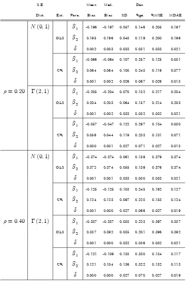
Table 1 summarizes the results for the OLS and CR estimators. As expected, the OLS

estimates of ₁₀ and ₂₀ are biased. The absolute value of this bias increases when

mov-ing from the low correlation to the high correlation state and is generally higher when

i;t standardized (2;1), the case re‡ecting a heavier-tailed process. In general, the

mag-nitude of this bias is large. The CR estimator displays notably less bias than its OLS

counterpart; however, the overall level of bias remains non-negligible, especially in the case

of fat-tailed errors.

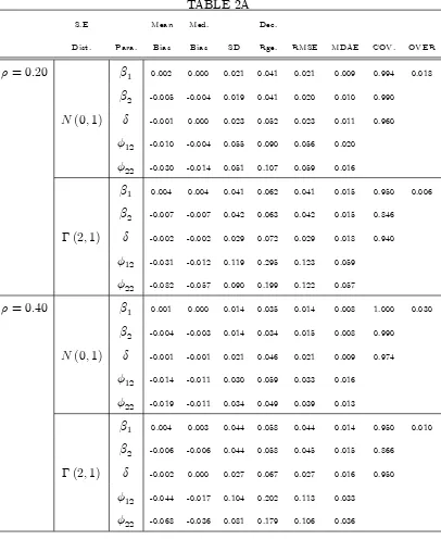
Table 2A summarizes the results for (15) whenK = 10. In the case where _i;t N(0; 1),

the estimates of 10 and 20 are unbiased. The nuisance parameters are slightly biased, but

this tendency does not e¤ect the estimates from the conditional mean. The coverage rates

tend to be too high and the rejection rates too low; however, the latter improves when

moving to the high correlation state. Overall, the CUE in (15) o¤ers a marked improvement

7_When_K_{= 10}_{, (15) contains}₄₀ _{moment conditions. When}_K_{= 20}_{, the number of moment conditions}

(14)

over both the OLS and CR estimators.

What is surprising in Table 2A is that (15) continues to produce unbiased estimates of ₁₀

and ₂₀ even when _i;t standardized (2;1). Irrespective of the correlation state, biases in

the nuisance parameters increase signi…cantly relative to the case where _i;t N(0; 1), but

this increase does not spill over onto the estimates from the conditional mean. Contrary to

what the theory predicts, therefore, it seems as if (15) remains consistent even if the fourth

moment of 2;t is not well de…ned. Also surprising is the …nding that coverage rates for b1

and b correspond to the chosen con…dence interval. The coverage rate for b₂, however, is

too low. In addition, the overidenti…cation test is signi…cantly undersized.

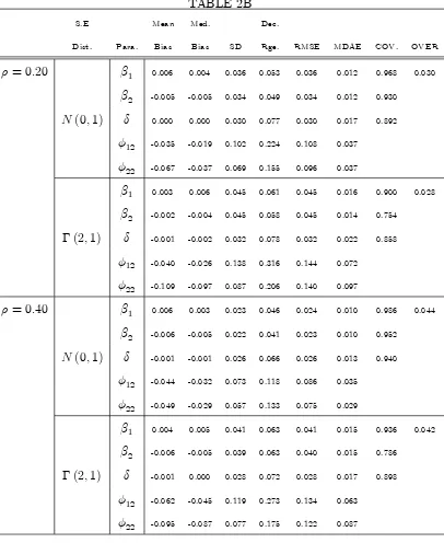
Table 2B summarizes results for the CUE when K = 20. In general, these results

(relative to those in Table 2A) con…rm the CUE as being robust to many moments bias.

For _i;t N(0; 1)across both correlation states, moving from K = 10 to K = 20 results in

diminished e¢ciency according to either the RMSE or MDAE. Coverage rates are generally

improved, however, and the rejection rates are much closer to being appropriately sized.

When i;t standardized (2;1), the same results emerge as in the case where K = 10.

Speci…cally, parameter estimates from the conditional mean remain unbiased even though

the nuisance parameters display non-negligible bias, which, relative to the case whereK = 10,

is more severe. There is also a noticeable deterioration in coverage rates, counter-balanced

against a marked improvement in rejection rates.

5. CAPM Betas

This section uses the CUE from section 3 to estimate CAPM betas for size, B/M, and

momentum portfolios following the example in section 1.2. These portfolios are studied

because they re‡ect the size, value, and momentum "premiums" that empirical applications

of the CAPM struggle to explain. The returns are measured weekly (in percentage terms)

from 10/6/67 through 9/28/07. Test results consider 20- and 10-year subperiods of this

overall date range. The daily 25 size-B/M and 25 size-momentum return …les (each 5 5

(15)

the NYSE, AMEX, and NASDAQ exchanges are used to construct the weekly return series.8

The size portfolios considered are "Small," "Mid," and "Large." "Small" is the average of the

…ve low market-cap portfolios, "Mid" the average of the …ve medium market-cap portfolios,

and "Big" the average of the …ve large market-cap portfolios. The B/M portfolios considered

are "Value," Neutral," and "Growth." Value" is the average of the …ve high B/M portfolios,

"Neutral" the average of the …ve middle B/M portfolios, and "Growth" the average of the …ve

low B/M portfolios.9 Finally, the momentum portfolios considered are "Losers," "Draws,"

and "Winners." "Losers" is the average of the …ve low return-sorted portfolios, "Neutral"

the average of the …ve middle return-sorted portfolios, and "Winners" the average of the

…ve high return-sorted portfolios. The proxy return for the true market return is the CRSP

value-weighted index return formed from all securities traded on the NYSE, AMEX, and

NASDAQ exchanges. Excess returns are calculated using the one-month Treasury bill rate

from Ibbotson Associates.

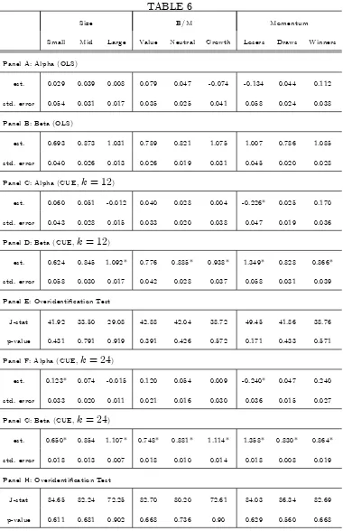
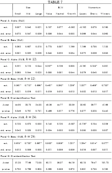
The most glaring take-away from Table 3, which summarizes estimation results for

re-turns measured between 10/6/67 and 9/25/87, is that di¤erences in beta estimates between

OLS and the CUE are large (i.e., of economic signi…cance) and statistically signi…cant.10

Moreover, this result is not impacted by the lag length chosen for the CUE. Since Theorem

1 nests the case of a zero covariance between structural errors–which, in the context of (7),

means that there is no measurement error in the market return–this …nding strongly suggests

that the standard approach to estimating beta is biased. This …nding is further supported by

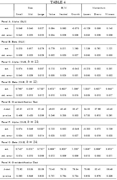
Table 4, which summarizes estimation results over the more-recent period 11/6/87 - 9/28/07,

and by Tables 5–7, which consider ten-year subperiods of the two date ranges considered in

Tables 3 and 4, respectively.11

Across the di¤erent portfolios, one can also observe an increase in the dispersion of the

8_{These return …les are available on Kenneth French’s website. Weekly returns are utilized because the}

CUE, which is based on higher moments, bene…ts from many observations in terms of …nite sample per-formance. Weekly returns are selected over daily returns because the former reduces day-of-the-week and weekend e¤ects as well as the e¤ects of nonsynchronus trading and bid-ask bounce.

9_{De…nitions for the "Small," "Large," "Value," and "Growth" portfolios are taken from Lewellen and}

Nagel (2006).

10_{Statistical signi…cance is determined using 95% con…dence intervals constructed from the standard errors}

of the CUE, which are consistent given general forms of heteroskedasticity and autocorrelation of the …rst order (i.e.,L= 2_).

(16)

beta estimates obtained using the CUE relative to OLS. Moreover, this increased dispersion

does not seem to link to imprecision in the individual beta estimates, since the standard

errors for the CUE are, at least, comparable in magnitude to their OLS counterparts. The

implication, therefore, is that the beta estimates obtained under the CUE display elevated

cross-sectional variation. In empirical asset pricing, betas obtained from time-series

regres-sions are important for their assumed role in pricing expected returns in the cross-section. A

well known empirical feature of cross-sectional expected returns is that (1) they tend to

ex-hibit substantial variation, and (2) their associated betas vary correspondingly little (minor

variations in betas cross-sectionally is evidenced in the …rst two panels of the Tables). This

second feature explains the poor empirical performance of the CAPM, which uses individual

asset sensitivities to the market return as its single pricing factor. Tables 3–7 suggest that

this poor performance may be overstated; using consistent beta estimates may improve the

ability of these estimates to explain variation in expected returns cross-sectionally.

Di¤erences in alpha estimates between the CUE and OLS appear decidedly more muted.

With minor exceptions, these estimates are statistically indistinguishable for the two

20-year time periods considered (see Tables 3 and 4). For the 10-20-year subperiods, however,

statistically distinct alpha estimates do arise, and, when they do, increases in their magnitude

(in absolute terms) under the CUE tend to explain the di¤erence, as opposed to reductions

in standard errors.

6. Conclusion

This paper presents a new method for estimating the linear triangular system, one which

does not rely upon the existence of outside instruments for identi…cation but, rather, a

particular parametric form for the CH in the structural errors. This parametric form is

common to empirical asset pricing speci…cations and tests. The estimator is shown to display

the usual pT-asymptotics and is robust to many (potentially weak) moments bias. It also

economizes on the number of nuisance parameters out of the CH process that need to be

estimated.

The estimator is applied to estimating market betas in a CAPM setting. The resulting

(17)

increased cross-sectional variation. The two-pass method of Fama and MacBeth (1973) for

testing asset pricing models relies upon time series beta estimates from the …rst pass. Works

reliant upon this method have found the risk premium associated with these …rst-pass betas

to be near zero or even negative (see, e.g., Jagannathan and Wang 1996 and Lettau and

Ludvigson 2001). Inconsistent beta estimates from the …rst pass will a¤ect the cross-sectional

results from the second pass and may explain these counter-intuitive results. Increased

cross-sectional variation in consistent beta estimates is a promising …nding that supports this

conjecture because of the empirical properties of cross-sectional expected returns.

Appendix

PROOF OF THEOREM 1: Given (14), …rst consider the case wherei=j =l =m = 2.

Then

Cov 2₂_;t; U₂₂_;t ₂ = ₂₂_;₀Cov 2₂_;t; U₂₂_;t ₁ ; (17)

which identi…es ₂₂_;₀ as

22;0 = Cov 22;t; U22;t 1

0

Cov 2₂_;t; U₂₂_;t ₁ 1Cov 2₂_;t; U₂₂_;t ₁ 0Cov 2₂_;t; U₂₂_;t ₂ :

Next leti= 1,j = 2, and l=m= 2. In this case,

Cov ₁_;t ₂_;t; U₂₂_;t ₂ = ₁₂_;₀Cov ₁_;t ₂_;t; U₂₂_;t ₁ ;

the reduced form of which is

Cov R₁_;t ₂_;t; U₂₂_;t ₂ = ₁₂_;₀Cov R₁_;t ₂_;t; U₂₂_;t ₁ + ₂_;₀ ₂₂_;₀ ₁₂_;₀ Cov 2₂_;t; U₂₂_;t ₁ ;

(18)

given (12) and (17). Finally, leti=l = 1 and j =m= 2. Then

(18)

the reduced form of which simpli…es to

Cov R₁_;t ₂_;t; U₁₂(R_;t) ₂ = ₁₂_;₀Cov R₁_;t ₂_;t; U₁₂(R_;t) ₁ + ₂_;₀ ₂₂_;₀ ₁₂_;₀ Cov 2₂_;t; U₁₂(R_;t) ₁ ;

(19)

given (12), (17), (18), and the fact that

Cov 2₂_;t; U₁₂(R_;t) ₂ = ₂₂_;₀Cov 2₂_;t; U₁₂(R_;t) ₁ :

Given (18) and (19), ₂

4 Cov R1;t 2;t; U

(R) 12;t 2

Cov R₁_;t ₂_;t; U₂₂_;t ₂

3

5= _R ;

where =h ₁₂_;₀ ₂_;₀ ₂₂_;₀ ₁₂_;₀ i

0

. Given A4, is identi…ed as

= 0_R _R 0_R

2

4 Cov R1;t 2;t; U

(R) 12;t 2

Cov R₁_;t ₂_;t; U₂₂_;t ₂

3 5;

from which ₁₂_;₀ is identi…ed, and ₂_;₀ is identi…ed conditional on the identi…cation

of both ₂₂_;₀ and ₁₂_;₀ and given A2. Finally, given A1, ₁_;₀ is identi…ed as ₁_;₀ =

E[X_tX0

t]

1

E X_t Y₁_;t Y₂_;t ₂_;₀ .

PROOF OF THEOREM 2: Given A6(ii), X_{t i;t} is uniformly integrable. A6(i) and

A6(ii), therefore, allow of an application of Theorem 1 in Andrews (1988), which

es-tablishes Result R1: T 1P

t

X_{t i;t} _!p 0. Next, recursive substitution into (13) produces

z_ij;₀_t =

1

P

p=0 p

W_{ij;t p}; (20)

where ₀ = 1 and _p = a_ij;₀ _ij;p ₀1 ₈ p 1. Since _p 1_p₌₀ is absolutely summable

given A2 and A3, and E W_ij;t 2 is …nite given A3, _fZij;t_g is an L1 _{mixingale that is}

uniformly integrable. As a consequence, Theorem 1 of Andrews (1988) applies again

to establish result R2: T 1P_Z

ij;t p

(19)

v_t;k is a L1 _{mixingale since} _Eh _W

ij;t

2i

is …nite (see Hamilton 1994 p. 192-93 for

a closely related proof). This result together with A6(iii) and R2 establishes Result

R3: T 1P

t

z_ij;tz_{lm;t k} _!p E z_ij;₀_tz_lm;₀_{t k} . Given results R1–R3, _bg( ) _!p g( ). Since

T p

! 0 by assumption,bg( )

0

T bg( ) p

!g( )0 ₀g( )by continuity of multiplication. Finally, given Theorem 1, g( )0 ₀g( ) is uniquely minimized at = ₀.

PROOF OF THEOREM 3: Using well known results on derivatives of inverse matrices,

the …rst order conditions for (15) with _T = b( ) 1 are

b

G b

0

b( ) 1 _bg b

0

b b 1b b b b 1 _bg b = 0:

Multiplying this expression by pT and expanding _bg b around ₀ produces

p

T b ₀ = G( ₀)0 ( ₀) 1G( ₀) 1G( ₀)0 ( ₀) 1pT_bg( ₀);

given A7(iv) and the following Results: (R4)_bg b _!p g( ₀) = 0, b b _!p ( ₀), and

b

G b _!p G( ₀) given Theorem 2 (speci…cally, Gb b _!p G( ₀) from the mixingale

and uniform integrability properties of A6); (R5) b b 1 _!p ( ₀) 1 given Theorem

2, A7(ii), A7(iii), and Lemma 4.3 of Newey and McFadden (1994) applied toa(z; ) =

g_{t s}( )g_t( )0

, where A7(iii) replaces the reliance on Khintchine’s law of large numbers

within the proof of this Lemma. Next, given absolute summability of _p 1_p₌₀ (see the

proof of Theorem 2), _fzij;0tg and vt;k are L2 mixingales, since E

h

W_ij;t 4i is …nite

under A7(ii). This result together with A7(i) establishes theL2 _{mixingale property for}

fg_t( ₀)_g, which satis…es the …rst element of Assumption 1 in De Jong (1997). Since the remaining elements hold under A7(v), pT_bg( ₀)_!d N(0; ( ₀)) by Theorem 1 of

the aforementioned work, where ( ₀) is …nite by A7(ii). The statement in (16) then

(20)

References

[1] Andrews, D.W.K., 1988, Laws of large numbers for dependent non-identically distrib-uted random variables, Econometric Theory, 4, 458-467.

[2] Baillie, R.T., and H. Chung, 2001, Estimation of GARCH models from the autocorre-lations of the squares of a process, Journal of Time Series Analysis, 22, 631-650.

[3] Bollerslev, T., 1986, Generalized autoregressive conditional heteroskedasticity, Journal of Econometrics, 31, 307–327.

[4] Bollerslev, T., 1988, On the correlation structure for the generalized autoregressive conditional heteroskedastic process, Journal of Time Series Analysis, 9, 121-131.

[5] Bollerslev, T., 1990, Modelling the coherence in short run nominal exchange rates: a multivariate generalized ARCH model, Review of Economics and Statistics, 72, 498-505.

[6] Bollerslev, T., R.F Engle and J.M. Wooldridge, 1988, A capital asset pricing model with time-varying covariances, Journal of the Political Economy, 96, 116-131.

[7] Carrasco, M. and X. Chen, 2002, Mixing and moment properties of various GARCH and stochastic volatility models, Econometric Theory, 18, 17-39.

[8] Cragg, J. and S. Donald, 1997, Inferring the rank of a matrix, Journal of Econometrics, 76, 223-250.

[9] Engle, R.F and K.F. Kroner, 1995, Multivariate simultaneous generalized GARCH, Econometric Theory, 11, 121-150.

[10] Fama, E.F. and J. MacBeth, 1973, Risk, return and equilibrium: empirical tests, Journal of Political Economy, 81, 607-636.

[11] Hamilton, J.D., 1994, Time series analysis, Princeton University Press.

[12] Han, C. and P.C.B. Phillips, 2006, GMM with many moment conditions, Econometrica, 74, 147-192.

[13] Hansen, L.P., J. Heaton and A. Yaron, 1996, Finite-sample properties of some alterna-tive GMM estimators, Journal of Business and Economic Statistics, 14, 262-280.

[14] Hansen, P.R. and A. Lunde, 2005, A forecast comparison of volatility models: does anything beat a GARCH(1,1)?, Journal of Applied Econometrics, 20, 873-889.

[15] He, C. and T. Teräsvirta, 1999, Properties of moments of a family of GARCH processes, Journal of Econometrics, 92, 173-192.

(21)

[17] Kristensen, D. and O. Linton, 2006, A closed-form estimator for the GARCH(1,1)-model, Econometric Theory, 22, 323-327.

[18] Klein, R. and F. Vella, 2010, Estimating a class of triangular simultaneous equations models without exclusion restrictions, Journal of Econometrics, 154, 154-164.

[19] Lettau, M. and S. Ludvigson, 2001, Resurrecting the (C)CAPM: a cross-sectional test with risk premia that are time varying, Journal of Political Economy, 109, 1238-1287.

[20] Lewbel, A., 2010, Using heteroskedasticity to identify and estimate mismeasured and endogenous regressor models, Journal of Business and Economic Statistics, forthcoming.

[21] Lewellen, J. and S. Nagel, 2006, The conditional CAPM does not explain asset-pricing anomalies, Journal of Financial Economics, 82, 289-314.

[22] Lintner, J., 1965, The valuation of risky assets and the selection of risky investments in stock portfolios and capital budgets," Review of Economics and Statistics, 47, 13–37.

[23] Meng, J.G., G. Hu and J. Bai, 2011, OLIVE: a simple method for estimating betas when feactors are measured with error, Journal of Financial Research, 34, 27-60.

[24] Newey, W.K. and D. McFadden, 1994, Large sample estimation and hypothesis testing, in R.F. Engle and D. McFadded, eds, Handbook of Econometrics, Vol. 4, Amsterdam North Holland, chapter 36, 2111-2245.

[25] Newey, W.K. and R.J. Smith, 2004, Higher order properties of GMM and generalized empirical likelihood estimators, Econometrica, 72, 219-255.

[26] Newey, W.K and F. Windmeijer, 2009, Generalized method of moments with many weak moment conditions, Econometrica, 77, 687-719.

[27] Prono, T., 2010, GARCH-based identi…cation and estimation of triangular systems, unpublished manuscript.

[28] Rigobon, R., 2003, Identi…cation through heteroskedasticity, Review of Economics and Statistics, 85, 777-792.

[29] Rigobon, R. and B. Sack, 2003, Measuring the response of monetary policy to the stock market, Quarterly Journal of Economics, 118, 639-669.

[30] Roll, R., 1977, A critique of the asset pricing theory’s tests: part I, Journal of Financial Economics, 4, 129–176.

[31] Rummery, S., F. Vella and M. Verbeek, 1999, Estimating the returns to education for Australian youth via rank-order instrumental variables, Labour Economics, 6, 491-507.

(22)

[33] Sharpe, W.F., 1964, Capital asset prices: a theory of market equilibrium under condi-tions of risk, Journal of Finance, 19, 425–442.

[34] Stock, J. and J. Wright, 2000, GMM with weak identi…cation, Econometrica, 68, 1055-1096.

[35] Vella, F. and M. Verbeek, 1997, Rank order as an instrumental variable, unpublished manuscript.

(23)

[image:23.612.120.493.89.658.2]

TABLE 1

S.E Mean Med. Dec.

Dist. Est. Para. Bias Bias SD Rge. RMSE MDAE

N(0;1) ₁ -0.196 -0.197 0.057 0.146 0.205 0.197

OLS ₂ 0.195 0.196 0.048 0.119 0.200 0.196

0.002 0.003 0.033 0.081 0.033 0.021

1 -0.066 -0.064 0.107 0.257 0.125 0.081

CR ₂ 0.064 0.064 0.100 0.248 0.119 0.077

0.001 0.002 0.026 0.067 0.026 0.018

= 0:20 (2;1) ₁ -0.205 -0.204 0.070 0.182 0.217 0.204

OLS ₂ 0.204 0.203 0.064 0.157 0.214 0.203

0.001 0.002 0.033 0.082 0.032 0.021

1 -0.057 -0.047 0.122 0.297 0.134 0.080

CR ₂ 0.056 0.044 0.119 0.283 0.131 0.071

0.000 0.001 0.027 0.071 0.027 0.018

N(0;1) 1 -0.374 -0.374 0.061 0.159 0.379 0.374

OLS ₂ 0.372 0.374 0.055 0.139 0.376 0.374

0.001 0.001 0.033 0.080 0.033 0.021

1 -0.125 -0.125 0.103 0.245 0.162 0.127

CR ₂ 0.124 0.123 0.097 0.228 0.158 0.124

0.001 0.000 0.027 0.066 0.027 0.019

= 0:40 (2;1) 1 -0.387 -0.387 0.088 0.223 0.397 0.387

OLS ₂ 0.387 0.392 0.085 0.201 0.396 0.392

0.001 0.000 0.032 0.086 0.032 0.021

1 -0.121 -0.109 0.138 0.330 0.184 0.117

CR ₂ 0.121 0.104 0.136 0.322 0.182 0.113

0.000 0.000 0.027 0.070 0.027 0.019

(24)

[image:24.612.105.511.76.573.2]

TABLE 2A

S.E Mean Med. Dec.

Dist. Para. Bias Bias SD Rge. RMSE MDAE COV. OVER

= 0:20 ₁ 0.002 0.000 0.021 0.041 0.021 0.009 0.994 0.018

2 -0.005 -0.004 0.019 0.041 0.020 0.010 0.990

N(0;1) -0.001 0.000 0.023 0.052 0.023 0.011 0.960

12 -0.010 -0.004 0.055 0.090 0.056 0.020

22 -0.030 -0.014 0.051 0.107 0.059 0.016

1 0.004 0.004 0.041 0.062 0.041 0.015 0.950 0.006

2 -0.007 -0.007 0.042 0.063 0.042 0.015 0.846

(2;1) -0.002 -0.002 0.029 0.072 0.029 0.018 0.940

12 -0.031 -0.012 0.119 0.295 0.123 0.059

22 -0.082 -0.057 0.090 0.199 0.122 0.057

= 0:40 1 0.001 0.000 0.014 0.035 0.014 0.008 1.000 0.030

2 -0.004 -0.003 0.014 0.034 0.015 0.008 0.990

N(0;1) -0.001 -0.001 0.021 0.046 0.021 0.009 0.974

12 -0.014 -0.011 0.030 0.059 0.033 0.016

22 -0.019 -0.011 0.034 0.049 0.039 0.013

1 0.004 0.003 0.044 0.058 0.044 0.014 0.950 0.010

2 -0.006 -0.006 0.044 0.058 0.045 0.015 0.866

(2;1) -0.002 0.000 0.027 0.067 0.027 0.016 0.950

12 -0.044 -0.017 0.104 0.202 0.113 0.033

22 -0.068 -0.036 0.081 0.179 0.106 0.036

Notes: Simulations are conducted using 1,000 observations across 500 trials. For the CUE,k= 10, and

(25)

[image:25.612.105.511.77.573.2]

TABLE 2B

S.E Mean Med. Dec.

Dist. Para. Bias Bias SD Rge. RMSE MDAE COV. OVER

= 0:20 ₁ 0.006 0.004 0.036 0.053 0.036 0.012 0.968 0.030

2 -0.005 -0.005 0.034 0.049 0.034 0.012 0.930

N(0;1) 0.000 0.000 0.030 0.077 0.030 0.017 0.892

12 -0.035 -0.019 0.102 0.224 0.108 0.037

22 -0.067 -0.037 0.069 0.155 0.096 0.037

1 0.003 0.006 0.045 0.061 0.045 0.016 0.900 0.028

2 -0.002 -0.004 0.045 0.058 0.045 0.014 0.754

(2;1) -0.001 -0.002 0.032 0.078 0.032 0.022 0.858

12 -0.040 -0.026 0.138 0.316 0.144 0.072

22 -0.109 -0.097 0.087 0.206 0.140 0.097

= 0:40 1 0.006 0.003 0.023 0.046 0.024 0.010 0.986 0.044

2 -0.006 -0.005 0.022 0.041 0.023 0.010 0.952

N(0;1) -0.001 -0.001 0.026 0.066 0.026 0.013 0.940

12 -0.044 -0.032 0.073 0.118 0.086 0.035

22 -0.049 -0.029 0.057 0.133 0.075 0.029

1 0.004 0.005 0.041 0.063 0.041 0.015 0.936 0.042

2 -0.006 -0.005 0.039 0.063 0.040 0.015 0.786

(2;1) -0.001 0.000 0.028 0.072 0.028 0.017 0.898

12 -0.062 -0.045 0.119 0.273 0.134 0.063

22 -0.095 -0.087 0.077 0.175 0.122 0.087

Notes: Simulations are conducted using 1,000 observations across 500 trials. For the CUE,k= 20, and

(26)

TABLE 3

Size B/M Momentum

Small Mid Large Value Neutral Growth Losers Draws Winners

Panel A: Alpha (OLS)

est. 0.045 0.060 0.016 0.113 0.053 -0.053 -0.106 0.045 0.132

std. error 0.045 0.026 0.013 0.033 0.023 0.028 0.043 0.022 0.033

Panel B: Beta (OLS)

est. 0.925 0.953 0.950 0.890 0.882 1.196 1.152 0.898 1.061

std. error 0.030 0.019 0.008 0.022 0.017 0.020 0.027 0.013 0.032

Panel C: Alpha (CUE,k = 12)

est. 0.069 0.075 0.021 0.130 0.069 -0.043 -0.186* 0.053 0.197

std. error 0.041 0.025 0.011 0.030 0.022 0.025 0.037 0.020 0.040

Panel D: Beta (CUE,k = 12)

est. 0.761* 0.817* 0.902* 0.724* 0.755* 1.117* 1.376* 0.860* 0.628*

std. error 0.024 0.013 0.007 0.016 0.011 0.016 0.021 0.012 0.017

Panel E: Overidenti…cation Test

J-stat 33.44 37.02 41.48 33.13 33.72 30.49 32.87 36.00 33.94

p-value 0.793 0.648 0.450 0.804 0.783 0.885 0.813 0.692 0.775

Panel F: Alpha (CUE,k= 24)

est. 0.086 0.084 0.018 0.138 0.074 -0.045 -0.195* 0.046 0.187

std. error 0.036 0.021 0.009 0.026 0.018 0.021 0.033 0.018 0.030

Panel G: Beta (CUE,k= 24)

est. 0.715* 0.753* 0.908* 0.694* 0.751* 1.110* 1.368* 0.846* 0.615*

std. error 0.014 0.008 0.004 0.010 0.018 0.009 0.012 0.007 0.011

Panel H: Overidenti…cation Test

J-stat 72.43 80.74 83.76 76.76 73.61 74.59 62.62 68.54 86.82

p-value 0.899 0.722 0.637 0.819 0.880 0.863 0.985 0.947 0.546

(27)

[image:27.612.116.500.73.662.2]

TABLE 4

Size B/M Momentum

est. 0.049 0.040 0.027 0.094 0.063 -0.070 -0.129 0.059 0.148

std. error 0.048 0.028 0.023 0.034 0.026 0.036 0.058 0.026 0.039

Panel B: Beta (OLS)

est. 0.810 0.917 0.879 0.779 0.811 1.160 1.139 0.761 1.121

std. error 0.039 0.023 0.029 0.032 0.020 0.027 0.050 0.028 0.038

Panel C: Alpha (CUE,k= 12)

est. 0.074 0.055 0.057 0.118 0.079 -0.048 -0.215 0.082 0.201

std. error 0.040 0.026 0.018 0.030 0.025 0.031 0.050 0.023 0.032

Panel D: Beta (CUE,k= 12)

est. 0.760* 0.829* 0.735* 0.615* 0.652* 1.206* 1.358* 0.631* 0.943*

std. error 0.023 0.018 0.012 0.018 0.015 0.015 0.035 0.013 0.017

J-stat 42.51 42.18 31.45 46.82 48.48 38.47 34.88 37.69 45.48

p-value 0.406 0.420 0.859 0.246 0.205 0.583 0.738 0.618 0.291

est. 0.074 0.049 0.058* 0.122 0.082 -0.046 -0.202 0.072 0.189

std. error 0.034 0.023 0.014 0.025 0.021 0.027 0.038 0.019 0.028

Panel G: Beta (CUE,k = 24)

est. 0.742* 0.818* 0.781* 0.609* 0.623* 1.220* 1.356* 0.606* 0.918*

std. error 0.014 0.010 0.006 0.012 0.009 0.009 0.018 0.008 0.011

J-stat 72.92 83.35 83.89 78.43 79.13 79.54 70.60 82.41 86.49

p-value 0.892 0.649 0.633 0.781 0.764 0.754 0.925 0.676 0.556

(28)

TABLE 5

Size B/M Momentum

est. 0.091 0.081 -0.002 0.130 0.068 -0.045 -0.081 0.048 0.141

std. error 0.053 0.031 0.016 0.039 0.025 0.036 0.052 0.026 0.046

Panel B: Beta (OLS)

est. 0.826 0.922 0.972 0.803 0.873 1.177 1.001 0.859 1.110

std. error 0.040 0.024 0.010 0.033 0.018 0.025 0.035 0.017 0.041

est. 0.096 0.069 0.023 0.207* 0.062 -0.086 -0.175* 0.037 0.178

std. error 0.040 0.026 0.016 0.033 0.020 0.032 0.046 0.021 0.037

est. 0.947* 0.974* 0.816* 0.575* 0.886 1.421* 1.287* 0.874 1.107

std. error 0.027 0.019 0.008 0.020 0.015 0.019 0.021 0.014 0.026

J-stat 31.87 31.49 37.34 39.55 34.84 36.387 44.13 41.27 29.14

p-value 0.846 0.858 0.634 0.535 0.740 0.676 0.341 0.459 0.917

est. 0.061 0.069 0.027 0.184* 0.075 -0.131* -0.188* 0.041 0.185

std. error 0.033 0.019 0.014 0.027 0.016 0.026 0.036 0.016 0.031

est. 0.959* 0.983* 0.794* 0.579* 0.890* 1.440* 1.205* 0.875* 1.137

std. error 0.017 0.010 0.004 0.012 0.008 0.012 0.012 0.007 0.016

J-stat 73.55 72.20 84.14 81.37 77.25 79.88 79.81 77.89 74.79

p-value 0.881 0.903 0.626 0.705 0.808 0.745 0.747 0.794 0.859

(29)

[image:29.612.118.498.73.661.2]

TABLE 6

Size B/M Momentum

est. 0.029 0.039 0.008 0.079 0.047 -0.074 -0.134 0.044 0.112

std. error 0.054 0.031 0.017 0.035 0.025 0.041 0.058 0.024 0.038

Panel B: Beta (OLS)

est. 0.693 0.873 1.031 0.789 0.821 1.075 1.007 0.786 1.085

std. error 0.040 0.026 0.013 0.026 0.019 0.031 0.045 0.020 0.028

Panel C: Alpha (CUE,k= 12)

est. 0.060 0.051 -0.012 0.040 0.028 0.004 -0.226* 0.025 0.170

std. error 0.043 0.028 0.015 0.033 0.020 0.038 0.047 0.019 0.036

Panel D: Beta (CUE,k= 12)

est. 0.624 0.845 1.092* 0.776 0.885* 0.938* 1.349* 0.828 0.866*

std. error 0.058 0.030 0.017 0.042 0.028 0.037 0.058 0.031 0.039

J-stat 41.92 33.50 29.08 42.88 42.04 38.72 49.45 41.86 38.76

p-value 0.431 0.791 0.919 0.391 0.426 0.572 0.171 0.433 0.571

est. 0.123* 0.074 -0.015 0.120 0.054 0.009 -0.240* 0.047 0.240

std. error 0.033 0.020 0.011 0.021 0.016 0.030 0.036 0.015 0.027

Panel G: Beta (CUE,k = 24)

est. 0.650* 0.854 1.107* 0.748* 0.881* 1.114* 1.358* 0.830* 0.864*

std. error 0.018 0.013 0.007 0.018 0.010 0.014 0.018 0.008 0.019

J-stat 84.65 82.24 72.25 82.70 80.20 72.61 84.03 86.34 82.69

p-value 0.611 0.681 0.902 0.668 0.736 0.90 0.629 0.560 0.668

(30)

[image:30.612.117.501.73.662.2]

TABLE 7

Size B/M Momentum

est. 0.087 0.048 0.021 0.107 0.077 -0.052 -0.102 0.070 0.190

std. error 0.078 0.047 0.039 0.056 0.044 0.058 0.099 0.044 0.068

Panel B: Beta (OLS)

est. 0.863 0.937 0.810 0.775 0.807 1.199 1.199 0.750 1.138

std. error 0.051 0.032 0.036 0.045 0.028 0.034 0.072 0.039 0.053

est. 0.221 0.110 0.044 0.207* 0.126 0.000 -0.161 0.155* 0.301

std. error 0.065 0.044 0.028 0.050 0.051 0.044 0.079 0.040 0.051

est. 0.561* 0.718* 0.696* 0.461* 0.398* 1.239* 1.337* 0.469* 0.783*

std. error 0.021 0.016 0.011 0.019 0.015 0.013 0.032 0.013 0.017

J-stat 44.00 35.78 34.55 40.36 44.77 33.89 38.62 39.77 41.66

p-value 0.346 0.701 0.751 0.499 0.317 0.776 0.577 0.525 0.442

est. 0.125 0.078 0.038 0.148 0.120 -0.057 -0.116* 0.104 0.229

std. error 0.043 0.035 0.018 0.034 0.033 0.030 0.050 0.030 0.037

est. 0.615* 0.738* 0.697* 0.503* 0.509* 1.231* 1.294* 0.514* 0.877*

std. error 0.013 0.009 0.005 0.011 0.009 0.009 0.016 0.007 0.011

J-stat 81.25 77.66 72.05 92.11 86.37 64.19 68.15 79.47 101.73

p-value 0.708 0.799 0.905 0.390 0.559 0.978 0.951 0.755 0.168