B Spline Collocation Method for Solving Singularly Perturbed Boundary Value Problems

http://www.scirp.org/journal/jamp ISSN Online: 2327-4379

ISSN Print: 2327-4352

B-Spline Collocation Method for Solving Singularly

Perturbed Boundary Value Problems

Bin Lin

School of Mathematics and Computation Science, Lingnan Normal University, Zhanjiang, China

Abstract

We use fifth order B-spline functions to construct the numerical method for solving singularly perturbed boundary value problems. We use B-spline collocation method, which leads to a tri-diagonal linear system. The accuracy of the proposed method is demonstrated by test problems. The numerical results are found in good agreement with exact solutions.

Keywords

Fifth Order B-Spline Functions, B-Spline Collocation Method, Singularly Perturbed Boundary Value Problems

1. Introduction

Consider following singularly perturbed boundary value problem

( )

( )

( )

( )

,

Ly x = −ε ′′y +p x y′+q x y= f x a< <x b (1)

with boundary conditions

( )

,

( )

,

( )

,

( )

y a =A y b =B y a′ =γ y b′ =δ (2)

where 0< <ε 1, ε is a small positive parameter, p x

( )

and q x

( )

are sufficiently

smooth real-valued functions. Typically, these problems arise very frequently in fluid dynamics, elasticity, quantum mechanics, chemical reactor theory and many other al-lied areas. Up to now, different numerical methods have been proposed by various au-thors [1]-[3] for this singularly perturbed problem arising in transport phenomena in chemistry and biology [4]. It is so attractive to mathematicians due to the fact that the solution exhibits a multi-scale character, i.e., there is a thin layer where the solution va-ries rapidly, while away from the layer the solution behaves regularly and vava-ries slowly. So the usual numerical treatment of singular perturbation problems gives rise to major

How to cite this paper: Lin, B. (2016) B-Spline Collocation Method for Solving Singularly Perturbed Boundary Value Prob-lems. Journal of Applied Mathematics and Physics, 4, 1699-1704.

http://dx.doi.org/10.4236/jamp.2016.49178

Received: July 18, 2016 Accepted: September 4, 2016 Published: September 7, 2016

Copyright © 2016 by author and Scientific Research Publishing Inc. This work is licensed under the Creative Commons Attribution International License (CC BY 4.0).

computational difficulties and fails to give accurate solutions.

B-spline functions are useful wavelet basis functions; the stiffness matrix is sparse when it is used as trial functions. B-splines were introduced by Schoenberg in 1946 [5]. Up to now, B-spline approximation method for numerical solutions has been re-searched by various researchers [6]-[8].

2. Description of the B-Spline Collocation Method

The expression of fifth order B-spline function is as follows:

( )

(

)

[

)

(

)

(

)

[

)

(

)

(

)

(

)

[

)

(

)

(

)

(

)

[

)

(

)

(

)

[

)

(

)

5 5 5

5 5 5

5 5 5 6 5 5 5

3 3, 2

3 6 2 2, 1

3 6 2 15 1 1, 0

3 ) 6 2 15 1 0,1

3 ) 6 2 1, 2

3 x

x x

x x x

N x x x x

x x x + − − + − + − − + − + + + − = − − − + − − − −

−

[

2, 3

)

0 others

             (3)

The fifth order B-spline function N6

( )

x is used to calculate in this work and

pos-sesses the following characters: piecewise smooth, compact support, Symmetry, rapidly decaying, differentiability, linear combination.

The region [a,b] is partitioned into uniformly sized finite elements of length h by the knots xj such that a=x0<x1<x2< ⋅⋅⋅ <xN =b with h=xj−xj−1, xj = +a jh,

1, 2, ,

j=  N. Let φm

( )

x be fifth order B-spline function with knots at the points xm,

0,1, ,

m=  N. The set of splines

{

φ φ φ φ−2, −1, 0, ,1,φ φN, N+1,φN+2

}

forms a basis for

functions defined over [a,b].

In the proposed algorithm, The fifth order B-spline function N6

( )

x is used as a

single mother wavelet, i.e. φ

( )

x =N6

( )

x and dilation and translation of mother

wavelet functions can construct any function of 2

( )

L R .

( )

( )

2

(

)

6

2

2 2

2

J

J J J k

k k k k J k

k k k k

x x

x k

S x c x c x k a a N

h

φ φ φ −₋−   − 

= = − = _{ }= _{ }

   

∑

∑

∑

∑

(4)

where _{1 2 , 2 , 2}J J J2 _.

k k k

h= x =k

a

= c

So the global approximation S x

( )

to the function y x

( )

can be written in terms

of the B-spline as follows

( )

2 6 2 N i i i x x

S x a N

h + =− −   = _{ }  

∑

, (5)

where h b a n

−

= , ai are unknown real coefficients.

Using the fifth order B-spline function and the approximate solution Equation (5), the nodal values S x

( )

j , S x′

( )

j and S′′

( )

xj at the node xj are given in terms of

( )

(

2 1 1 2

)

1

26 66 26

120

j j j j j j

S x = a₋ + a₋ + a + a₊ +a₊ (6)

( )

(

2 1 1 2

)

1

10 10

24

j j j j j

S x a a a a

h − − + +

′ = − − + + (7)

( )

2

(

2 1 1 2

)

1

2 6 2

6

j j j j j j

S x a a a a a

h − − + +

′′ = + − + + ₍₈₎

where the symbols ' and '' denote first and second differentiation with respect to x,

respectively.

Substituting Equations (6)-(8) into Equation (1) and Equation (2), we can obtain following linear equations

Ba=r (9)

where

( )

( )

( )

( )

(

)

T

2 2

0

120 , 24 , 120 , , 120 N , 24 ,120

r= y a hy a′ − h f ε  − h f ε hy b′ y b

(

)

T

2, 1, 0, 1, , N, N1, N 2

a= a₋ a₋ a a ⋅⋅⋅a a ₊ a ₊ , fi= f a

(

+ih

)

Note 6

j i i j x x N B h −   =    

2,0 1,0 0,0 1,0 2,0

2, 1, , 1, 2,

1 26 66 26 1 0

1 10 0 10 1 0

1 10 0 10 1

1 26 66 26 1

N N N N N N N N N N

LB LB LB LB LB

B

LB LB LB LB LB

− − − − + +    _{− −}        =       − −            where

(

)

(

)

2 2 2, 1, 2 2 , 1, 2 2,

20 5 , 40 50 26

120 66 , 40 50 26

20 5 , ,

j j j j j j j j

j j j j j j j

j j j j j j

LB hp h q LB hp h q

LB h q LB h p h q

LB h p h q p p a jh q q a jh

ε ε ε ε

ε ε ε

ε ε − − + + = + − = + − = − − = − − = − − = + = +

It is easily seen that the matrix B is strictly diagonally dominant and hence nonsin-gular. Since B is nonsingular, we can solve the system Ba=r for

2, 1, 0, 1, , N, N 1, N 2

a− a− a a  a a + a + . Hence the method of collocation using the fifth order

B-spline function N6

( )

x as a basis function applied to the singularly perturbed

boundary value problem has a unique solution S x

( )

given by Equation (5).

3. Numerical Results

In the section, we illustrate the numerical techniques discussed in the previous section by the following problems.

Example 1. Consider the convention-dominated equation:

(

)

1 0 1

y y y x

ε ′′ ′

with boundary conditions: y

( )

0 = y

( )

1 =0,

( )

(

2

)

(

1

) (

1 2

)

1 2

0 e 1 1 e e e

y′ =_λ λ − +λ − λ _ λ − λ ,

( )

(

2

)

1

(

1

)

2

(

1 2

)

1 2

1 e 1 e 1 e e e e

y′ =_λ λ − λ +λ − λ λ _ λ − λ .

The exact solution is given by

( )

(

_e2 _{1 e}

)

1x

(

_e1 _e2

) (

_{1 e}1

)

_e2x

(

_e1 _e2

)

₁

y x = λ − λ λ − λ + − λ λ λ − λ + (11)

where λ1= +

(

1 1 4+ ε

)

( )

2ε λ, 12= −

(

1 4+ ε

)

( )

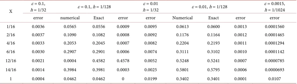
2ε .

Comparison of the numerical results and point-wise errors is given in Table 1. It observed that

1) when h decreases (i.e. collocation number increases) for fixed ε the point-wise errors decrease;

2) when ε decreases for fixed h the point-wise errors increase; 3) when ε =0.0015, x→1 the errors are very large.

Example 2. Solve the following non-homogeneous equation:

(

)

cosπ 0 1

y py y x x

ε ′′ ′

− + + = < < ₍₁₂₎

with boundary conditions

( )

0

( )

1 0

y = y = ,

( )

2

1 2

0 π e

y′ =b +Aλ λ+ B −λ ,

( )

1

1 2

1 π e

y′ = − +b Aλ λ +λ B.

The analytical solution is given by

( )

cosπ sinπ exp

( )

1 exp 2

(

1

)

y x =a x b+ x+A λx +B _−λ −x _ (13)

where

(

)

(

)

2

2 2

2 2 2 2 2 2

π 1 π

,

π π 1 π π 1

p

a b

p p

ε

ε ε

+

= =

+ + + + ,

(

)

(

1 22

)

(

1

( )

1 2

)

1 exp 1 exp

,

1 exp 1 exp

A a λ B a λ

λ λ λ λ

+ − +

= − =

− − − − .

And λ <1 0 and λ >2 0 are the real solutions of the characteristic equation 2

1 0

p

ελ λ

− + + = _.

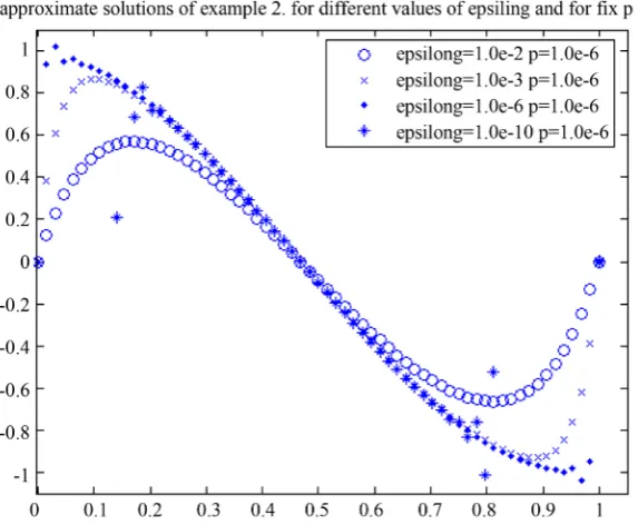
[image:4.595.45.554.562.707.2]

Approximation solutions for different values of ε and for fixed p are given in Fig-ure 1. It observed that

Table 1. Example 1. Comparison of results and point-wise errors.

X

ε = 0.1,

h = 1/32 ε = 0.1, h = 1/128

ε = 0.01

h = 1/32 ε = 0.01, h = 1/128

ε = 0.0015,

h = 1/1024

error numerical Exact error error Numerical Exact error error

1/16 0.0036 0.0565 0.0556 0.0009 0.0095 0.0613 0.0600 0.0013 0.0001560

2/16 0.0037 0.1090 0.1082 0.0008 0.0092 0.1176 0.1164 0.0012 0.0001465

4/16 0.0033 0.2053 0.2045 0.0007 0.0082 0.2204 0.2193 0.0011 0.0001294

6/16 0.0030 0.2907 0.2901 0.0006 0.0074 0.3111 0.3102 0.0010 0.0001142

12/16 0.0021 0.0004 0.4582 0.4578 0.0052 0.5248 0.5241 0.0007 0.0000785

14/16 0.0014 0.3984 0.3981 0.0003 0.0025 0.5801 0.5795 0.0006 0.0000693

[image:5.595.232.519.72.308.2]

Figure 1. Approximation solutions of example 2 for different values of epsilon g and for fixed p.

1) when 2

10

ε₌ − _and 3

10− , the approximation solutions are in good agreement

with exact solution; 2) when 6

10

ε ₌ − _and 10

10− , x→0 and x→1 the errors are

very large; 3) when ε decreases for fixed p the width of boundary layer becomes small and wave shape change more and more stiff at x=0 and x=1.

4. Conclusion

The numerical results show clearly the effect of ε on the boundary layer and the B-spline collocation method solving singular boundary value problems is relatively simple to collocate the solution at the mesh points. It is applicable technique and ap-proximates the exact solution very well.

Acknowledgements

The authors would like to thank the editor and the reviewers for their valuable com-ments and suggestions to improve the results of this paper. This work was supported by the Natural Science Foundation of Guangdong (No. 2015A030313827).

References

[1] Evrenosoglu, M. and Somali, S. (2008) Least Squares Methods for Solving Singularly Per-turbed Two-Point Boundary Value Problems Using Bezier Control Points. Applied

Ma-thematics Letters, 21, 1029-1032. http://dx.doi.org/10.1016/j.aml.2007.10.021

[2] Lin, B., Li, K.T. and Cheng, Z.X. (2009) B-Spline Solution of a Singularly Perturbed Boun-dary Value Problem Arising in Biology. Chaos, Solitons & Fractals, 42, 2934-2948.

http://dx.doi.org/10.1016/j.chaos.2009.04.036

mKdV-KS Equation. Chaos, Solitons & Fractals, 26, 1111-1118.

http://dx.doi.org/10.1016/j.chaos.2005.02.014

[4] Bigge, J. and Bohl, E. (1985) Deformations of the Bifurcation Diagram Due to Discretiza-tion. Mathematics of Computation, 45, 393-403.

http://dx.doi.org/10.1090/S0025-5718-1985-0804931-X

[5] De Boor, C. (1978) A Practical Guide to Splines. Springer-Verlag, Berlin.

http://dx.doi.org/10.1007/978-1-4612-6333-3

[6] Siddiqi, S.S. and Akram, G. (2007) Sextic Spline Solutions of Fifth Order Boundary Value Problems. Applied Mathematics Letters, 20, 591-597.

http://dx.doi.org/10.1016/j.aml.2006.06.012

[7] Caglar, H.N. and Caglar, S.H. (1997) The Numerical Solution of Fifth Order Boundary Value Problems with Sixth Degree B-Spline Functions. Applied Mathematics Letters, 12, 25-30. http://dx.doi.org/10.1016/S0893-9659(99)00052-X

[8] Cağlar, H., Özer, M. and Cağlar, N. (2008) The Numerical Solution of the One-Dimen- sional Heat Equation by Using Third Degree B-Spline Functions. Chaos, Solitons & Frac-tals, 38, 1197-1201.http://dx.doi.org/10.1016/j.chaos.2007.01.056

Submit or recommend next manuscript to SCIRP and we will provide best service for you:

Accepting pre-submission inquiries through Email, Facebook, LinkedIn, Twitter, etc. A wide selection of journals (inclusive of 9 subjects, more than 200 journals)

Providing 24-hour high-quality service User-friendly online submission system Fair and swift peer-review system

Efficient typesetting and proofreading procedure

Display of the result of downloads and visits, as well as the number of cited articles Maximum dissemination of your research work