Ev al u a ti o n of u n c e r t a i n ti e s i n
cl a s si c al a n d c o m p o n e n t ( blo c k e d
fo r c e ) t r a n sf e r p a t h a n a ly si s
(TPA)
M o o r h o u s e , AT, M e g g i t t , JWR a n d Ellio t t , AS
h t t p :// dx. d oi.o r g / 1 0 . 4 2 7 1 / 2 0 1 9-0 1-1 5 4 4
T i t l e
Ev al u a tio n of u n c e r t ai n ti e s in cl a s si c al a n d c o m p o n e n t
( blo c k e d fo r c e) t r a n sf e r p a t h a n a ly si s (TPA)
A u t h o r s
M o o r h o u s e , AT, M e g g i t t , JWR a n d Ellio t t , AS
Typ e
Ar ticl e
U RL
T hi s v e r si o n is a v ail a bl e a t :
h t t p :// u sir. s alfo r d . a c . u k /i d/ e p ri n t/ 5 2 9 2 7 /
P u b l i s h e d D a t e
2 0 1 9
U S IR is a d i gi t al c oll e c ti o n of t h e r e s e a r c h o u t p u t of t h e U n iv e r si ty of S alfo r d .
W h e r e c o p y ri g h t p e r m i t s , f ull t e x t m a t e r i al h el d i n t h e r e p o si t o r y is m a d e
f r e ely a v ail a bl e o nli n e a n d c a n b e r e a d , d o w nl o a d e d a n d c o pi e d fo r n o
n-c o m m e r n-ci al p r iv a t e s t u d y o r r e s e a r n-c h p u r p o s e s . Pl e a s e n-c h e n-c k t h e m a n u s n-c ri p t
fo r a n y f u r t h e r c o p y ri g h t r e s t r i c ti o n s .
Evaluation of uncertainties in classical and component (blocked force) transfer path
analysis (TPA)
A.T. Moorhouse1, J.W.R. Meggitt1, A.T. Elliott1
1Acoustics Research Centre, University of Salford, Greater Manchester, M5 4WT
Abstract
Transfer path analysis (TPA) has become a widely used diagnostic technique in the automotive and other sectors. In classic TPA, a two-stage measurement is conducted including operational and frequency response function (FRF) phases from which the contribution of various excitations to a target quantity, typically cabin sound pressure, are determined. Blocked force TPA (also called in situ Source Path Contribution Analysis, in-situ TPA and component TPA) is a development of the classic TPA approach and has been attracting considerable recent attention. Blocked force TPA is based on very similar two stage measurements to classic TPA but has two major advantages: there is no need to dismantle the vehicle and the blocked forces obtained are an independent property of the source component and are therefore transferrable to different assemblies. However, despite the now widespread reliance on classic TPA, and the increasing use of blocked force TPA in the automotive sector, it is rare to see any evaluation of the associated uncertainties. This paper therefore aims to summarize recent work and provide a guide to the evaluation of uncertainties in both forms of TPA. The various types of uncertainty are first categorized as, ‘model’, ‘source’ and ‘experimental’ uncertainties. Model uncertainties arise due to incomplete or inconsistent representation of the physical assembly by the measurements. Criteria are provided for evaluation of completeness in terms of measured quantities. Experimental and source uncertainties are evaluated through a first order propagation approach. Expressions are provided allowing the uncertainty in the target quantity to be estimated from measured quantities. Additional data storage and analysis is required but no additional measurements are needed over and above the usual TPA measurements. An illustrative example is provided.
1. Introduction
Transfer path analysis (TPA) has become a widely used diagnostic technique in the automotive industry, as well as in other industrial sectors [1]. The aim is to quantify the contribu-tions of various structural transmission paths to a vibro-acoustic target quantity, typically cabin sound pressure. This breakdown provides valuable information for engineers to influence e.g. cabin sound pressure through modification of structural com-ponents. Noise sources considered include road noise, engine noise as well as others. Airborne sources and transmission can be included in TPA, but the focus here is on structural transmis-sion. In this paper we consider the uncertainties and errors in two of the most widely used variants of TPA, namely classical [2, 3] (matrix inverse) and component (blocked force) TPA [4]. Other TPA variants, such as the mount stiffness method [1] and advanced TPA [5], are not considered although could be subject to a similar analysis.
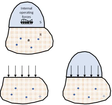
In both classical and blocked force TPA, the assembled ve-hicle is delineated into a source region, S, and a receiver region, R (see Figure 1). The source region contains all the source mechanisms of interest and frequently also includes some pas-sive structures. For road noise for example, the source region includes the tire-road contact patch, the tire, wheel, hub and parts of the suspension such as wishbones. All parts of the ve-hicle downstream of the source-receiver interface are consid-ered to belong to the receiver, which for road noise typically
includes the cabin, body, perhaps subframes and possibly some upper parts of the suspension. It is assumed that a set of forces act on the receiver region from the source region. Normally in TPA these forces are considered to act at discreet points but may include moments as well as ordinary forces. The aim of TPA is to quantify the contributions of each of the forces to the target quantity, P. Arguably, these are contributions rather than ‘transfer paths’ but we will continue to use the term transfer path analysis since this name has become widely adopted.
1.1. Measurements for TPA
A two-stage measurement process is needed for both classi-cal and blocked force TPA. The first phase is an operational test where the vehicle is run under appropriate load cycles while ac-celerations and sound pressures are recorded at various points on the structure and in the cabin. Essentially the same oper-ational test is used for both classical and blocked force TPA. A ‘passive’ measurement phase is then conducted with the ve-hicle at rest in which frequency response functions (FRFs) are measured, typically using excitation from a hammer. In clas-sical TPA, the source and receiver regions must be phyclas-sically separated for this phase so that the FRFs relate purely to the re-ceiver substructure. In blocked force TPA, the vehicle remains fully assembled and the FRFs therefore relate to the whole as-sembly.
inter-Figure 1: Schematic of measurement phases in TPA. Upper: operational test. Lower: FRF test for classical (left) and blocked force (right) TPA. S, R: source, receiver.a: operational accelerations. Dots and crosses: responses at indicator and target locations.
face, and the second a forward or prediction step to calculate the contribution of these forces to the target quantity. The above measurement approaches can provide invaluable diagnostic in-formation. However, they are known to be sensitive to measure-ment and other errors. It is perhaps surprising then that com-paratively little attention has been devoted to the treatment of uncertainties in TPA. Hence, the aim of this paper is to provide a guide to the evaluation of uncertainties in both classical and blocked force TPA. The emphasis will be on providing as com-prehensive a treatment as possible by bringing together already published results into a common framework. The reader will be referred to source publications for detailed derivations. In the following section we categorize the uncertainties affecting TPA as, ‘model’, ‘source’, ‘or ‘experimental’ uncertainties. ‘Model’ uncertainties are then discussed by considering the ‘complete-ness’ and ‘consistency’ with which the measurements are able to represent the physical test structure. Treatment of ‘source’ and ‘experimental’ uncertainties are then discussed and practi-cal methods for their evaluation are provided. These concepts are illustrated through a simulation example before a final sum-mary and conclusions.
2. Types of Uncertainty in TPA
In this section we provide a categorization of the various forms of error and uncertainty affecting TPA. First though, we define the essential TPA equations.
2.1. Classical and blocked force TPA
The inverse and prediction steps in TPA are encapsulated respectively by the following equations:
f=Y+a (1)
p=Hf (2)
In equation (1),a, is a vector of operational accelerations mea-sured at indicator positions, usually on or close to the source-receiver interface (see fig 1);f is an initially unknown vector of generalized forces acting at the interface degrees of freedom.
Yis a matrix of FRFs relating the indicator and interface de-grees of freedom and Y+ indicates the inverse of this matrix (a pseudo-inverse for non-square matrices and a conventional inverse for square matrices). The force vector calculated from equation (1) is taken as the input to the prediction step outlined in equation (2) wherepis a vector of (predicted) target quanti-ties, usually cabin pressure at various points andHis a matrix of FRFs relating target and interface degrees of freedom. All quantities are assumed to be in the frequency domain and the dependence on radian frequency W is omitted for clarity.
Both classical and blocked force TPA can be described in terms of these same equations. However, there are some dif-ferences in the interpretation of the quantities apart from the indicator accelerations A in equation (1) which are the same for both methods, being based on identical measurements [4]. In classical TPA, the FRF measurements are conducted with the source substructure removed and hence the matricesYandH
relate to the receiver substructure only. In this case, the forces obtained from the inverse step, equation (1), are the contact forces at the interface, in other words the forces exerted by the source on the receiver. On the other hand, in blocked force TPA, the source and receiver substructures remain attached for the FRF measurements, so the matricesYandHrelate to the whole assembly. In this case, the forces obtained are the blocked forces of the source [6]. The physical interpretation of the blocked forces is slightly more abstract than for the contact forces, however, this minor disadvantage is compensated by a significant benefit in that they are independent of the receiver structure and can hence be transferred to assemblies where the same source is mounted on different receivers. This advan-tage is one of the main reasons why blocked force TPA is cur-rently attracting interest. The inherent possibilities have been described in more detail elsewhere [1].
The ‘output’ of TPA depends on what it is being used for. As a diagnostic technique the desired quantities are the contri-butions to the target quantity, i.e. rewriting the righthand side of equation (2), the relative magnitudes of the terms in the sum (the transfer path contributions) are of primary interest:
p=X
i
Hifi (2a)
whereHiare the columns ofH. However, with blocked force
[image:3.595.50.278.78.292.2]Category Description
Model:
Completeness
Due to incomplete representation of all sig-nificant forces at the source-receiver inter-face
Consistency
Due to variations in system properties between the operational and passive test phases
Source Uncertainty inherent in the source
opera-tion
Experimental:
Measurement Due to noise in the measurement chain
Operator Due to random errors in location and direc-tion of forces during FRF measurement
2.2. Categories of Uncertainty
Meggitt et al.[7] have recently categorized the sources of uncertainty in inverse force identification as originating from the ‘model’, the ‘source’, and the ‘experiment’. These cate-gories have been slightly extended here for the context of TPA. The categories are summarized below and in table 1 and are described in more detail in the following two main sections.
‘Model’ uncertainty arises due to imperfect representation of the physical system by the measured data, for example due to inherent assumptions. A main cause is lack of ‘complete-ness’ in the representation of the interface, for example due to neglected degrees of freedom. Similarly, if the measurement points are not located at the actual location of the interface forces then an error can be expected. Strictly speaking, these are systematic errors rather than uncertainties but are an impor-tant reason (possibility the main reason) for poor results in TPA and so are included in this overview.
A further cause of ‘model’ error lies in lack of ‘consistency’ between the operational and FRF measurement phases, for ex-ample due to temperature variation or operating loads. Again, this is a systematic error rather than an uncertainty. Consistency is classed here as a form of model uncertainty, although it could be argued that it is a separate category.
‘Source’ uncertainties arise due to the variations (assumed random) in the operation of the source. Source uncertainties are handled here in a conventional way by obtaining a number of samples during operation from which estimates of statistical properties (mean and variance) are obtained. As an example, it is clear that road noise is a statistical source that requires repeated measurements over time with appropriate statistical treatment of the data.
‘Experimental’ uncertainties were defined by Meggitt et al [7] as comprising ‘measurement’ and ‘operator’ uncertainty. Measurement uncertainty consists of uncorrelated noise in the measurement chain which could originate from electrical noise in instruments or uncorrelated background noise in the acceler-ation signals,a. Again, this is handled by repeating measure-ments so as to obtain a set of samples from which statistical properties are derived. ‘Operator’ uncertainty arises due to a lack of repeatability in the measurement of FRFs. Assuming
that the structures are excited by an instrumented hammer dur-ing the FRF measurement phase, then differences (assumed to be random) are expected from one hit to the next both in the po-sition and direction of the hit. (Note that differences in strength of the hit are not considered a source of uncertainty because, assuming linearity, the FRFs are normalized to the input force). It is normal practice to average the results of several hammer hits to obtain average FRFs, however, we recommend here that the individual FRFs obtained with each hit are retained so as to allow calculation of the variance (and covariance) in addition to the mean during postprocessing. Further details are provided later.
In the following we discuss first model uncertainty before then going on to present a framework for evaluation of all other types of uncertainty.
3. Model Uncertainty
An important cause of error in TPA lies in what we are terming ‘model’ uncertainty. Two categories of model uncer-tainty have been identified above, relating to completeness and consistency.
3.1. Completeness
Although TPA is an experimental technique, it is neverthe-less necessary to adopt a ‘model’ of the physical system, com-prising various assumptions, so that it can be represented by measured data. For TPA, a crucial aspect of the model is the representation of generalized forces at the source-receiver in-terface which are inevitably approximated or idealized to some extent. An important source of error in TPA, possibly the dom-inant source, is thought to be incomplete descriptions of the in-terface forces, for example if important degrees of freedom are neglected because of insufficient channel count, difficulties of access or difficulty in applying e.g. moments or in-plane forces for FRF measurement. For example, if there is significant ex-citation of the receiver by rotational degrees of freedom (mo-ments) or in-plane forces at the interface then these forces need to be included in the force vectorf, which implies they must also be represented in the FRF matricesYandY. An error will result if any are omitted.
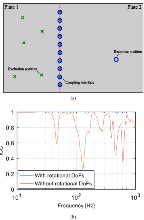
The interface completeness criterion (ICC) has been devel-oped to quantify the extent to which the chosen interface de-grees of freedom provide a true representation the physical sys-tem. The essential concept, illustrated in figure (2), is that a force on one side of the interface will produce zero response on the other side if the interface is fully blocked. Blocking of the interface is not feasible physically but it can be achieved math-ematically at the degrees of freedom included in the model, de-noted,ck, in figure (2). A non-zero response on the opposite
side from the excitation is then taken to indicate the presence of unaccounted interface degrees of freedom,cui.e. a lack of
The ICC is defined as follows [8]:
Cba =
Yba
ˆ Yba
H 2
Yba(Yba)HYˆba
ˆ Yba
H (3)
where Yba is the FRF with excitation at a and response at b
etc. (see below) and Yˆba = YbckY −1
ckckYcka. A complete in-terface corresponds toCba =1 and indicates that there are no
neglected paths, i.e.cu=0. At the other extreme,Cba=0
indi-cates a totally incomplete interface description, in other words that none of the interface paths are included in the model, so
ck=0.Cbahas previously been termed the Interface
[image:5.595.314.546.254.607.2]Complete-ness Criterion (ICC) for consistency of terminology with, for example the Frequency Response Assurance Criterion (FRAC) [9] although both are more accurately ‘coefficients’ rather than ‘criteria’.
Figure 2: Illustration of the interface completeness criterion (ICC) concept: the interface is (mathematically) blocked at the known degrees of freedom,ck; a
non-zero response atbon the receiver R due to excitation ataon the source S then indicates the presence of neglected degrees of freedom at the interface,cu,
i.e. a lack of completeness in the model of the interface.
The FRFs needed for evaluation of the ICC, as defined in equation (3) are: Ybci,Y
−1
cici andYcia. The ICC is equally valid for classical and blocked force TPA, however, since all FRFs required are measured with the source and receiver connected, then fewer additional measurements are required for blocked force TPA than for classical TPA:
1) Ybck contains the accelerances with response atband ex-citation on the interface atck. These would normally be
measured in blocked force TPA if at least some of the in-dicator positions are atb(on the receiver away from the interface);
2) Y−ck1ckcontains accelerances with response and excitation both on the interface atck. This would normally be
mea-sured in blocked force TPA if the indicator positions are atck(on the interface);
3) Ycka contains the accelerances with excitation at loca-tionsaon the source side of the interface and responses on the interface atck. This would not normally be
mea-sured, however, it is a fairly simple additional measure-ment since accelerometers will already be placed atckin
any case. This can be considered as a ‘artificial excita-tion’ of the source with the hammer.
An example of the ICC is given in figure (3) which indi-cates that the continuous interface between two halves of a plate is almost completely described by forces and moments at 10 discreet points on the interface (blue curve). However, when the moments are neglected the completeness is significantly re-duced over certain frequency ranges (orange curve).
(a)
[image:5.595.86.241.291.490.2](b)
Figure 3: Illustration of the Interface completeness criterion (ICC). Top: ‘plate 1’ and ‘plate 2’ are two sides of the same flat plate connected through a contin-uous interface. Contincontin-uous forces and moments along this interface are repre-sented by generalized forces at 10 discreet points (the ‘model’). Bottom: ICC with forces and moments included (blue); forces only (brown).
3.2. Consistency
systems. It was shown in [10, 11] that this can result in signif-icant errors in certain frequency ranges. This can be illustrated by expressing the measured operational acceleration in terms of the ‘true’ force (or blocked force), ftrue, and the true FRF
matrix,Ytrue.
a=Ytrueftrue (4)
Note that the acceleration is measured directly and we do not have access to the terms on the right hand side so the ‘true’ FRF matrix,Ytrue, is implied in the acceleration measurements but
is not obtained explicitly. When the inverse step is applied, as in equation (1), we pre-multiply by the inverse of the measured FRF matrix,Y:
f=Y+(Ytrueftrue) (5)
Clearly, if there is consistency between the ‘true’ FRF matrix,Ytrue,
and the measured one,Y, then the FRF matrices in equation (5) cancel and the estimated forces (or blocked forces)fare equal to the true values. However, if there is any inconsistency then the cancellation will be incomplete. A typical scenario is when there is a shift in the frequency of a resonance or antiresonance, perhaps due to temperature or load changes; around the peak or trough, the FRF changes rapidly and a small shift in frequency can result in significant artefacts over a narrow frequency range due to lack of cancellation. Note that incompleteness in the model, as described above, is one possible cause of inconsis-tency. Ideally, it will be possible to quantify the consistency through a metric similar to the ICC developed above. However, this problem will be addressed in a later paper.
4. Propagation of measurement uncertainties
The aim of the uncertainty analysis outlined in this section is to quantify the uncertainties inherent in the estimates of the target quantity,p. In this section, we consider those uncertain-ties originating in the various TPA experiments (experimental uncertainty); we also consider source uncertainty since this may readily be evaluated as part of the same general approach. We start with a general framework for measurement uncertainties which is then applied to TPA. We go on to describe how the necessary inputs are obtained in the measurement phases and provide relationships for propagating the measured uncertain-ties through to the target quantity.
4.1. Framework for measurement uncertainties
Consider a general input-output system described by:
y=Ax (6)
wherexis ann×1 vector of inputs,yanm×1 vector of outputs andAis them×nsystem matrix. The problem is to propagate the uncertainties inherent in the quantities on the right hand side through to the outputs on the left hand side.
For uncertain inputs,x, the covariance between any two el-ements of the output can be expressed using the law of error propagation as:
Σy=JxΣxJTx (7)
whereΣyis the covariance matrix of the output andΣxthe
co-variance matrix of the input. For real inputs,Σxis of dimension n×n, but since the inputs in TPA will generally be complex this becomes 2n×2n, since the real and imaginary parts must be described separately (as described later). Similarly,Σyis of
dimension 2m×2m.Jxis the Jacobian which is defined in terms
of the derivatives of equation (6) with respect to each input and is of dimension (for complex inputs) 2m×2n. In the following it will be described how to calculate the Jacobian from measured quantities. Further details about the derivation can be found in [7].
If, as well as the inputs,x, the system matrix,A, is also un-certain then additional terms are required to express the output covariance:
Σy=JxΣxJxT+JAΣAJTA (8)
whereΣAis the covariance matrix for the uncertain system
ma-trix which, for a complex mama-trix, has dimension 2mn×2mn.JA
is the Jacobian formed from the derivatives of equation (6) with respect to the elements of the system matrix and is of dimension 2m×2mn.
Equation (8) assumes no correlation between the inputs and the system matrix which is a fair assumption for TPA since the operational and FRF tests are performed at different times. De-spite this simplification, it is evident from equation (8) that a large number of elements are required to account for all possi-ble cross correlations, particularly those between the elements of the system matrix. It is tempting to introduce further sim-plifying assumptions at this point, for example, the covariance matrixΣAof the system matrix is diagonal if there is no
correla-tion between the elements [12]. However, when using hammer measurements, it is usual to measure a full column of the ma-trix simultaneously in which case the elements within a column will be correlated to some extent. It has been shown that these correlations can have a significant influence on the output vari-ances so the temptation to simplify will be resisted and all terms will be retained in the following analysis [12].
4.2. General framework applied to TPA
Having identified the general approach in the previous sus-bsection, we now proceed to apply this to the TPA problem. In effect, we apply the law of error propagation outlined in equa-tion (8) to the forward and inverse steps of the TPA process as defined in equations (2) and (1) respectively.
4.2.1. Forward (prediction) step
Starting with the forward (prediction) step given in equation (2), it is noted that this is of the same form as equation (6). The law of error propagation defined in equation (8) can therefore be applied directly to give the covariance matrix of the target response (cabin sound pressure):
Σp=JfΣfJfT+JHΣHJTH (9)
where Σf is the covariance matrix of the forces (or blocked
forces for blocked force TPA) andΣHthe covariance matrix for
the measured FRF matrixH. Jf andJHare the corresponding
Symbol Description How obtained
Σa
Covariance matrix of measured operational indicator responses
Calculated from re-peated measurement of operational response vectora
ΣH
Covariance matrix of measured FRF matrix,
H
Calculated from re-peated measurement of FRF matrixH
ΣY
Covariance matrix of measured FRF matrix,
Y
Calculated from re-peated measurement of FRF matrixY
Jf
Jacobian relating to
force vector,f See equation (24) JH
Jacobian relating to
FRF matrix,H See equation (26) Ja
Jacobian relating to
re-sponse vector,a See equation (27)
JY
Jacobian relating to FRF matrix,Y
[image:7.595.351.557.572.650.2]See equation (28) for square matrices and (29) for non-square matrices
Table 1: Quantities required for the calculation of measurement uncertainty in TPA.
The covariance matrix Σp of the target responses are the
quantities sought from this analysis. On the right hand side we have two covariance matrices, Σf, ΣH and two Jacobians, Jf
andJH, which need to be evaluated before we can obtain this
desired quantity. Of these,ΣHcan be obtained from measured
FRFs as described in [7, 13] and in the following. The Jaco-bians can also be described in terms of directly measured quan-tities as given in [13] and described later. The forces however are not measured directly and so an additional step is required to obtain their covariance matrix,Σf, as described in the
follow-ing.
4.2.2. Inverse (force identification) step
Equation (1) shows that the forces (or blocked forces),f, are not measured directly but are inferred from other measured quantities in the inverse step of TPA. Applying the law of error propagation, equation (8), to equation (1) we obtain:
Σf =JaΣaJTa +JY+ΣY+JTY+ (10)
whereΣais the covariance matrix of the indicator responses,a.
In effect, these are the ‘source’ uncertainties. Ja is the
corre-sponding Jacobian.ΣY+is the covariance matrix for the pseudo
inverse of the measured FRF matrixY+andJY+the
correspond-ing Jacobian.
Note that since the directly measured quantity is the FRF matrixYrather than its pseudo inverseY+, an additional step is required to propagate uncertainties of the measured FRFs through the matrix inversion. Fortunately, it is possible to rewrite equation (10) in a form more convenient for TPA as follows
[14]:
Σf =JaΣaJaT+JYΣYJTY (11)
whereΣYis the covariance matrix for the (directly measured)
FRF matrix, Y. JY is a correspondingly modified Jacobian
which will be given later and again, is calculable from mea-sured quantities. A derivation of equation (11) will be provided in [14]. Note that, whilst equation (8) provided an exact prop-agation of uncertainty (as equation (6) is linear), equation (11) provides only a first order approximation because the inverse of a matrix is non-linear function. The JacobianJYtherefore
pro-vides a first order relation betweenYandY+and equation (11) is valid only in the presence of ‘low levels’ of FRF uncertainty. Combining the results from this and the previous subsection we see that in order to calculate the desired variances of the target responsesΣp we require three covariance matrices and
four Jacobians as summarized in Table 2. How to obtain these quantities will be shown in the following. However, first we briefly consider the issue of complex data.
4.2.3. Handling of complex data
In frequency domain TPA, as discussed here, all quantities will generally be complex. We therefore must consider the vari-ance in both the real and the imaginary parts of each quantity and furthermore, the covariance between the real and imaginary parts. Therefore, in order to express the variance of a single complex quantity a 2×2 covariance matrix is required:
σxixj → " σ
<(xi)<(xj) σ<(xi)=(xj)
σ=(xi)<(xj) σ=(xi)=(xj) #
(12)
whereσxixj is the covariance between elements i and j of a
measured matrix or vector, and<( ) and=( ) represent real and imaginary parts respectively. For example, in the case ofi= j,σ<(xi)<(xi)is the variance of the real part,σ=(xi)=(xi)is that of
the imaginary part andσ<(xi)=(xi) =σ=(xi)<(xi)is the covariance
between real and imaginary parts.
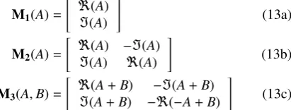
Fortunately, the required transformations can be handled relatively straightforwardly in the programming stage of analy-sis [10, 14, 15] by the use of three complex matrix operators as defined below:
M1(A)= "
<(A)
=(A)
#
(13a)
M2(A)= "
<(A) −=(A)
=(A) <(A)
#
(13b)
M3(A,B)= "
<(A+B) −=(A+B)
=(A+B) −<(−A+B)
#
(13c)
Each can be implemented in one line of code. For reference, the first,M1( ), applies to vectors, the second,M2( ), to
ana-lytic matrices satisfying the Cauchy Riemann equations and the third,M3( ), to complex matrices not satisfying the
ele-ments. The reader is referred to [10, 14, 15] for further infor-mation on derivation and application.
4.3. Obtaining the covariance matrices
We now consider how the required covariance matrices are obtained from measurements. We start with the indicator re-sponse vector,a, before going on to treat the FRF matrices,Y
andH. Again, we stress the importance of correct and consis-tent ordering of all elements of all matrices and vectors.
4.3.1. Covariance matrix of response vector,Σa
In effect, the covariance matrixΣarepresents the source
un-certainty, (although the measured values will to some extent be modified by the receiver structure to which the source is at-tached). To obtain the covariance matrix, the response vector,a
(assumedn×1), is measured multiple times, sayktimes in total. The resulting column vectors are arranged horizontally and the real part of each element is stacked on top of the corresponding imaginary part by elementwise application of theM1( )
oper-ator (see equation 13a). The resulting measurement matrix is of dimension 2n×k:
¯a=h M1(a(1)) M1(a(2)) · · · M1(a(k)) i
(14)
wherea(i)is the column vector of responses measured in theith
measurement. For clarification, the expanded form of equation (14) is given by:
¯a=
<(a1(1)) <(a1(2)) · · · <(a1(k))
=(a1(1)) =(a1(2)) · · · =(a1(k))
<(a2(1)) <(a2(2)) · · · <(a2(k))
..
. ... ... ...
=(an(1)) =(an(2)) · · · =(an(k))
(15)
The covariance matrix is then obtained from equation (14) in the conventional manner using:
Σa=
1
k h
(¯a−E(¯a)) (¯a−E(¯a))Ti (16)
where the expectationE( ) is taken along the rows.
4.3.2. Covariance matrix of FRF matrix,,ΣY
In the evaluation of the FRF covariance matrices two ad-ditional factors arise that were not present for response vector, namely the need for multiple measurements and for reorganiza-tion of the FRF data.
The first point is that the FRF matrix,Y, must be recorded multiple times in order for the statistics to be evaluated. Whilst as described above, this is common practice for response mea-surements, it is not usual for FRF measurements to be processed in this way. In fact, the data is usually available because multi-ple measurements of FRFs are generally taken, however the in-dividual results are typically discarded after averaging with no attempt to evaluate higher order statistics. However, by retain-ing the data from each measurement it is possible, as described below, to evaluate variance without resorting to any additional
measurements. In the case of hammer measurements, this sim-ply means that the results of each hit must be saved.
The second point is that, whereas FRF matrices are nor-mally arranged such that the rows and columns correspond to response and excitation positions, for calculation of variance we require the correlations between every pair of matrix elements and a more convenient pattern is to arrange all the FRF elements into a single column vector. This can be achieved using a ‘vec-torization’ operation, consisting of stacking the columns of the FRF matrix beneath each other moving left to right. This oper-ation is simple to perform in many programming languages.
Considering the above, it is then possible to construct a measurement matrix similar to that for the response measure-ments defined in equation (14):
¯
Y=h M1(vec(Y(1))) M1(vec(Y(2))) · · · M1(vec(Y(k))) i
(17) where, as with equation (14), the superscripts in brackets refer to the number of the measurement wherekis the total number of measurements made. vec( ) represents the vectorization operator as described above, thus,vec(Y(i)) represents the entire
FRF matrix for measurementiin vectorized form. M1( ) is
the complex operator as defined in equation (13a) which again is applied elementwise.
Noting the similar form of equation (14) and (17) we can then express the covariance matrix in the same form as equation (16):
ΣY=
1
k
¯
Y−E(Y¯) Y¯ −E(Y¯)T
(18)
where the expectationE( ) is taken along the rows.
4.3.3. Covariance matrix of FRF matrix,ΣH
The covariance matrix for the target location FRFs,H, can be treated in the same way as that for the indicator location FRFs,Y. It is simply necessary to replaceYwithHin equa-tions (17) and (18). The resulting equaequa-tions are given below for completeness:
¯
H=h M1(vec(H(1))) M1(vec(H(2))) · · · M1(vec(H(k))) i
(19) and
ΣH=
1
k
¯
H−E(H¯) H¯ −E(H¯)T
(20)
4.4. Evaluating the Jacobians
Having obtained the necessary covariance matrices from the previous section, the remaining quantities required from table 2 are the four JacobiansJa,Jf,JY,JH.
4.4.1. General forms of Jacobian
eren-tials of the outputs with respect to the uncertain inputs,
Jx=
∂y1
∂x1
∂y1
∂x2 · · ·
∂y1
∂xn
∂y2
∂x1
∂y2
∂x2 · · ·
∂y2
∂xn
..
. ... ... ...
∂ym
∂x1
∂ym
∂x2 · · ·
∂ym
∂xn (21)
For the simple example of equations (6) and (7) this results in
Jx=A.
If in addition to the input vector, the system matrix is uncer-tain, an additional term is needed as was introduced in equation (8). The corresponding Jacobian,JAis obtained by partial
dif-ferentiation of the outputs with respect to each of the uncertain matrix entries:
JA=
∂y1
∂A11
∂y1
∂A21 · · ·
∂y1
∂Amn
∂y2
∂A11
∂y2
∂A21 · · ·
∂y2
∂Amn
..
. ... ... ...
∂ym
∂A11
∂ym
∂A21 · · ·
∂ym
∂Amn (22)
This is a similar form to equation (21) except that the number of columns is increased to allow for partial differentiation by all
mnentries of the matrix. Thus, the dimension ofJAism×mn
and it containsmdiagonal matrices arranged horizontally, each containing a repeated element of the vectorx.
JA=
x1 0 0 x2 0 0 · · · xn 0 0
0 ... 0 0 ... 0 · · · 0 ... 0
0 0 x1 0 0 x2 · · · 0 0 xn
(23) =xT⊗I.
The compact form of notation on the righthand side introduces the Kronecker product, ⊗, where every term of the matrix or vector on the left of the symbol is multiplied by the matrix or vector on the right. Fortunately, the Kronecker product is a standard function in many programming languages which fa-cilitates implementation of the above.
4.4.2. Jacobians required for TPA
We now present expressions for the Jacobians required in TPA starting with those for the prediction step outlined in tion (2). We note that equation (2) is of the same form as equa-tion (6), so the Jacobian Jf from equation (9) can be written
as:
Jf =M2(H) (24)
where the complex matrix operatorM2( ) (equation (10b)) has
been introduced to deal separately with the real and imaginary parts. The second Jacobian from equation (9) is of a similar form to equation (23), so:
Jf =M2(fT⊗I) (25)
This can be rewritten in terms of directly measured quantities by substituting in equation (1), giving:
Jf =M2((Y+a)T⊗I) (26)
where, again, M2( ) has been applied to deal with real and
imaginary parts.
We now consider the inverse step outlined in equation (1), for which a similar analysis can be applied, albeit slightly com-plicated by the presence of the pseudo inverse. The first term of equation (11) is similar to that of equation (9) which leads to:
Ja =M2((Y+) (27)
The remaining Jacobian,JY, requires a more involved analysis
because of the pseudo inverse and the result is presented here without derivation; the reader is referred to [14] for further de-tails. For square matricesJYtakes the following form:
JY=M2((−Y−1a)T⊗Y−1) (28)
However, when the matrix is non-square, which will often be the case, a lengthier expression is needed using the third form of the complex matrix operator from equation (13c):
JY=M3((−Y−1a)T⊗Y−1),([((I−YY+)a)T⊗Y+Y+H]+· · ·
· · ·[(Y+Y+Ha)T⊗(I−YY+)]K) (29) whereKis known as a commutation matrix and gives a relation betweenKvec(A)=vec(AT) [16].Kis uniquely defined by the dimensions ofA. For example, ifAis of dimensions 3×2,K
is given by,
K=
1 0 0 0 0 0
0 0 0 1 0 0
0 1 0 0 0 0
0 0 0 0 1 0
0 0 1 0 0 0
0 0 0 0 0 1
(30)
All of the elements necessary for evaluation of the source and experimental uncertainties are now available. The procedure is summarized in the following.
4.5. Summary for source and experimental uncertainties
The procedure for calculating uncertainties can be summa-rized by substituting equation (11) into equation (9):
Σp=Jf(JaΣaJTa +JYΣYJTY)J T
f +JHΣHJTH (31)
The following steps are then required:
1) Σa is evaluated by repeated measurement of the
opera-tional response vector, a, and calculation of the covari-ance matrix according to equations (14, 16);
2) ΣYis evaluated by repeated measurement of the FRF
Figure 4: System for numerical example. The source and receiver are both flat plates. The red dot is the location of the ‘internal’ operating forces of the source (not normally accessible). The target response,p, is evaluated at the yellow dot and indicator responses,a, at the interface locations (green). The FRF matrix, Y(4×4), is evaluated at the interface locations (green) andH, (1×4) between the interface and target locations.
3) ΣYis evaluated in a similar fashion toYusing equations
(19, 20);
4) The JacobiansJa,Jf,JY,JH are evaluated using
equa-tions (24, 26, 27, 28);
5) Values for all terms are substituted into equation (31).
4.5.1. Correlation betweenYandH
Note that equation (27) and all the preceding analysis as-sumes there is no correlation between the indicator position FRFs, Y, and the target position FRFs, H. This is a reason-able assumption if they are obtained in separate tests, which would occur for reciprocal measurement for example with a volume velocity source. However, if forward FRF measurement is used, with structural excitation at the interface then it is pos-sible to obtain responses at both indicator and target locations simultaneously, in which case there will be correlation within the columns ofHandYand an additional term is required in equation (27):
Σp=Jf(JaΣaJTa+JYΣYJTY)J T
f +JHΣHJTH+2JHYΣHYJTHY (32)
Based on analysis in [13], the most likely effect of neglecting this correlation is a significant overestimation of the overall un-certainty. Since the estimates are likely to be on the safe side a full analysis of this effect will be left to a later paper. How-ever, it is worth mentioning that there are potentially important implications for whether forward or reciprocal measurement of FRFs provides the most reliable results in TPA.
5. Numerical Example
In this section, the estimation of uncertainties in TPA is il-lustrated by a numerical example. Measurement examples of certain aspects of the above analysis are also provided in [7, 13]. The system evaluated is shown in figure (4). The source and receiver are both flat plates, connected at the top of 4 rigid con-nections. The lack of repeatability in the hammer hits for the
FRF measurements is simulated by randomly varying the ex-citation position which leads to an ensemble of measurements with the spread shown in the upper plot of figure (5). The FRF covariance matrices,ΣY andΣHY are evaluated from this
[image:10.595.316.545.208.416.2]en-semble. The FRF variance has been selected for illustration purposes to lie on the high side of what would be expected from a typical physical measurement. The receiver response is contaminated by noise as shown in the lower plot of figure (5) leading to estimates of response variance,Σa.
Figure 5: Upper: example mean FRF with spread of results from different ham-mer hits. Lower: example receiver response showing the spread of results with added noise.
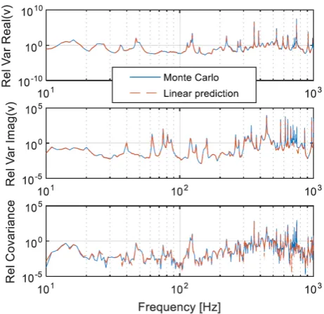
Figure 6: Bivariate uncertainty of the predicted response (compared against a Monte-Carlo solution)
[image:10.595.319.550.481.705.2]imag-inary parts of the target response as predicted from the above calculation scheme. Note that the covariance between the real and imaginary parts is significant and cannot be neglected. Also shown are the results from a Monte-Carlo analysis of the same data. Results indicate that the first order analysis described ear-lier provides a good estimate of uncertainties in the output, at least for the level of input uncertainty level considered (believed to be realistic).
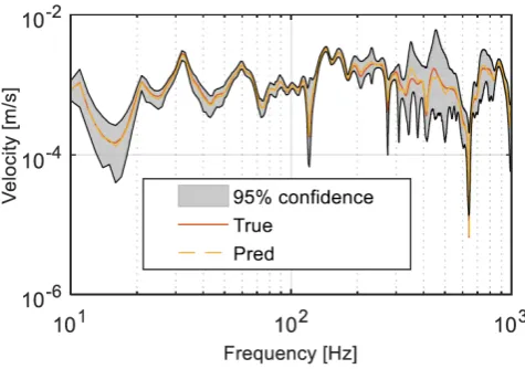
[image:11.595.45.283.320.487.2]Figure (7) shows the predicted magnitude of the target re-sponse overlaid with the 95% confidence intervals obtained from the above analysis. These confidence intervals were obtained assuming the real and imaginary parts of the response were joint normally distributed. A Monte-Carlo method was then used to estimate the confidence bounds for the magnitude of the re-sponse [13]. It can be seen that for this example the variance at low frequencies (¡50 Hz) primarily derives from background noise in the indicator responses. However, at high frequencies (300-600 Hz) the main source is the lack of repeatability in the FRF measurements.
Figure 7: Predicted magnitude of the target response with a 95% confidence bounds
6. Summary/Conclusions
The uncertainties affecting TPA measurements have been categorized as: model, source and experimental. Model uncer-tainties occur due to incompleteness or inconsistency in the rep-resentation of the physical system by the measurements and are a significant potential cause of error. The Interface Complete-ness Criterion (ICC) has been introduced as a way of quanti-fying the (lack of) completeness. A corresponding metric for consistency is under development.
Source and experimental uncertainties are random varia-tions. A first order framework for estimating the influence of these input uncertainties on the target quantity in both classi-cal and blocked force TPA has been outlined and illustrated by a numerical example. Three covariance matrices are required for the input quantities, i.e. the indicator accelerations and the FRFs for indicator and target locations. In addition, four Ja-cobian matrices are required which can all be calculated from directly measured quantities. No additional measurements are
required over and above the usual TPA measurements, although additional data storage and calculation is required.
References
[1] M.V. van der Seijs, D.D. Klerk, and D.J. Rixen. General framework for transfer path analysis: History, theory and classification of techniques.
Mechanical Systems and Signal Processing, pages 1–28, 2015. [2] J.W. Verheij. Multi-path sound transfer from resiliently mounted
ship-board machinery. PhD thesis, TNO, 1982.
[3] B J Dobson and E Rider. A review of the indirect calculation of excita-tion forces from measured structural response data. Proceedings of the Institution of Mechanical Engineers, Part C: Journal of Mechanical En-gineering Science 1989-1996 (vols 203-210), 204(23):69–75, 1990. [4] A. S. Elliott, A. T. Moorhouse, T. Huntley, and S. Tate. In-situ source
path contribution analysis of structure borne road noise.Journal of Sound and Vibration, 332(24):6276–6295, 2013.
[5] F.X. Magrans. Method of measuring transmission paths.Journal of Sound and Vibration, 74(3):321–330, 1981.
[6] A.T. Moorhouse, A.S. Elliott, and T.A. Evans. In situ measurement of the blocked force of structure-borne sound sources.Journal of Sound and Vibration, 325(4-5):679–685, sep 2009.
[7] J.W.R. Meggitt, A.S. Elliott, and A.T. Moorhouse. A covariance based framework for the propagation of uncertainty through inverse problems with an application to force identification.Mechanical Systems and Signal Processing, (124):275–297, 2019.
[8] J.W.R. Meggitt, A.T. Moorhouse, and A.S. Elliott. On the problem of de-scribing the coupling interface between sub-structures : an experimental test for ’completeness’. InIMAC XVIII, pages 1–11, Orlando, 2018. [9] R.J. Allemang. The Modal Assurance Criterion (MAC): Twenty Years of
Use and Abuse. InProceedings of SPIE - The International Society for Optical Engineering, volume 4753, pages 397–405, 2002.
[10] J.W.R. Meggitt, A.S. Elliott, A.T. Moorhouse, A. Clot, and R.S. Langley. Development of a Hybrid FE-SEA-Experimental Model: Experimental Subsystem Characterisation. InNOVEM: Noise and Vibration - Emerging Methods, Ibiza, 2018.
[11] A. Clot, R. S. Langley, J.W.R. Meggitt, A.T. Moorhouse, and A.S. Elliott. Development of a Hybrid FE-SEA-Experimental Model: Theoretical For-mulation. InNOVEM: Noise and Vibration - Emerging Methods, Ibiza, 2018.
[12] J.W.R. Meggitt. On the treatment of uncertainty in experimentally mea-sured frequency response functions.Metrologia, 55:806–818, 2018. [13] J.W.R. Meggitt and A.T. Moorhouse. A Combined Framework for the
Propagation of Uncertainty in Transfer Path Analysis.(In Preperation). [14] J.W.R. Meggitt, A.S. Elliott, A.T. Moorhouse, G. Banwell, H. Hopper,
and J. Lamb. Broadband characterisation of in-duct acoustic sources using an equivalent source approach.Journal of Sound and Vibration, 2018. [15] J.W.R. Meggitt and A.T. Moorhouse. A covariance based framework
for the propagation of correlated uncertainty in frequency based dynamic sub-structuring.Mechanical Systems and Signal Processing (Submitted), 2019.
[16] A. Hjorunges. Complex-Valued Matrix Derivatives. Cambridge Univer-sity Press, 1st edition, 2011.
Contact information
Prof Andy Moorhouse, Acoustics Research Centre, Univer-sity of Salford, Manchester, M5 4WT, UK.
Email: [email protected]
Acknowledgements
Definitions/Abbreviations TPA transfer path analysis
ICC interface completeness criterion, or
interface completeness coefficient