Determining Optimal Textural Features for Cervical Cancer lesions using the Gaussian Function

(1)

International Journal of Emerging Technology and Advanced Engineering

Website: www.ijetae.com (ISSN 2250-2459, ISO 9001:2008 Certified Journal, Volume 4, Issue 6, June 2014)

89 Determining Optimal Textural Features for Cervical Cancer

lesions using the Gaussian Function

S. Pradeep Kumar Kenny

1

, Dr. S. Allwin

2

1_{Centre for Information Technology & Engineering, Manonmaniam Sundaranar University, Tirunelveli} 2_{Dept. Of Computer Science and Engineering, Infant Jesus College of Engineering and Technology, Tuticorin, India.}

Abstract— Cervical cancer is one of the most deadliest gynaecologic cancer occurring in women and it is also a very important research area in image processing. The main reason as to why this cancer is so deadly is that it cannot be detected early as it doesn’t throw any symptoms until it evolves to the final stages of cancer. The reasons attributed to this is the cancer itself and also to the lack of pathologists available to screen the cancer especially in third world countries. One solution would be to automate the system. But this comes with a set of problems as we have a number of features to determine whether the given cell is cancerous or not. If we calculate with too many features then the accuracy goes up but speed comes down. And if you reduce the features it is the other way round. To strike a balance between the speed and accuracy of a system in this paper we have proposed a unique ranking system using Gaussian function to determine the right balance of features which can be used in an automated system.

Keywords— Cancer, Cervical cancer, Cervical cytology Gaussian function, Textural features

I. INTRODUCTION

Cervical cancer is now considered as the contributor of most number of deaths among women worldwide. It is curable if it is detected and treated in its initial stage. But detecting the cancer in its initial stage is difficult because it shows symptoms only in the later stages. The traditional screening methods available like the visual procedures take a long time and often produce incorrect results. Further it is highly impossible for a few pairs of eyes to screen each and every woman on the planet. To solve this problem an automated process is needed. An automated process could not only accelerate the process and but it also could give accurate results. Normally all automated systems consist of three phases [12] namely pre-processing phase for removing noise and image correction, segmentation phase to isolate the ROI form the rest of the image and feature extraction phase to extract the properties of the images using various mathematical formulas.

Image segmentation is an image analysis task wherein you individually decompose the various object present in an images. You can decompose the image into disjoint regions so that within each region the features will have strong, visual similarity, reasonable homogeneity and statistical correlation. Image segmentation algorithms are classified into different groups like region based techniques, feature thresholding, clustering techniques, contour based techniques, [1]-[11] etc.

All these approaches different advantages and limitations in terms of computational cost, performance, applicability and suitability.

Once segmentation is completed then the most important job is features extraction. In the real world we see a lot of things with our eyes. Although our eyes see the image it’s the brain that interprets that image. The brain describes each and every image using its shape, spatial location and textural properties. Color, brightness and contrast are all a subpart of textural properties. Using textural properties we can make out what a surface it really is. You can tell whether an object surface is rough, smooth, broken etc. A red ball and red apple from a distance can be distinguished by the texture of the object. Technically a texture is the measure of light refracted from the surface. A rough surface appears rough because half of the light bouncing out of the surface doesn’t bounce back the same way as the other half does. So if you take an old wooden plank then you see dark spots. It means the light which fell on that surface has bounced back the other way and hence your brain interrupts that as a rough surface.

There are plenty of mathematical formulas to determine these variances and that is the problem which is faced by an automated system. When you have too many features for detecting you are hard pressed as to which feature extraction technique needs to be used. If you use too much features it slows down the system and if you use too little then it brings down the accuracy. Hence a right balance has to be struck. Therefore the available features have to be ranked in some way so that we can have the right combination of features.

Nowadays with rise of new innovative computational methods there are plenty of ways to do this. In this paper we have proposed a novel ranking system by making use of Gaussian function. This paper has been organized into IV sections. Section II discusses how the features extracted and classified. And Section III shows the results. Conclusions are made in Section IV.

II. IMPLEMENTATION

(2)

International Journal of Emerging Technology and Advanced Engineering

[image:2.595.50.302.139.203.2]

90

Figure 1. Block Diagram

A. Input Image

We obtain the image of the cervix by extracting cells from the cervix using a swab and it is placed in a slide. This is then digitalised and the resulting image is obtained. A sample cervical image is shown Figure 2[12].

Figure 2. Cervical Cyto Image

B. Pre-Processing

The obtained image cannot be used directly as it presents a set of weak features. Also the region of interest which is the nucleolus needs to be separated from the rest of the image. There are numerous methods proposed for doing this [1]-[11].

[image:2.595.298.560.429.781.2]

The pre-processing technique employed in this paper converts the RGB image into Gray scale colour model and then filters the noise with the help of a median filter and process the image using a set of morphological operators to strengthen the image. At the end we end up getting an image as shown in figure 3 [12][13].

Figure 3 Segmented Image

Now that the ROI is separated from the rest of the image we can extract the features better.

C. Feature Extraction

There are several textural features available but in this paper the gray level co-occurrence matrix (GLCM) features, Haralick, gradient and tamura based features are taken for analysis.

GLCM is the simplest way of describing the features in an given image. It makes use of statistical moments present in the intensity moments of the intensity histogram of an image.





       



N z N y j y x I and i y x I if Otherwise y z

j

i

P

1 1 ) , ( ) , ( , 1 , 0

)

,

(

(1)

Where and are the image intensity values, and are the spatial positions in an image and the offset (Δz, Δy) specifies the distance between the pixel-of-interest and its neighbour.

In 1973 Haralick introduced 14 statistical features which are obtained by calculating the values for each one of the co-occurrence matrix obtained by averaging the four values using the directions 0o, 45 o, 90 o and 135 o. The Symbol Δ representing the distance parameter, can be selected as one or higher. In general Δ can be set to 1

as the distance parameter Where is the

extinction image after intensity conversion.

(2)

(3)

In Tamura features, in an Image we calculate a value for the three features at each pixel and treat these as a spatial joint coarseness-contrast-directionality (CND) distribution

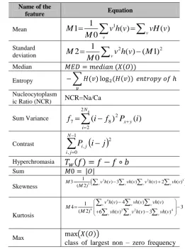
In this paper we have employed around 34 features for our analysis. The features implemented are listed in table I [14]-[18].

TABLEI

TEXTURAL FEATURE EXTRACTION

Name of the

feature Equation

Mean

1

( )

0

v

M

v h v

vH v

M









Standard deviation 2 2

1

2 ( ) (

1)

0

v

M

v h v

M







Median

Entropy ∑

Nucleocytoplasm

ic Ratio (NCR) NCR=Na/Ca

Sum Variance



 





Ng

i y x

i

P

f

i

f

2 2 2 8

7

(

)

(

)

Contrast







 



1 0 , 2 , N j i j i

i

j

P

Hyperchromasia

Sum | |

Skewness





3 2 3

3 1

3 ( ) 3 ( ) ( ) 2 ( )

( 2) v v v v

M v h v vh v v h v vh v M

     

Kurtosis

4

4 2 2 4

( ) 4 ( ) ( )

1

4 3

( 2) 6 ( ) ( ) 3 ( )

v v v

v h v vh v vh v M

M vh v v h v vh v

           



Max ( )

[image:2.595.128.209.504.573.2]

(3)

International Journal of Emerging Technology and Advanced Engineering

91

of h

Autocorrelation





i j

j

i

p

j

i

f

₆

(

,

)

(

,

)).

Correlation



 













_

1 0

, 2 2

,

)

)(

(

)

)(

(

N j

i _i _j

j i j i

j

i

P





Cluster Prominence













i j xy

x

p

i

j

i

f

₈



4

(

,

).

Cluster shade

f





_i _j



i



j



x



xy



p

(

i

,

j

).

3

7



Dissimilarity





i j

j

i

p

j

i

f

6

,

.

(

,

).

Energy





i j

j

i

p

f

₁

{

(

,

)}

2

Entropy of

GLCM







i j

j

i

p

j

i

p

f

₉

(

,

)

log

(

,

))

Homogeneity









i j

j

i

p

j

i

f

(

,

)

(

1

2 5 Maximum Probability

).

,

(

,

10

p

i

j

i

MAX

f



Sum of average



 



Ng i y x

i

iP

f

2 2

6

(

)

Sum of square

variance





_







        1 0 , 2 , 2 1 0 , 2 , 2 N j i i j i i N j i i j i

i P i   P j 



Sum of entropy

(

)

log

{

(

)}

2

8

P

i

P

i

f

_x _y

N i y x g   





Difference variance y x

p

f

₁₀



variance

of

_

Differnce Entropy



   





1 0

11

(

)

log

{

(

)}

g N i y x y

x

i

P

i

P

f

Information Measurement of Correlation 1& 2

}

,

{

1

12

HY

HX

MAX

HXY

f





2 1 13

(

1 exp

[

2 .

0 (

HXY

2 HXY

)])

f











i j

j

i

p

j

i

p

HXY

(

,

)

log

(

,

))

Where HX and HY are entropies of px and py, and



 

i j

y x i p j

p j i p

HXY1 (, )log( () ( ))



  i j y x y

x i p j p i p j

p

HXY2 () ( )log( () ( ))

Inverse

difference



_

_

2

,

1 i

j

C

_i_j

Inverse difference

normalized









G j i ij

G

j

i

C

1 , 2 2

/

1

Inverse difference moment

normalized













G j i ij

G

j

i

C

1 , 2 2

/

1

Coarseness Step 1:-

For every point calculate differences between the not overlapping neighborhoods on opposite sides of the point in horizontal and vertical direction:

| | | _|

Step 2:-

At each point select the size leading to the highest difference value:

Step 3:-

Finally take the average over 2S as a coarseness measure for the image:

(4)

International Journal of Emerging Technology and Advanced Engineering

92

Where

is the number of pixels in the cell nucleolus region

is the number of pixels in the cytoplasmic region f is the grayscale image

b is the structuring element is the opening operation

is the total number of elements in the ROI frequency of pixel value

is the total number of elements in the ROI is the mean

is the standard deviation

is the set of all pixels of X in O which is the class of largest non – zero frequency of h

is the entry in the normalized graytone spatial dependence matrix

and is the number of distinct gray levels in the quantized image.

and are the means and standard

deviations of and .

∑ ∑

and is the number of distinct gray levels in the quantized image.

is the Sum of Entropy features

and are entropies of and

∑ ∑ , ∑ ∑ be the _{entry in normalized GLCM.}

_∑

in which represents the number of

number of occurrences of gray levels I and j within the given window, given a certain pair (

-interpixel distance -orientation) and G is the quantized number of gray levels.

∑ ∑ is the fourth moment about the mean

is the variance of the gray values present in the image and has to be experimentally determined to

be .

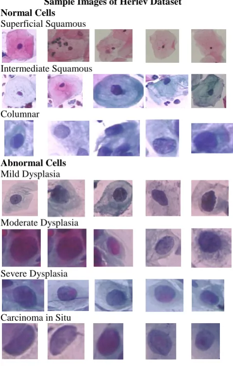
D. Herlev Dataset

In this paper we need to find a set of features that would work as a group to help find the better balance of features. The data set being used to test the hypothesis is the Herlev data set, which consists of 917 single pap smear images[19]. Cyto technicians and doctors have manually classified each cell into one of the 7 classes, namely superficial squamous, intermediate squamous, columnar, mild dysplasia, moderate dysplasia, severe dysplasia and carcinoma in situ. The first three correspond to normal classes and the last four classes correspond to abnormal classes as show in figure 4.

The pre-classification helps to serve as the gold standard for the entire work.

Sample Images of Herlev Dataset Normal Cells

Superficial Squamous

Intermediate Squamous

Columnar

Abnormal Cells

Mild Dysplasia

Moderate Dysplasia

Severe Dysplasia

[image:4.595.315.555.169.545.2]

Carcinoma in Situ

Figure 4. Sample images of the Herlev Dataset

E. Outlier Deletion

(5)

International Journal of Emerging Technology and Advanced Engineering

93

The test is based on the difference of mean and the most extreme data considering the standard deviatio given dataset with assumed normal distribution. The test is based on the following formulas [20]

(4)

(5)

Where

or =the suspected single outlier (max or min) =standard deviation of the whole data set

Once the outliers are deleted the total percentage of images present are calculated using the following formula

(6)

Where

is the total images present in a stage after deletion of outliers

is the total images present in a the given dataset for a particular stage

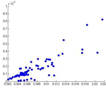
Using the above formulas we plot each and every feature value for each image of a particular feature of a particular stage. In Figure 5 a sample for the Nucleo cytoplasmic ratio feature for Superficial Squamous stage is shown. As you can see the the ones that do not work well for this feature are far away from the cluster and using this we can calculate the percentage of success for each feature for each stage.

F. Ranking

Once the features have been extracted and the outliers are deleted we are left with a percentage count. Now we can just do a normal rank and take the top 5 or you can take values above 90%. But doing so sacrifices the efficiency of the overall system. Hence a unique ranking system is proposed. The features in the database are listed after outlier detection as columns representing stages and rows representing features. Now as we mentioned above there may be many probable’s and to scrutinize this we use a Gaussian function. Using this function a bell curve is drawn over the values after segregating them into bins as shown in Figure 6. It is calculated using the following equation

[image:5.595.336.522.137.293.2]

( ) (7)

Figure 5. Nucleo cytoplasmic ratio feature for Superficial Squamous stage

Figure 6 A sample Bell Curve

Like in outlier detection the ones with less proximity fall to the bins located in the edges and the one with more prominence are in the middle. Using a manual upper and lower threshold we can segregate the values that would make it into the list. Here the threshold is 50%. But we can change this in ordinance to accuracy and speed needed for the automated system.

III.EXPERIMENTAL RESULTS

The above discussed methodologies where

[image:5.595.335.556.332.520.2]

(6)

International Journal of Emerging Technology and Advanced Engineering

94

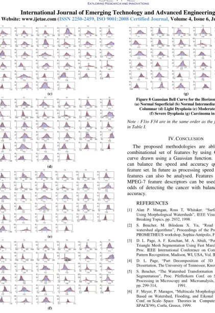
[image:6.595.310.554.135.447.2]

The features discussed in Table I are extracted and the outliers are determined and deleted and the percentage of success is calculated and is shown in table II. Then the values left after outlier deletion are taken and are segregated into bins and a bell curve is drawn over them. This is shown in figure 8. For each images the bell curve is drawn. These bins are so arranged that the ones with less proximity are clearly visible. By setting a maximum and minimum threshold values we can obtain the necessary values. Here in this work we are not mentioning the threshold value which has to be weighed between accuracy and speed. Unlike segmentation algorithms where threshold can be defined here it depends on factors like processing speed, need of the client. From the graph it is clear that the bins in the middle will be the high proximity values that can create a combinational set of features

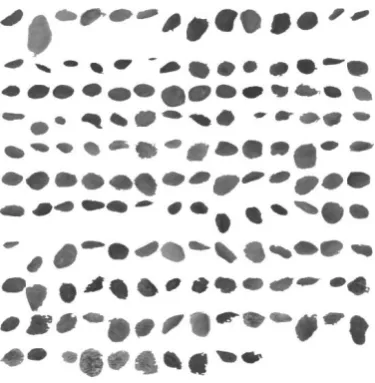
Figure 7. Carcinoma-in-situ image segmented

[image:6.595.71.259.333.525.2]

The percentage of values after removing outliers is shown in table II

TABLE III

Percentage of liable images after outlier deletion

F S1 S2 S3 S4 S5 S6 S7

1 90.54 75.71 84.69 86.26 82.88 88.83 74.67 2 82.43 78.57 84.69 73.08 87.67 81.73 78 3 85.14 84.29 83.67 85.71 81.51 86.8 83.33 4 74.32 74.29 79.59 78.02 77.4 88.83 83.33 5 81.08 72.86 87.76 90.66 84.25 84.77 84 6 81.08 72.86 81.63 89.01 83.56 87.82 83.33 7 79.73 72.86 74.49 87.91 74.66 83.25 79.33 8 83.78 72.86 87.76 84.62 87.67 82.74 91.33 9 81.08 87.14 89.8 88.46 78.77 79.7 84.67 10 87.84 50 84.69 53.3 87.67 85.79 93.33 11 72.97 88.57 96.94 74.18 85.62 82.23 82 12 85.14 81.43 81.63 84.07 85.62 87.82 97.33 13 89.19 80 77.55 91.21 87.67 77.16 92.67 14 90.54 92.86 87.76 79.67 88.36 90.36 85.33 15 87.84 84.29 82.65 89.56 83.56 71.07 74.67

16 91.89 92.86 80.61 82.42 87.67 86.8 86.67 17 90.54 92.86 87.76 79.67 88.36 90.36 85.33 18 72.97 77.14 85.71 78.02 85.62 79.19 82 19 85.14 84.29 80.61 89.01 74.66 80.71 85.33 20 86.49 87.14 80.61 86.81 85.62 82.74 78 21 85.14 82.86 79.59 86.26 78.77 77.66 72 22 72.97 91.43 83.67 80.22 89.73 86.29 80 23 81.08 94.29 83.67 71.98 87.67 82.74 81.33 24 91.89 94.29 80.61 82.42 82.19 85.79 80.67 25 75.68 82.86 80.61 66.48 89.73 79.7 86.67 26 90.54 90 83.67 85.71 79.45 77.66 84.67 27 71.62 85.71 85.71 87.36 87.67 77.16 75.33 28 85.14 87.14 80.61 81.32 82.19 83.25 78.67 29 83.78 87.14 75.51 90.11 75.34 81.22 77.33 30 77.03 82.86 87.76 88.46 82.19 86.8 90 31 79.73 77.14 89.8 59.34 78.77 80.71 85.33 32 87.84 90 79.59 75.27 84.93 76.14 80.67 33 72.97 81.43 88.65 78.02 84.25 88.32 92 34 74.32 71.43 82.65 78.57 83.56 84.77 85.33 Where

Abnormal Cells Normal Cells

S1: Carcinoma in Situ

S5: Columnar

S2: Mild Dysplasia

S6: Intermediate Squamous

S3: Moderate Dysplasia

S7: Superficial Squamous

S4: Severe Dysplasia

F Features

Note: The order of the stages has been changed to help in computation.

Features 1 to 34 represent the same order as in Table I

(a)

[image:6.595.42.287.594.775.2]

(7)

International Journal of Emerging Technology and Advanced Engineering

95

(c)

(d)

(e)

(f)

[image:7.595.66.488.88.701.2]

(g)

Figure 8 Gaussian Bell Curve for the Horizontal Ranking (a) Normal Superficial (b) Normal Intermediate (c) Normal

Columnar (d) Light Dysplasia (e) Moderate Dysplasia (f) Severe Dysplasia (g) Carcinoma in Situ

Note : F1to F34 are in the same order as the features ordered in Table I.

IV.CONCLUSION

The proposed methodologies are able to create a combinational set of features by using Gaussian bells curve drawn using a Gaussian function. Using this we can balance the speed and accuracy quotient of the feature set. In future as processing speed increase other features can also be analysed. Features like wavelets, MPEG-7 feature descriptors can be used to better the odds of detecting the cancer with balanced speed and accuracy.

REFERENCES

[1] Alan P. Mangan, Ross T, Whitaker. ―Surface Segmentation Using Morphological Watersheds‖, IEEE Visualization '98: Late Breaking Topics, pp. 2932, 1998.

[2] S. Beucher, M. Bilodeau X. Yu, ―Road segmentation by watershed algorithms‖, Proceedings of the Pro-art vision group PROMETHEUS workshop, Sophia-Antipolis, France, 1990. [3] D. L. Page, A. F. Koschan, M. A. Abidi, ―Perception-based 3D

Triangle Mesh Segmentation Using Fast Marching Watersheds‖, Proc. IEEE International Conference on Computer Vision and Pattern Recognition, Madison, WI, USA, Vol. II, pp. 27-32, 2003. [4] D. L. Page, ―Part Decomposition of 3D Surfaces‖, Ph.D.

Dissertation, The University of Tennessee, Knoxville, 2003. [5] S. Beucher, ―The Watershed Transformation Applied to Image

Segmentation‖, Proc. Pfefferkorn Conf. on Signal and Image Processing in Microscopy and Microanalysis, Cambridge, UK, pp. 299-314, 1991.

(8)

International Journal of Emerging Technology and Advanced Engineering

96

[7] F. Meyer, S. Beucher, ―Morphological Segmentation‖, Journal of Visual Communication and Image Representation, 1(1):21-45, 1990.

[8] R. Lotufo,W. Silva, ―Minimal set of markers for the watershed transform‖, Proc. ISMM, 2002.

[9] R.Gonzalez, R.woods: ―Digital Image Processing‖. Addison Wesley, 1993.

[10] Susanta Mukhopadhyay and Bhabatosh Chanda. ―Multiscale Morphological Segmentation of Gray Scale Image‖ IEEE Transactions on Image Processing, Vol.12, No. 5, May 2003. [11] A.K.Jain: "Fundamentals of Digital Image Processing",

Englewood cliffs.N: Prentice - Hall 1989.

[12] S.Allwin, S.Pradeep Kumar Kenny*, V.Manian, ―Classification of stages of maligancies using textron signatures of a cervical cyto image‖, Computational Intelligence and Computing Research (ICCIC),IEEE, 978-1-4244-5965-0, pp 1-4, Dec 2010.

[13] Krishnan Nallaperumal, Krishnaveni. K, et.al ―An efficient Multiscale Morphological Watershed Segmentation using Gradient and Marker extraction‖,INDICON, 2006.

[14] Rodenacker K, Bengtsson E., "A feature set for cytometry on digitized microscopic images", Anal Cell Pathol, pp 1-36, 2003 [15] Fritz Albregston., Statistical Textural Measures Computer from

Gray Level Coocurrence Matrces. 2008

[16] Prof. Dr.-Ing.H.Ney., Features for Image retrieval, December 2003

[17] R. M. Haralick, K. Shanmugam, I. Dinstein, ―Texture features for image classification.‖ IEEE Trans. System Man Cybernat, 8 (6), 1973, pp. 610-621.