LANGUAGE MODEL FOR DIGITAL RECOURSE OBJECTS RETRIEVAL

3077

INCREMENTAL PARALLEL CLASSIFIER FOR BIG DATA

WITH CASE STUDY: NAÏVE BAYES USING MAPREDUCE

PATTERNS

1_{VERONICA S. MOERTINI,} 2_{MOHAMAD F. SEPTRIANTO,} 3_{LIPTIA VENICA} Informatics Department, Parahyangan Catholic University, Bandung, Indonesia 1_{[email protected],} 2_{[email protected],} 3_{[email protected]}

ABSTRACT

Classification methods can be used to derive values from big data in the form of models, which then can be utilized to predict new cases. Several parallel classification methods for big data have been developed based on Hadoop MapReduce as well as for Spark system. As big data keeps on coming, the models must be updated from time to time to represent the old as well as the new data. The computations must be efficient and scalable for handling big data.

This research aims to enhance the existing parallel classifiers such that they will perform as incremental classifier handling batches of big data. The research results are presented as follows. First, the architecture and main concept of the enhancement is presented. Secondly, the proposed incremental parallel Naïve Bayes classifier (NBC) based on MapReduce that handles dataset with discrete attributes is discussed in detailed. Two series of experiment were performed on Hadoop clusters with 5 and 10 nodes. The results show that the incremental parallel NBC has acceptable accuracy, is efficient and scalable.

Keywords: big data classification method, incremental parallel classifier, MapReduce patterns

1. INTRODUCTION

Big data is volume, velocity, and/or high-variety information assets that demand cost-effective, innovative forms of information processing that enable enhanced insight and decision making [1]. It comes in structured, semi-structured and unstructured format. Processing big data requires new, innovative, and scalable technology to collect, host and analytically process the vast amount of data gathered in order to derive values. These values may relate to profit, medical or social benefits, or customer, employee, or personal satisfaction.

Classification methods can be used to derive values from big data in the form of models, which can be utilized to predict new cases. The required big data sometimes must be gathered from several sources and comes with different formats. This leads to complexity in preparing the needed data such that it can be fed into classification algorithms. The activities may involve advanced technologies, processes and algorithms. As big data along with other non-big data keeps on coming, the models must be “updated” from time to time to “represent”

the current data. To renew the model, batches of preprocessed big data can be produced periodically then fed into the selected classification algorithms. In this regard, incremental classifiers that work based on batches of preprocessed big data are needed.

3078 Apache Spark with its RDD (Resilient Distributed Datasets), which can run on top of Hadoop’s YARN resource manager, has been developed to address the MapReduce weakness [6,7]. Machine Learning algorithms that require iterative computations can be implemented on Spark. As in standalone implementation, the algorithms can then access the data from memory (stored as RDD objects), which is a lot faster than reading from disks. A Spark library of machine learning algorithms (MLLib), which has clustering (such as k-Means) and classification (Naïve Bayes, SVM and RandomForest) functions, have been developed and can be adopted.

Although incremental parallel classifiers that work based on batches of big data are needed, based on our literature study results (see Subsection 3.1 and 3.2), we have not found any technique based on Hadoop MapReduce and Spark that specifically address this problem. Therefore, this research objective is to develop or enhance the existing parallel classifiers that have been developed for Hadoop or Spark environment such that they will perform as incremental classifier handling batches of big data. The classifier must have approximately the same accuracy (compared to the existing classifier) and must be efficient and scallable. Having this objective, in this research:

(1) We reviewed groups of classification methods and identify which groups are suitable to be enhanced. (The group includes as Bayesian, decision tree, lazy learning, rule based and neural network [8].

(2) We studied research results related to those classification methods that have been enhanced or implemented for Hadoop and Spark, then analyzed the potencies of enhancement.

(3) Based on the above results, we designed the overall system architecture and the main concept of enhancement.

(4) From (2), we found that Naïve Bayes classifier (NBC) handling discrete attributes of dataset can be enhanced to handle batches of big data efficiently by adopting MapReduce summarization and meta patterns. It involves only one pass computation and read the training dataset once. Thus, we designed the detailed enhancement (as a case study) and conduct two series of experiments to evaluate the performance.

This paper presents our research results and is organized as follows: Literature review of basic concept (bagging, NBC, Hadoop and MapReduce patterns, Apache Spark, the evaluation of parallel classifiers and the main concept of enhancement, proposed parallel classifier architecture system,

detailed discussion of proposed incremental parallel NBC, two series of experiment for evaluating the NBC performance conducted on a Hadoop cluster, conclusion and further works.

2. LITERATURE REVIEW

2.1. Bagging: Ensemble Classifier Methods

Classification is a two-step process. First, a model is built from a training dataset. Secondly, the model is evaluated using test data set. If the model’s accuracy is acceptable, the model is later used to classify new data. Depending on the “nature” of the dataset and the selected classification algorithms, the model accuracy is sometimes below the expectation. Bagging is a method used in ensemble methods to improve classification accuracy. An ensemble for classification is a composite model, made up of a combination of classifiers. The individual classifiers vote, and a class label prediction is returned by the ensemble based on the collection of votes. Ensembles tend to be more accurate than their component classifiers [8].

Baggingworks as follows (see Figure 1): D is a set of d tuples. For iteration i (i = 1, 2, . . . , k), a training set, Di , of d tuples is sampled with

replacement from the original set of tuples, D. (Because sampling with replacement is used, some of the original tuples of D may not be included in Di , whereas others may occur more than once.) A classifier model, Mi, is learned for each training set, Di. To classify an unknown tuple, X, each classifier, Mi, returns its class prediction, which counts as one

vote. The bagged classifier, M*, counts the votes and assigns the class with the most votes to X.

Internal Sources

D1

D2

Dk

M1

M2

Mk

Combine votes New tupple

Class predicted .

.

3079 2.2. Naïve Bayes Classifier

Naïve Bayes classifier (NBC) is a classifier, where the features of the vectors (representing tupples) are assumed to be conditionally independent of each other [8]. Given a vector X = (x1, x2, . . . . , xn), using

Bayes’ theorem, the conditional probability of X having a class value of Ck can be written as:

𝑃 𝐶 |𝐗 _𝐗𝐗| (1)

Because the features of X is assumed to be conditionally independent of each other, Eq. 1 can be rewritten as:

𝑃 𝐗|𝐶 𝑃 𝑥 |𝐶 𝑃 𝑥 |𝐶 . . . 𝑃 𝑥 |𝐶 (2)

In Eq. 2, if xi is discrete then P(xi|Ck) is simply the

number of tuples of class Ck having the value xi(for

attribute Ai ) divided by the number of class Ck. If xi

is continuous-valued then P(xi|Ck) is computed using

Gaussian distribution, by first computing mean and standard deviation of the attributes. The highest value of P(X|Ck) is selected and Ck is the predicted

class.

NBC model can be materialized as specific structure containing all of the pre-computed measures used in Eq. 2, which is used to predict the class of the new tupple. The measures include the Gaussian distribution for numerical attribute and count of each class values (for computing P(Ck)) and count of each

attribute values for each class value (for computing P(Ck|X)).

2.3. Hadoop, HaLoop and MapReduce Patterns

Hadoop, a platform for storing and analyzing big data in distributed systems, comes with master-slave architecture [2,3]. It has components of Hadoop Distributed File System (HDFS) and MapReduce. Its storage and computational capabilities scale with the addition of slave nodes to a Hadoop cluster, and can reach volume sizes in the petabytes on clusters with thousands of hosts. A brief overview of HDFS and MapReduce is as follows.

HDFS: It is a distributed file system designed for large-scale distributed data processing under frameworks such as MapReduce and is optimized for high throughput. It automatically re-replicates data blocks on nodes (the default is 3 replications).

MapReduce: It is a data processing model that has the advantage of easy scaling of data processing over multiple computing nodes. Map and Reduce functions run in each slave node in parallel. A

MapReduce program processes data by manipulating key-value pairs in the general form: map: (k1,v1) ➞ list(k2,v2)

reduce: (k2, list(v2)) ➞ list(k3,v3).

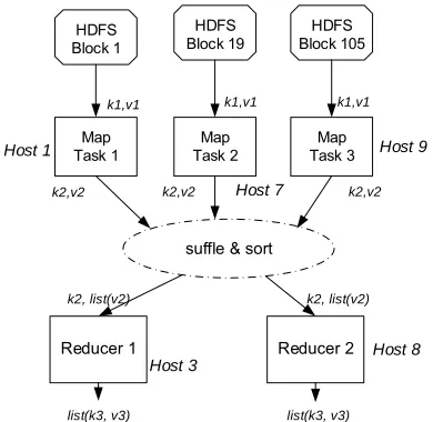
Map reads (key, value) pairs, then based on the algorithm designed by developers, it generates one or more output pairs list (k2, v2). Through a complex shuffle and sort phase, the output pairs are partitioned and then transferred to Reducer: Pairs with the same key are grouped together as (k2, list(v2)) and then each partition with unique value of k2 is sent to a Reducer. The Reduce function (with a specific algorithm assigned) generates the final output pairs list(k3, v3) for each group (see Figure 2).

A client submits a MapReduce job to the master, which then assign and manage Map and Reduce job parts to slave nodes. Map reads and processes blocks of files stored locally in the slave node, sent list of key-value to Reduce via shuffle and sort, then Reduce may write its computation results to HDFS.

Map

Task 1 Task 2Map Task 3Map

Host 1

Host 7

Host 9

HDFS Block 1

HDFS Block 19

HDFS Block 105

k1,v1 k1,v1 k1,v1

Reducer 1 Reducer 2

Host 3

Host 8

k2,v2 k2,v2 k2,v2

suffle & sort

k2, list(v2) k2, list(v2)

list(k3, v3) list(k3, v3)

Figure 2: Map, shuffle and sort, and reduce phases.

3080 To address that Hadoop disadvantage, HaLoop is

currently developed (see

https://code.google.com/archive/p/haloop/).

HaLoop not only extends MapReduce with programming support for iterative applications, but also improves their efficiency by making the task scheduler loop-aware and by adding various caching mechanisms. In short, HaLoop has the following features: (1) Provide caching options for loop-invariant data access, (2) let users reuse major building blocks from applications' Hadoop implementations, and (3) have similar intra-job fault-tolerance mechanisms to Hadoop. HaLoop is backward-compatible with Hadoop jobs. However, currently, HaLoop is only a prototype system and has not been released a production system.

MapReduce Design Pattern

MapReduce design pattern is a template for solving a common and general data manipulation problem with MapReduce. It is not specific to a domain such as text processing or graph analysis, but it is a general approach to solving a problem intended to build better software [5]. As MapReduce is a relatively new technology with a fast adoption rate and there are new developers joining the community every day, the design patterns also provide a common language for teams working together on MapReduce problems. There are several MapReduce design patterns that have been designed, such as summarization, filtering, data organization, join, input and output and meta patterns. Below is the excerpt of patterns that are adopted in our proposed technique, which are summarization and meta patterns.

Summarization Pattern

Data can be large and “vast”, with more data coming into the system every day. This pattern aims to produce a top-level, summarized view of the data such that ones can glean insights not available from looking at a localized set of records alone. Summarization analytics are all about grouping similar data together and then performing an operation such as calculating a statistic, building an index, or just simply counting. The summarization patterns include numerical summarizations, inverted index, and counting with counters. They are more straightforward applications of MapReduce than some of the other patterns because grouping data together by a key is the core function of the MapReduce paradigm: All of the keys are grouped together and collected in the reducers. If the value fields emitted by the mapper is the ones intended to

be grouped by the key, the grouping is all handled by the MapReduce framework for “free”.

Numerical Summarizations: The numerical

summarizations pattern is a general pattern for calculating aggregate statistical values over the data. The intention of this pattern is to group records together by a key field and calculate a numerical aggregate per group to get a top-level view of the larger data set. The summarization function, θ, is executed over some list of values (v1, v2, v3, …, vn) to

find a value λ, i.e. λ = θ(v1, v2, v3, …, vn). Examples

of θ are counting, minimum, maximum, average, median, and standard deviation. Numerical summarizations should be used when both of the following are true: The data is numerical or countable and can be grouped by specific fields. This pattern is generally used in word count, record count,

finding min/max/count and

average/median/standard deviation.

The numerical summarization generally has three components as follows:

(a) The mapper outputs keys that consist of each field to group by, and values consisting of any pertinent numerical items.

(b) The combiner can greatly reduce the number of intermediate key/value pairs to be sent across the network to the reducers for some numerical summarization functions. If the function θ is an associative and commutative operation, it can be used for this purpose.

(c) The reducer receives a set of numerical values (v1, v2, v3, …, vn) associated with a group-by key

records to perform the function λ = θ(v1, v2, v3, …, vn). The value of λ is output with the given input key.

Meta Pattern

Many big data computing problems can not be solved using a single Map-Reduce job. Some jobs in a chain will run in parallel, some will have their output fed into other jobs, and so on. Job chaining pattern pieces together several patterns to solve complex and multistage problems. Job merging is an optimization for performing several analytics in the same MapReduce job.

3081 with the driver is the simplest method, where a master driver simply fires off multiple job-specific drivers. Here, the driver for each MapReduce job is run in the sequence as defined. The output path of the first job is the input path of the second. The first job must be checked for success before executing the second job.

2.4. Apache Spark

Spark is a general-purpose data processing engine, an API-powered toolkit which data scientists and application developers incorporate into their applications to rapidly query, analyze and transform data at scale [6, 7]. It is often used alongside Hadoop’s data storage module, HDFS, but can also integrate equally well with other popular data storage subsystems such as HBase, Cassandra, MapR-DB, MongoDB and Amazon’s S3. Spark’s flexibility makes it well-suited to tackling a range of use cases, and it is capable of handling several petabytes of data at a time, distributed across a cluster of thousands of cooperating physical or virtual servers. Typical use cases include stream processing, data integration, interactive analytics and analyzing data using machine learning techniques. Spark’s ability to store data in memory and rapidly run repeated queries makes it well-suited to training machine learning algorithms. It significantly reduces the time required to iterate through a set of possible solutions in order to find the most efficient algorithms.

Spark will normally run on an existing big data cluster. These clusters are often also used for Hadoop jobs, and Hadoop’s YARN resource manager will generally be used to manage that Hadoop cluster (including Spark). When Spark runs on top of Hadoop, it benefits from Hadoop’s cluster manager (YARN) and underlying storage (HDFS, HBase, etc.).

Spark Driver

Cluster Master Mesos, YARN or Standalone

Cluster Worker

Executor

Cluster Worker

Executor

Cluster Worker

Executor

Figure 3: Spark architecture [7].

Spark employs master slave architecture with one centralized coordinator, which is driver and with

many workers (Figure 3). At a high level, every Spark application consists of a driver program that launches various parallel operations on a cluster. The driver program contains the application’s main function and defines distributed datasets on the cluster, then applies operations to them. (The driver program can be the Spark shell, which takes operations from users.) Driver programs access Spark through a SparkContext object, which represents a connection to a computing cluster. Once a SparkContext object is created, it can be used to build Resilient Distributed Datasets (RDDs). Users can then run various operations accessing the RDDs. To run the operations, driver program typically manage a number of nodes called executors. For example, if the count() operation is run on a cluster aiming for counting file lines, different machines might count lines in different ranges of the file.

Resilient Distributed Datasets (RDDs)

The RDD is a concept at the heart of Spark. It is designed to support in-memory data storage, distributed across a cluster (as partitions stored in nodes) in a manner that is demonstrably both fault-tolerant and efficient. Fault-tolerance is achieved, in part, by tracking the lineage of transformations applied to coarse-grained sets of data. Efficiency is achieved through parallelization of processing across multiple nodes in the cluster, and minimization of data replication between those nodes. Having RDD, Spark supports efficient iterative computations, where each cycle needs to read large data, as the data is stored in parallel memory. Many machine learning or data mining algorithms, such as clustering, classification, association analysis involve iterative computations, thus are suitable to be enhanced for Spark environment.

A Spark library, namely Scalable Machine Learning on Spark (MLLib), has been available. It implements algorithms of classification, clustering, and so on. The classification algorithms are logistic regression, linear support vector machine (SVM), and multinomial and Bernoulli Naive Bayes, which are typically used for document classification.

3. PARALLEL CLASSIFIERS AND CONCEPT OF ENHANCEMENT

3082 The later stores all of the training tuples in pattern space and wait until presented with a test tuple before performing generalization (usually, lazy learners require efficient indexing techniques). Decision tree classifiers, Bayesian classifiers, classification by back propagation, support vector machines, and classification based on frequent patterns are all examples of eager learners. Nearest-neighbor classifiers and case-based reasoning classifiers are lazy learners.

If lazy learning is used to predict a class of a new case from big data, which can be petabytes in size, the computation will evaluate millions or even billions of records. This will be inefficient. Therefore, we conclude that lazy learners are not good candidates for classifying big data. Hence, we intend to find the classifier(s) that can be enhanced for classifying big data stream from the eager learner group based on Hadoop MapReduce as well as Spark.

3.1. Classification Methods Based on MapReduce

We found that few eager learner classifiers have been enhanced based on Hadoop MapReduce to handle big data. Aiming to enhance them into incremental classifier, below is our review of parallel decision tree classifiers, Bayesian classifiers, classification by back propagation, support vector machines, and classification based on frequent patterns:

(1) Decision tree: Decision tree induction is a top-down recursive tree induction algorithm, which uses an attribute selection measure to select the attribute tested for each non-leaf node in the tree. ID3, C4.5, and CART are examples of such algorithms using different attribute selection measures. In inducing a tree from the dataset, it adopts divide and conquer strategy in that the whole dataset is partitioned recursively. Early decision tree algorithms typically assume that the dataset are memory resident.

[9] proposes a parallel decision tree based on MapReduce via Sampling Splitting points with Estimation.

(2) Naïve Bayes: [10] and [11] have developed techniques to parallelize the NBC based on Hadoop MapReduce. From the results of experiment conducted in a Hadoop cluster with 4 machines (1 master and 3 slaves), [11] concludes that the executing time increases approximately linear with

the size of dataset and the size of data that can be processed is much larger than the standalone algorithms can handled.

(3) Backpropagation: Backpropagation is a neural network algorithm for classification that employs a method of gradient descent. It searches for a set of weights that can model the data so as to minimize the mean-squared distance between the network’s class prediction and the actual class label of data tuples. Rules may be extracted from trained neural networks to help improve the interpretability of the learned network. In computing the weights of the network model, the whole dataset must be fed as many as the epoch (iteration).

[12] have developed parallel backpropagation neural network (BPNN) based on MapReduce. The training data are bootstrapped (partitioned randomly) into samples, each is then fed into BPNN running in every client machine. In the training phase, the ensemble techniques including bootstrapping and majority voting have been employed.

(4) Support Vector Machine (SVM): A support

3083 The objective of this research is to develop efficient incremental classification method, suitable for batches of big data. Table 1 (located at the end of this article) presents the summary of the mapper and reducer tasks and the job.

3.2. Classification Methods for Spark

Unlike the ones designed based on MapReduce, the related research results of classifications methods for Spark that we found are basically the application of MLLib functions (Naïve Bayes, Logistic Regression, SVM and Random Forest). The excerpts are as follows:

(1) Parallel Naïve Bayes (NB) and Logistic Regression (LR) algorithms are used to classify large scale of Arabic Text [15]. Large-scale Arabic text corpuses are collected, followed by performing the proper text preprocessing tasks (sequential text preprocessing and term weighting with TF-IDF in parallel). Parallelized NB and LR algorithms are used to classify the texts in the Apache Spark environment. The experiment results indicate that both NB and LR gives high accuracy (89% and 93%), but NB was faster.

(2) Experiment using Ensemble Support Vector Machine (SVM) was performed using big data with the size of 3T, namely, Splice-Site [16]. The experiment results prove that Spark provides a high feature throughput on cached data, and that models trained in Spark reaches as good accuracy as algorithms trained in any other framework.

(3) [17] proposes Incremental Parallel Random Forest (IPRF) algorithm for data streams in Spark environment. IPRF basically optimizes the data allocation by designing RDDs that are distributed on the worker (slave) nodes and task scheduling for dynamic parallel optimization (but, the method is not clearly discussed). The decision trees are built using IPRF on the dynamic independent feature variables stored as RDDs in the worker nodes. The experiments were conducted using Solar Power System which consists 1,88,835 instances. Unfortunately, the experiments results are not clearly discussed. One result that can be concluded is that the the larger the streaming data size, the larger the error rate.

Thus, from the Spark classifier literature study it is found that: Large as well as stream dataset are handled well by parallel Naïve Bayes, SVM and Random Forest. The algorithms also reach good accuracy.

3.3. The Main Concept of Enhancement

The parallel classification techniques based on MapReduce and for Spark discussed in Subsection 2.3.1 and 2.3.2 can be enhanced into incremental classifier to handle batches of big data. The following is the general idea:

3.3.1 Using Ensemble Methods

Basically, all of the parallel classification methods [11, 12, 13, 14, 15, 16, 17] can be enhanced towards incremental ones using ensemble methods with bagging (see Figure 1). A batch of dataset:

(a) Can be split into one training data partition and test data. One additional model is constructed from the training data and added to the bag of models.

(b) Can be split into several training data partitions (similar to bootstrapping in [12]) and test data. Many models are constructed from these partitions and added to the bag of models.

On both approaches, the test data along with the old ones is then used to test the final bag of model. (It is also possible that the new test data only that is used to test the model. However, experiments are required to make sure that the model quality can be tested using that data only.)

Depending on the algorithms, the model can be a collection of statistic measures (for parallel Naïve Bayes), decision tree (for decision tree and RandomForest), NN model, SVM model or frequent pattern tree.

Issues and general idea of model constructions with MapReduce:

(a) The existing version of MapReduce does not support efficient iterative computation where each cycle reads the whole or part of dataset. Thus, the algorithms must be designed in such a way so that its number of iterations is as little as possible. Depending on the characteristic of the data input, this could be hard to achieve.

(b) Each Reduce function produces its own output (in this case, it can be “part of the model”). So, the algorithm design should include combining the Reduce outputs, if the job employed more that one reducer.

(c) Meta pattern can be adopted accordingly if the algorithm needs more that one pair of MapReduce functions.

3084 Issues and general idea of model construction: (a) Although RDD provides parallel in-memory dataset that can be read by Spark application many times, each task running in a worker will “see” and access its local RDD (the RDD objects stored in the node memory) only. Proper data structure and parallel algorithms must be designed to address this issue. If the task running on every worker is designed to compute “some part of the model”, there should be a mechanism to collect and combine all of the worker computation results properly.

(b) To address the above issue, one node can be designed to store one ore more local RDD that represents ensemble methods’ data partition (which must be randomized). Then, the task is designed to create some part of the global model from those local RDDs. With this regard, each worker produces one (or more) local model (that later will be collected into bag of models).

(c) Spark provides mechanism of collecting RDDs from all workers into the master node. The global model collected (or combined) must be fit into a single machine memory.

(d) The Spark application may access HDFS, so the application can be designed to read multiple batches of data stored in an HDFS folder.

Materializing the general idea discussed above will need lots and tedious research activities.

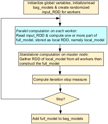
Initianlize global variables, initialize/read bag_models & create randomized

input_RDD for workers

Paralel computation on each worker:

Read input_RDD & compute one or more part of full_model, stored as local RDD, namely local_model

Standalone computation on master node:

Gather RDD of local_model from all workers then construct the full_model

Compute iteration stop measure

Stop?

Add full_model to bag_models

Figure 4: Core algorithm of computing bags of model on Spark.

3.3.2 Using Single Model

It is also possible to enhance parallel incremental classifiers that create a single model with non-degraded quality or accuracy. However, unlike with

ensemble methods, among of the methods discussed in Subsection 2.3.1 and 2.3.2, only one method can be enhanced. That is the parallel Naïve Bayes [11, 15] that handles dataset with discrete attributes only (which means, if there are numerical attributes, they must be transformed into discrete ones first). The model can be designed as the summarization (count) of the class and attribute values for each class value. When there is batch of data coming in, the new count is computed. The result is then used to update the previous (old) model (see Figure 5). Using MapReduce patterns, the method can be implemented efficiently as it involve a single pass computation only.

As the computation is simple, in this research this is the method that is designed (in detailed), implemented and evaluated through two series of experiments.

1 parallel

train

batch_model 2 update

model

final_model data batch

Figure 5: Steps of computing single model.

4. PARALLEL INCREMENTAL CLASSIFIER SYSTEM ARCHITECTURE

Preparing big data for classification, which may originated from many sources with various forms (structured, semi-structured or unstructured), involves complex processes. Those are data extraction and collection, combining or merging, selection, cleaning and transformation. To accomplish those tasks, few tools and complex computations may needed. Generating features from this data (for classification) would also involve complex computations.

Given these facts, we view that incremental parallel classifiers should handle batch of (preprocessed) data.

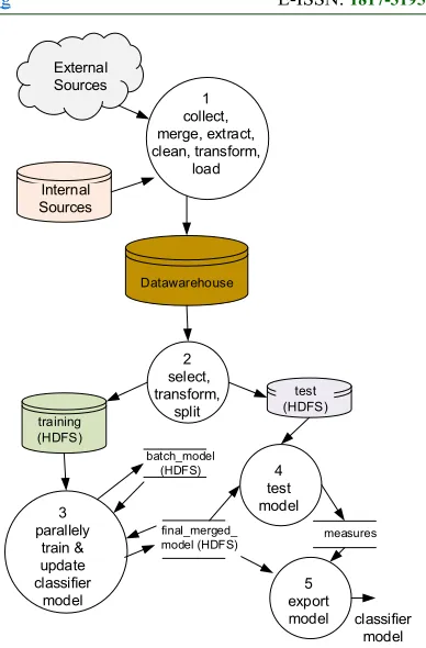
Our proposed general incremental classification system architecture that handle batches of big data is shown on Figure 6 and described as follows:

3085 data is then stored in a data warehouse (along with other various data).

(2) Based on the classification objectives, batch of big data of interest is prepared, which involve selection, merging, and other kind of transformation (for preparing the features). The batch can be split, large part (70-90%) is for training and the rest is for testing the model. The testing dataset is accumulated in a certain location (directory) in the HDFS (some of the old datasets can be erased after largely accumulated, if necessary).

(3) The training data is used to compute the temporary (batch) model, which is then “merged” with the existing model. After it is merged, the temporary model is erased (so is the training dataset, if intended to save space).

(4) The final-merged-model can be tested using the testing dataset and then the measures resulted (confusion matrix, accuracy, precision, recall and f-measure) are saved.

(5) If by evaluating the measures, the model passes the defined minimum values, the model can be exported and used in other systems for classifying new cases.

On the architecture presented on Figure 6, the algorithm adopted in Proses 3 (to create and/or update the model) can be the one that produces a single as well as bags of model. It is expected that the size of the model is a lot smaller than the training as well as testing dataset such that it can be exported to non-big data systems and be used in operational systems as needed.

Process 3 and 4 can be implemented in Hadoop (with MapReduce) or Spark. As discussed in the previous section, however, Hadoop currently does not support efficient iterative computation. So, for iterative algorithms, Spark with its RDD is a better option. For non iterative algorithms, MapReduce patterns can be adopted to support efficient computation.

External Sources

Internal Sources

1 collect, merge, extract, clean, transform,

load

Datawarehouse

2 select, transform,

split

test (HDFS) training

(HDFS)

4 test model final_merged_ model (HDFS) batch_model

(HDFS)

3 parallely

train & update classifier

model

5 export

model classifier model measures

Figure 6: The proposed architecture of incremental classification system for batches of big data.

5. INCREMENTAL NBC BASED-ON MAPREDUCE

In our previous works [18, 19], we found that the most contributing factor that degrades the MapReduce job performance is its repetitive HDFS files reading (by the mapper). It costs lots of IO processes. On the other hand, parallel NBC that handles discrete attributes only has advantages (Subsection 3.3.2): The job is run only once and the computation for updating or merging the model is simple. Numerical attributes can also be transformed into discrete attributes using histogram analysis or other techniques. Based on these reasons, we adopt NBC as a case in materializing Process 3 and 4 of Figure 6 that creates single model.

NBC Model Structure

To support simple access and computations by Map and Reduce functions, the NBC model is designed to include:

(1) The count of every class value with the structure: {class, value| CLASS – count}.

3086 atr2, val2, . . . atrn, valn| class, value | DISCR - count}.

‘DISCR’ is included to indicate that the attributes are discrete (to distinguish with CONT for enhancement in the future).

Example of part of a model: Play, No| CLASS – 7 Play, Yes| CLASS – 5

Outlook, sunny, Temperature, hot, Humidity, high, Wind, weak| Play, no| DISCR – 2

Outlook, overcast, Temperature, med, Humidity, med, Wind, weak| Play, yes| DISCR - 4

By using the above structures:

(1) The Reduce functions (in the training and updating model process) can be designed to directly emit outputs with the structures.

(2) The Map function (in the updating model process) can read each of the two structures as a record.

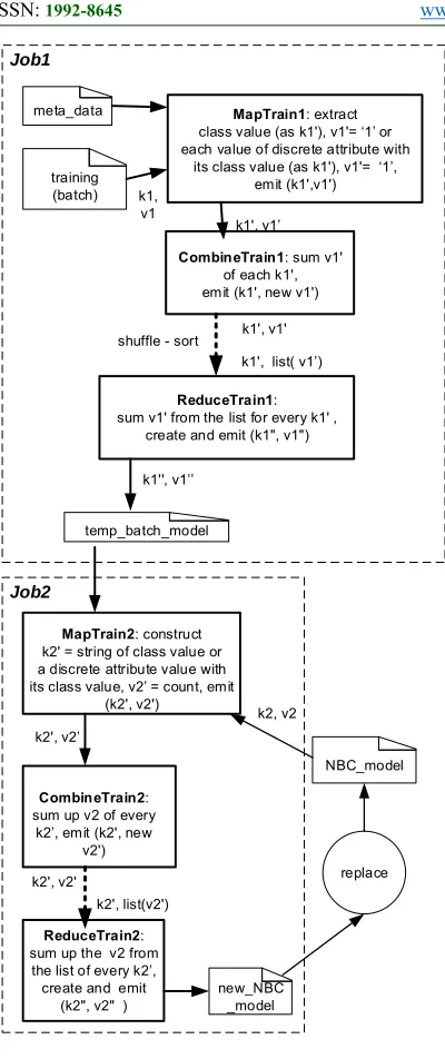
Module of Training and Updating the Model This module consists of two jobs, which are job for producing a model from the batch of data and updating the old model using the newly created model. To “connect” these 2 jobs, Job Chaining pattern [5] is adopted. Two MapReduce jobs are designed (see Figure 7): The first performs model construction from the batch of training data, which outputs the temporary model. The second job merges the existing (old) model with the temporary model. The results of merging then replaces the old model.

As the designed NBC model contains counts of class and predictor attribute values, the numerical summarizations pattern discussed in Subsection 2.3. is adopted. In the training, the function of θ performs group counting over:

(1) an attribute value of (v1), where v1 is class

attribute and

(2) list of values (v1, v2, v3, …, vn), where vi is

predictor or class attribute.

During updating the model, the function of θ sums up the count of old and batch model for the same value of (v1) and (v1, v2, v3, …, vn).

The adoption of MapReduce pattern on the incremental NBC training (Figure 7) is as follows: (1) Job Chaining pattern is implemented with driver: Job1 includes MapTrain1, CombineTrain1

and ReduceTrain1, and Job2 has MapTrain2,

CombineTrain2 and ReduceTrain2.

(2) The summarization pattern with counting function is materialized in Job1 (in MapTrain1,

CombineTrain1, and ReduceTrain1) and Job2 (in

MapTrain2, CombineTrain2, and ReduceTrain2).

The overall NBC incremental training involves three stages of process, which are:

(1) Job1: Read the incoming batch of training data and using the defined meta data, then compute the temporary NBC model. The model created

(temp_batch_model) is then moved to the HDFS

folder (/final_model) that store the existing model (namely, NBC_model).

(2) Job2: Read newly created temporary and the old (existing) NBC model from /final_model folder and “merge” them into a new model. This job can only be executed after Job1 is completed.

(3) Replace the old model with the new one.

3087 meta_data

training (batch)

MapTrain1: extract class value (as k1'), v1'= ‘1’ or each value of discrete attribute with

its class value (as k1'), v1'= ‘1’, emit (k1',v1')

temp_batch_model k1,

v1 Job1

ReduceTrain1: sum v1' from the list for every k1' ,

create and emit (k1", v1")

k1'', v1’’

CombineTrain1: sum v1' of each k1', emit (k1', new v1')

k1', v1’

k1', v1'

k1', list( v1’) shuffle - sort

MapTrain2: construct k2' = string of class value or a discrete attribute value with its class value, v2’ = count, emit

(k2', v2')

NBC_model k2, v2

Job2

new_NBC _model

replace

CombineTrain2: sum up v2 of every

k2’, emit (k2', new v2') k2', v2’

ReduceTrain2: sum up the v2 from the list of every k2’, create and emit

(k2", v2" ) k2', v2'

k2', list(v2')

Figure 7: Incremental NBC training using two MapReduce jobs.

The tasks of Map, Combine and Reduce function of Job1 and Job2 are presented in Figure 7. As MapReduce functions work on the basis of pair key-value input-output, designing the proper structure (content) of key-value is important. The Map and Reduce tasks and the structures of key (k) and value (v) are described below.

Job1: Computing the batch model

MapTrain1 function: See Figure 7 for its tasks.

Input:

meta_data: Describes the training data attributes and classes with the following structure:

meta_data = class attribute + column number of class attribute + {attribute_name, type, index of column number of attribute} + count of attributes Example:

@class :Play,4

@attribute :Outlook,0,DISCR;

Temperature,1,DISCR; Humidity,2,DISCR; Wind,2,DISCR

@Count :5

(The attribute type is includes, because Map is designed to reject any tupple/record that has non-discrete attribute.)

training: The incoming batch training dataset with

the following structure:

training = {attribute value} + class value Example:

rain, cool, normal, strong, no overcast, cool, normal, strong, yes overcast, cool, normal, weak, yes rain, mild, high, strong, no sunny, hot, high, weak, no Pair of k1-v1:

k1 = offset of the record (line) being read v1 = record of training. Example: sunny, hot, high, weak, no

Output:

k1’ = class|{attribute, value} + class v1’ = count of k1’

Example of pair of k1’-v1’: |_class|Play, no - 5

|Outlook,sunny, Temperature, hot, Humidity, high, Wind, weak| Play, no - 1

CombineTrain1 function: See Figure 7 for its tasks.

Input: the same with the output of MapTrain1. Output: k1’= k1, v1’ = count of k1’

Example pair of k1’-v1’: sunny, hot, high, weak, no - 2

ReduceTrain1 function: See Figure 7 for its tasks.

Input:

k1’ = class value|{attribute, value} + class value list(v1’) = {count}

Example pair of k1’-list(v1’): |_class|Play,no - [2,2,1]

|Outlook,sunny, Temperature, hot, Humidity, high, Wind, weak| Play, no - [1, 1, 3]

Output:

3088 k2” = class, class value, count | CLASS or |{attribute, value} + class + class value + count | DISCRETE

Example of pair k2”-v2”: Play,No,5.0|CLASS - null

Outlook,sunny, Temperature, hot, Humidity, high, Wind, weak| Play, no, 3| DISCR - null

Before Job2 is started, the file temp_batch_model is moved to the HDFS directory where NBC_model is stored.

Job2: Merging the batch and old models.

MapTrain2 function:

Input:

NBC_model and temp_batch_model have the

same structure content, which is the same with k2” of ReduceTrain1. Asboth files are located in one “logical” HDFS folder, the blocks created from the files spread across the cluster data nodes are treated as the “same” input by Map function. This function reads all of the local blocks sequentially.

Pair of k1-v1:

k1 = offset of the record (line) being read v1 = line of NBC_model or temp_batch_model

Example of v1: Play,No,5.0|CLASS

Outlook,sunny, Temperature, hot, Humidity, high, Wind, weak| Play, no, 3| DISCR

Output:

k1’ = class + class value + “CLASS” or {attribute, value} + class + class value + “DISCR”

v1’ = count of k1’ Example: pair of k1’-v1’

Play,No| CLASS - 5

Outlook,sunny, Temperature, hot, Humidity, high, Wind, weak| Play, no| DISCR - 3

Steps of the function:

Read a string of line from the input split and store it in v1

Parse v1

If v1 contains strings of the class attribute and its value only:

k1’ = class + class value + “CLASS” and v1’ = count of k1’

else // v1 contains predictor, class attributes //and their count

k1’ = {attribute, value} + class + class value

+ “DISCR” and v1’ = count of k1’ Emit(k1’, v1’)

CombineTrain2 function:

Input: the same with the output of MapTrain2. Output:

k1’ = k1, v1’ = count of k1’ Example pair of k1’-v1’:

Play,No| CLASS - 7

Outlook,sunny, Temperature, hot, Humidity, high, Wind, weak| Play, no| DISCR - 4

Steps of the function: For every k1’

Sum v1’ from all pairs of k1’-v1’ having the same value of k1’ and store it as new_v1’ Emit(k1’, new_v1’)

ReduceTrain2 function:

Input: Pair of k1’- list(v1’), where:

k1’ = class + class value + “CLASS” or {attribute, value} + class + class value + “DISCR”

list(v1’) = {count of k1’} Example pair of k1’-list(v1’):

Play,No| CLASS – [7, 2, 4] Outlook,sunny, Temperature, hot,

Humidity, high, Wind, weak| Play, no| DISCR – [4, 6, 8]

Output: The output format is the same with the output format of ReduceTrain1 as they both write the same model to HDFS files. The output itself is written to a HDFS file. Here, only k2” is defined (v2” is set with null):

k2” = class, class value, count | CLASS or {attribute, value} + class + class value + count | DISCR

Example of pair k2”-v2”: Play,No,12|CLASS - null

Outlook,sunny, Temperature, hot, Humidity, high, Wind, weak| Play, no, 17| DISCR - null

Steps of the function: For every k1’

Sum v1’ from all pairs of k1’-v1’ having the same value of k1’ and store it as count_v1’

If k1’ contains strings of the class attribute and its value only:

Create k2” = class, class value, count_v1 | CLASS

else

3089 class value + count_v1 | DISCR

Emit(k2”, null)

Module of Testing

The testing module consist only one MapReduce job (see Figure 8). The Map read the meta data, NBC model and testing dataset to compute confusion matrix, accuracy, precision, recall and F-measure. The Hadoop Map capable of reading multiple files from a certain HDFS directory. Hence, the testing dataset or files can be accumulated into an HDFS folder by the process that collects, preprocesses and splits the dataset.

The functions of MapTest and ReduceTest are described as follows.

meta_data

NBC model

MapTest: predit class value of every new case in test dataset, k' = class, v’ = information of prediction

results, emit (k’,v’) test

ReduceTest: compute confusion matrix, accuracy, f-measure, precision, recall for each class value, create

k” = class and confusion matrix, v” =other measures, emit(k”, v”)

measures k’', v’’

k', v’

k', list( v’)

Figure 8: Testing with one MapReduce job.

MapTest function:

The main task of this function is to predict the class value of a new case (read from test dataset). The files of meta_data and NBC_model are read by setup method to create objects of:

ClassContainer object that stores class values and

ClassSplitConf that stores its location/index,

name and type (must be discrete).

PredictorContainer object that stores all of predictor attributes and count, and AttrSplitConf that stores its location/index, name and type.

The test file is read line by line by map() method as k-v pair, the attribute values are used to predict the class value, while the actual class is also kept. The following is the description of k-v and k’-v’. Input:

k = offset of the record (line) being read v = record of test dataset. Example: sunny,

hot, high, weak, no

Output:

k’ = class attribute

v’ = predicted class value + probability + actual class value

Example of pair of k’-v’:

Play- predicted=Yes| prob=0.67.5| actual=Yes

Play - predicted=Yes| prob=0.51.1| actual=No

Play - predicted=No| prob=0.96.32| actual=No

By receiving (k,v), the map function reads

NBC_model and computes the every probability of v

being in every class value (using Equation 2 as presented in Subsection 2.2). The map then selects the class value that has the highest probability and emit the predicted class, probability and the actual class as pair of k’-v’ as shown above.

ReduceTestfunction:

The main task of this reducer is to compute measures, which are confusion matrix, accuracy, precision and recall, that are used to evaluate the performance of the NBC model (see Appendix A for discussion of these measures). Since all of the measures must be computed from all of the test instances (cases), to simplify the algorithm, a single reducer processes all of the k’-v’ dispatched by all mappers (in other words, in the job configuration, number of Reducer is set to 1). This reducer implements the formulas depicted in Appendix A. The input and output are described below.

Input:

k’ = class attribute list(v’) = {v’}

Example of pair of k’ - list(v’): Play {

predicted=Yes|pct=67.5%|actual=Yes, predicted=Yes|pct=51.1%|actual=No, predicted=No|pct=96.32%|actual=No, }

3090 The k” and v” are simply designed for grouping the output and easy writing to the output file. The k” and v” are described as follows:

k" = class attribute + confusion matrix

v” = accuracy + {class value, precision, recall} + F-measure

Example of k”: @Play

|No |Yes| | No | 3 | 1 | |Yes | 1 | 2 | Example of v”:

Accuracy = 0.71

Play = No, Precision = 0.67, Recall = 0.75, F-Measure = 0.7

Play = Yes, Precision = 0.75, Recall = 0.67, F-Measure = 0.7

Note: With this scheme, the job has the disadvantage in that all of v’ must fit into a machine memory that run the Reduce task. Hence, the selected node must have sufficient memory.

6. EXPERIMENTS

Two series of experiments were performed with the following purposes:

Experiments-1: Proving that the proposed incremental parallel NBC compute and generate models correctly and have accuracy with the non-incremental NBC. Batches of dataset were created from three small to medium real datasets then fed to the classifier. The model that created incrementally using batches will be compared with the model built once using the whole dataset using the test output measures.

Experiments-2: Proving that the proposed incremental parallel NBC is scalable and executed efficiently in processing big data in the Hadoop cluster.

Experiments-1:

The experiments were performed on a single node, with CPU of Intel i7-3770 operating at 3.4 GHz, 16 Gb of memory, and running Hadoop 2.7.1. There are three datasets used, which are edible and non-edible fungi, nurses recruitment, and US homicide crime record by FBI, discussed as follows:

(a) Using fungi dataset:

This small dataset contains records of many kinds of fungi and its classification (edible or poisonous). It is obtained from https://archive.ics.uci.edu/ ml/datasets/Mushroom. It contains descriptions of hypothetical samples corresponding to 23 species of gilled mushrooms in the Agaricus and Lepiota Family. Each species is identified as definitely edible, definitely poisonous, or of unknown edibility and not recommended. This latter class was combined with the poisonous one. The dataset size is 373.7 kb and contains 8,124 records. There are 23 discrete attributes, where 22 as predictors and 1 as class. The class values are edible (51.8%) and poisonous (48.2%). The predictor attributes are fungi’s properties, such as cap (its shape, surface, color), bruises, odor, gill, stalk, veil, ring, spore, population and habitat.

Methods of experiments: First, the whole data is split 80% (as training) and 20% (as testing). After the model is created with the training, it is then tested using the test dataset. For experimenting with batches, we divide the whole dataset into 2 parts (as batches). Each part is further split into training dataset (80%) and testing (20%). Hence, we have 2 pairs of dataset to build and test the NBC model. Each pair is then fed into the NBC classifier to build and test the incremental model. When testing the model, the previous test dataset is also included, hence the test dataset is accumulated. The results is depicted on Table 2 (see at the end of the article).

From the results presented in Table 2, it is shown that:

(1) The model constructed using the full dataset is equal or the same with the model resulting from merging of Batch-1 and Batch -2 models in terms of its size and quality (accuracy, precision, recall, F-measure).

(2) The MapReduce job for merging the existing and newly created model takes longer time to execute compared to the training job.

(b) Using nurses recruitment dataset:

3091 enrollment to these schools in Ljubljana, Slovenia, and the rejected applications frequently needed an objective explanation. The final decision depended on three sub problems: occupation of parents and child's nursery, family structure and financial standing, and social and health picture of the family. The dataset size is 1.1 Mb with12,962 records. It has 9 discrete attributes, where 8 attributes are the predictors and 1 attribute is the class. Predictor attributes are parents, has_nurs, form, children, housing, finance, social, health. The class attribut: accepted, where the values are very_recom, recommend, priority, spec_prior, not_recom.

Methods of experiments: It is analogous to the previous experiment with fungi dataset. However, in these experiments, the whole dataset into 4 parts (as batches). The results are depicted on Table 3 (see at the end of the article).

From the results presented in Table 3, it is shown that:

(1) The model constructed using the full dataset is equal or the same with the model resulting from merging of Batch -1, -2, -3 and -4 models in terms of its size and accuracy.

(2) The MapReduce job for merging the existing and newly created model takes longer time to execute compared to the training job.

(c) Using homicide dataset:

The data contains records of homicide collected by FBI from 1980 to 2014, obtain from https://www.kaggle.com/murderaccountability/hom icide-reports (downloaded on 29 April 2017). The size is 118.8 Mb with 638,654 records. Every record contains information of time, crime location, perpetrator and victim profile (such as gender, age, race, ethnicity), weapon, relationship between the perpetrator and victim, and count of perpetrator and victim. It has 24 attributes of numerical and discrete type. In this experiment, only the 10 discrete attributes which are relevant for predicting new cases are selected, which are:

Predictor attributes: crime_type, victim_sex, victim_race, victim_ethnic, perpetrator_sex, perpetrator_race, perpetrator_ethnic, relation, and weapon.

Class attribute: crime_solved, which has value of (solved or unsolved).

By selecting those 10 attributes, the size of the dataset becomes 56 Mb.

Methods of experiments: It is analogous to the previous experiment with fungi dataset. However, in these experiments, the whole dataset into 5 parts (as batches). The results are depicted on Table 4 (see at the end of the article).

From the results presented in Table 4, it is shown that:

(1) The model number of records and their size may be increased from a batch to the next batch, but the final model is the same with the one constructed with the full dataset.

(2) The model constructed from the full dataset is equal or the same with the model resulting from merging of Batch-1, -2, -3, -4 and -5 models in terms of its size and quality measure (accuracy, precision, recall and F-measure).

(3) In processing small size of batches, the MapReduce job for merging the existing and newly created model takes longer time compared to the training job.

Experiments-2:

The aims of the experiments are to measure the execution time of training (Job1) and merging models (Job2) using batches of data with different number of discrete attributes on a Hadoop cluster. Four sets of synthetic data batch having 5, 10, 15 and 20 attributes were generated. Each set consists of 10 batches and each batch contains 50.000.000 records with size of 550 Mb (for 5 attributes), 1.1 Gb (10 attributes), 1.6 Gb (15 attributes) and 2 Gb (20 attributes). The values of the predictor and class attributes were randomly generated, each attribute has between 2 to 6 unique values. To measure the scalability, the Hadoop cluster was configured with with a master node (name node) and single slave node, 5 slave nodes and 10slave nodes, each node has CPU Intel i5-8500 with 6 cores running at 3 GHz and 8 Gb of memory. The master and slave nodes run Linux Ubuntu 18.04.1. and Hadoop version 2.7.1.

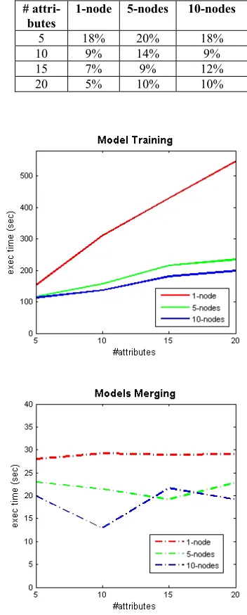
3092 Figure 9: Execution time of model training and merging

for 10 batches on 1, 5 and 10 nodes.

It can be observed on Figure 9 that:

(a) The execution times of model merging for 4 number of attributes are a lot smaller compared to the times of model training (see Table 5 for the percentages), and are relatively constant even though the size of batches varies. This is due to the fact the the models (being merged) are a lot smaller (10 to 15 Kb) than the batch size (0.5 to 2 Gb).

(b) Adding slave nodes to the Hadoop cluster improves the execution time. The larger the size of the batch (in the order of 550 Mb for 5 attributes, 1.1 Gb for 10 attributes, 1.6 Gb for 15 attributes and 2 Gb for 20 attributes), the wider the gap between time execution on a single node to on 5 and 10 nodes.

(c) The execution times of model training for processing batches are relatively constant. On the 5 and 10 slave nodes, by increasing the number of attribute and size of batch, the execution times are only slightly increased. But, there is fluctuation.

Table 5: Model merging/model training execution times.

# attri- butes

1-node 5-nodes 10-nodes

5 18% 20% 18%

10 9% 14% 9%

15 7% 9% 12%

20 5% 10% 10%

Figure 10: Average of execution times for batches with 5, 10, 15 and 20 attributes on 1, 5 and 10 nodes

On Figure 10, it is shown that:

3093 (b) The average of Job2 (models merging) execution time is relatively constant (with fluctuation) on the Hadoop cluster.

Thus, from these experiments, it can be concluded that:

(a) The MapReduce computation of Job1 for producing NBC models from batches is efficient and scalable. Adding nodes in the Hadoop cluster reduces the execution time. The fluctuation of the execution times are caused by the shuffling and sorting process over the network.

(b) The MapReduce computation of Job2 for merging the NBC models is also efficient and scalable. It runs a lot faster than Job1 as the model sizes being merged are a lot smaller than the batch size.

(c) The proposed parallel incremental NBC (consisting of Job1 and Job2) is efficient and scalable.

7. CONCLUSION AND FUTURE WORKS

The parallel classifiers for Hadoop and Spark that are grouped into eager learner can be further enhance to become incremental classifiers handling batches of preprocessed big data. All of the methods are potentially enhanced by adopting ensemble methods, which will be more efficient if implemented on Spark with its RDDs. Parallel Naïve Bayes classifier based on MapReduce that handles discrete attributes can be enhanced into an incremental classifier without implementing ensemble methods. Having the model be designed in the form of key-value pairs, it can be efficiently computed using MapReduce functions, by adopting MapReduce summarization and meta patterns, from batches of data. The old models can be merged with the newly created model (from the new batch) using MapReduce functions as well.

From the first experiment results, it is proven that the NBC single model can be computed incrementally based on the incoming batches of big data with accuracy that is approximately equal to the model built using the whole data at once. In testing the model, while the new case prediction can benefit from the mapper parallel efficient computation, the computation of measures are only handled by a single reducer. Computing confusion matrix, accuracy, precision, recall and f-measure needs to use the whole prediction results. In this research, all of these results are “collected” and processed by a single reducer only. Further research is needed to parallelize this computation.

From the second experiment results, it is shown that the proposed incremental NBC running on a Hadoop cluster is scalable and efficient. The time needed to merge the old model and the newly created model with a batch is a lot less then the model creation.

Further works: The incremental parallel classifier with ensemble methods need to be materialized such that preprocessed big data having continues as well as discrete attributes are handled efficiently. Big data may be in the format of texts, pictures, videos, graphs, encrypted, and so on. Developing parallel techniques to preprocess these kind of formats such that the results are ready to be classified is also required efficiently. Currently, we are researching methods for analyzing big graphs [20, 21, 22]. In the future we will develop the classifier for big graphs as well as encrypted big data.

ACKNOWLEDGMENT

This research is funded by Direktorat Riset dan Pengabdian Masyarakat, Direktorat Jenderal

Penguatan Riset dan Pengembangan (through

Penelitian Dasar Unggulan Pergurutan Tinggi scheme in 2019) and Parahyangan Catholic University (through Penelitian Dana Internal scheme in 2018). We would like to thank to them for their supports.

References

[1]. David Loshin, Big Data Analytics, Morgan Kaufmann Publ., USA, 2013.

[2]. A. Holmes, Hadoop in Practice, USA: Manning Publications Co., 2012.

[3]. C. Lam, Hadoop in Action, USA: Manning Publ., 2010

[4]. E. Sammer, Hadoop Operations, USA: O’Reilly Media, Inc., 2012.

[5]. D. Miner and A. Shook, MapReduce Design Patterns, O’Reilly Media, Inc., Sebastopol, CA, 2013.

[6]. J. A. Scott, Getting Started with Apache Spark: Inception to Production, MapR Technologies, Inc., USA, 2015.

[7]. H. Karau, A. Konwinski, P. Wendell & M. Zaharia, Learning Spark - Lightning-Fast Data Analysis, O’Reilly Media, Inc., Sebastopol, CA-USA, 2015.

3094 [9]. Y. Cui, Y. Yang and S. Liao, PDTSSE: A

Scalable Parallel Decision Tree Algorithm Based on MapReduce, School of Computer Science and Technology, Tianjin University, Tianjin, China, 2015.

[10]. P. Lucivnák, Parallel Implementation of

Dynamic Naive Bayesian Classifier,

Bachelor’s Thesis, Department of Theoretical Computer Science, CTU, Prague, May 9, 2018.

[11]. Q. He, F. Zhuang, J. Li, and Z. Shi, Parallel Implementation of Classification Algorithms Based on MapReduce, RSKT 2010, LNAI 6401, pp. 655–662, Springer-Verlag Berlin Heidelberg, 2010.

[12]. Y. Liu, W. Jing and L. Xu, Parallelizing Backpropagation Neural Network Using

MapReduce and Cascading Model,

Computational Intelligence and Neuroscience, Vol. 2016, Hindawi Publishing Corp., 2016. [13]. Z. Sun and G. Fox, Study on Parallel SVM

Based on MapReduce, Key Laboratory for

Computer Network of Shandong Province, Shandong Computer Science Center, Jinan, Shandong, China.

[14]. D. Xia, X. Lu, H. Li, W. Wang, Y. Li and Z. Zhang, A MapReduce-Based Parallel Frequent Pattern Growth Algorithm for Spatiotemporal Association Analysis of Mobile Trajectory Big Data, Complexity, Vol. 2018, Hindawi, 2018. [15]. B. Omar Alqarout, Parallel Text Classification

Applied to Large Scale Arabic Text, Faculty of Information Technology, The Islamic University of Gaza, State of Palestine, October 2017.

[16]. S. Lind, Distributed Ensemble Learning With

Apache Spark, Thesis, Molecular

Biotechnology Engineering, School of Engineering, Uppsala University, Sweden,2016.

[17]. A. A. Babu, J. Preethi, Incremental-Parallel Data Stream Classification in Apache Spark Environment, Proc. of 1st International Conference on Applied Soft Computing Techniques, April 2017.

[18]. V. S. Moertini, G. W. Suarjana, L. Venica and G. Karya, Big Data Reduction Technique using Parallel Hierarchical Agglomerative Clustering, IAENG International Journal of Computer Science, Vol. 45. No. 1, 2018. [19]. V. S. Moertini and L. Venica, Parallel k-Means

for Big Data: On Enhancing Its Cluster Metrics and Patterns, Journal of Theoretical and Applied Information Technology, Vol. 95, No. 8, 2017.

[20]. Atastina, I., Sitohang, B., Saptawati, G.A.P., Moertini, V.S., A Review of Big Graph Mining Research, Proc. of 2017 IOP Conference

Series: Materials Science and Engineering,

Bandung, Indonesia, 2017.

[21]. Atastina, I., Sitohang, B., Putri Saptawati, G.A., Moertini, V.S., An Implementation of Graph Mining to Find the Group Evolution in Communication Data Record, Proc. of 2018 ACM International Conference Proceeding Series, Singapore, 2018.

3095 APPENDIX A

Metrics for Evaluating Classification Model Performance

This appendix presents the definition and measure formulas for assessing the classifier model, which are implemented in ReduceTest function (Figure 8) excerpted from [8] (Han, Kamber & Pei, 2012).

When a classification model is used to test a set of labeled tuples, it is defined that P is the number of positive tuples (tuples of the main class of interest) and N is the number of negative tuples (all other tuples). Other definition:

a) True positives(TP): The positive tuples that were correctly labeled by the classifier. b) True negatives(TN): The negative tuples that

were correctly labeled by the classifier. c) False positives(FP): The negative tuples that

were incorrectly labeled as positive (e.g., tuples of class buys_computer_no for which the classifier predicted buys_computer_yes).

d) False negatives(FN): The positive tuples that were mislabeled as negative.

For a class having two values (yes and no), a confusion matrix is described as follows:.

Predicted class yes no Total Actual class yes TP FN P

no FP TN N Total P’ N’ P + N

For measuring the performance of classifier, four evaluation measures are defined as follows: a) accuracy (percentage of test set tuples that are

correctly classified) = (TP + TN) / (P + N) b) precision (what percentage of tuples labeled as

positive are actually such) = TP / (TP + FP) c) recall (what percentage of positive tuples are

labeled as such) = TP / P

d) F-measure (harmonic meanof precision and recall)= (2 x precision x recall) / (precision + recall)

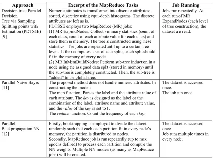
Table 1: MapReduce tasks and job on few parallel classification methods.

Approach Excerpt of the MapReduce Tasks Job Running

Decision tree: Parallel Decision

Tree via Sampling Splitting points with Estimation (PDTSSE) [9]

Numeric attributes is transformed into discrete attributes: sorted, discretize using equi-depth histograms. The discrete attributes are left as is.

PDTSSE employs two MapReduce (MR) jobs:

(1) MR ExpandNodes: Collect summary statistics (count of each class, count of each attribute value for each class) and store them in memory. The tree is constructed using these statistics. The jobs are repeated until up to a certain tree level. It then computes a set of data splits, each split should fit in the memory of every node.

(2) MR InMemBuildNodes: Perform sub-tree induction in a node using the assigned data split (stored in memory) until the sub-tree is completely constructed. Then, the sub-tree is “added” to the global-tree.

Jobs run repeatedly. At each run of MR

ExpandNodes (each level of tree construction), the dataset are read.

Parallel Naïve Bayes [11]

The proposed method does not handle numeric attributes. In constructing the model:

The map function: Parses the label and the attribute value of each attribute. The key is designed as the label or the combination of the label, attribute name and attribute value, and the value of the key is set to 1.

The reduce function: Count the frequency of each key.

The dataset is accessed once.

The job run once.

Parallel

Backpropagation NN [12]

Firstly, bootstrapping is employed to divide the dataset randomly such that each each partition fit in every node’s memory, the partition is distributed to nodes.

Secondly, MapReduce job is run repeatedly (up to max epochs defined) to process each partition and compute the NN weights. Multiple NN models (as many as MapReduce jobs) will be created.

The dataset is accessed once.