The London School of Economics and Political Science
Statistical Inference on Linear and Partly Linear Regression
with Spatial Dependence: Parametric and Nonparametric
Approaches
Supachoke Thawornkaiwong
Declaration
I certify that the thesis I have presented for examination for the Ph.D. degree of the London School of Economics and Political Science is solely my own work other than where I have clearly indicated that it is the work of others (in which case the extent of any work carried out jointly by me and any other person is clearly identi…ed in it).
The copyright of this thesis rests with the author. Quotation from it is permitted, provided that full acknowledgement is made. This thesis may not be reproduced without my prior written consent.
I warrant that this authorisation does not, to the best of my belief, infringe the rights of any third party.
I declare that my thesis consists of approximately 70000 words.
Statement of conjoint work
Abstract
The typical assumption made in regression analysis with cross-sectional data is that of independent observations. However, this assumption can be questionable in some economic applications where spatial dependence of observations may arise, for example, from local shocks in an economy, interaction among economic agents and spillovers.
The main focus of this thesis is on regression models under three di¤erent models of spatial dependence. First, a multivariate linear regression model with the disturbances following the Spatial Autoregressive process is considered. It is shown that the Gaussian pseudo-maximum likelihood estimate of the regression and the spatial autoregressive pa-rameters can be root-n-consistent under strong spatial dependence or explosive variances, given that they are not too strong, without making restrictive assumptions on the parameter space. To achieve e¢ ciency improvement, adaptive estimation, in the sense of Stein (1956), is also discussed where the unknown score function is nonparametrically estimated by power series estimation. A large section is devoted to an extension of power series estimation for random variables with unbounded supports.
Second, linear and semiparametric partly linear regression models with the disturbances following a generalized linear process for triangular arrays proposed by Robinson (2011) are considered. It is shown that instrumental variables estimates of the unknown slope parameters can be root-n-consistent even under some strong spatial dependence. A sim-ple nonparametric estimate of the asymptotic variance matrix of the slope parameters is proposed. An empirical illustration of the estimation technique is also conducted.
Acknowledgement
I would like to thank Professor Peter M. Robinson for his endless support, kindness and particularly his patience. I have learnt a great deal of econometrics and learnt to try to think more thoroughly from his detailed and substantive comments. He has been an immense source of good examples, inspiration, encouragement and support throughout my Ph.D. To him, I owe my deepest acknowledgements.
I would like to thank many individuals in the Econometrics group at the LSE during 2004 - 2008, in particular Professor Javier Hidalgo, Professor Oliver Linton, Dr. Marcia Schafgans and Dr. Myung Hwan Seo for lively discussions and support.
I also would like to thank many individuals who previously taught me mathematics, statistics, econometrics and economics, particularly Dr. Javier Hualde who gave an excellent introductory course in econometrics. His impressive teaching has played an important role in shaping my academic path towards research in econometrics.
An endless support form Mark Wilbor, the MRes-PhD in Economics Programme Man-ager, is appreciated.
I would like to thank the Bank of Thailand for the scholarship during the …rst year of my doctoral study and the LSE for the scholarship during the 2nd, 3rd, and 4th years of my study.
Chapter 2 of the thesis was written from May through early August 2012. The author will not be able to complete this chapter without the kind permission from many executives at the Bank of Thailand to take a leave from mid June to mid August.
Contents
Title page 1
Declaration 2
Abstract 3
Acknowledgements 4
Contents 5
List of Tables and Figures 7
Chapter 1: Introduction 8
Chapter 2: Likelihood Based Inference on Multivariate Regression with 11 Spatial Autoregressive Disturbances
2.1Introduction 11
2.2Spatial autoregressive model 13
2.2.1 Univariate spatial autoregressive model 13
2.2.2 Multivariate spatial autoregressive model 16
2.3Multivariate linear regression 18
2.3.1 Consistency 20
2.3.2 Asymptotic normality 22
2.4Nonparametric Series Estimation 28
2.5E¢ ciency Improvement 37
2.6Final Comments 44
Appendix 2.1: Proofs of Theorems 45
Appendix 2.2: Propositions for Proof of Theorem E 56 Appendix 2.3: Technical Lemmas for proofs of Theorems 61
Chapter 3: Statistical Inference on Regression with Spatial Dependence 98
3.1Introduction 98
3.2Linear Regression 99
3.3Partly Linear Regression 102
3.5Monte carlo study of …nite-sample performance 112
3.6Empirical Illustration 114
3.7Final comments 118
Appendix 3.1: Proofs of Theorems A and B 119
Appendix 3.2: Propositions for proofs of Theorems A and B 120 Appendix 3.3: Technical Lemmas for proofs of Theorem A and B 124
Appendix 3.4: Proof of Theorem C 137
Chapter 4: Linear Analysis with Irregularly Spaced Data 147
4.1Introduction 147
4.2Models 149
4.2.1 Background on point processes 150
4.2.2 Second-order stationary point processes 151
4.2.3 Wide-sense second-order stationary random signed measure 152 4.3Asymptotic properties of random signed measures 155
4.3.1 Weak law of large numbers 155
4.3.2 Central limit theorem 156
4.3.3 van Hove convergence 156
4.4Least squares estimation 158
4.5Spectral density estimation 160
4.5.1 Bias 162
4.5.2 Variance 163
4.6Positive de…nite estimate 165
4.7Final comments 168
Appendix 4.1: Proofs of Theorems 169
Appendix 4.2: Technical Lemmas for proofs of Theorems 179
List of Tables and Figures
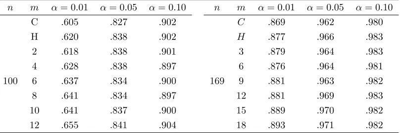
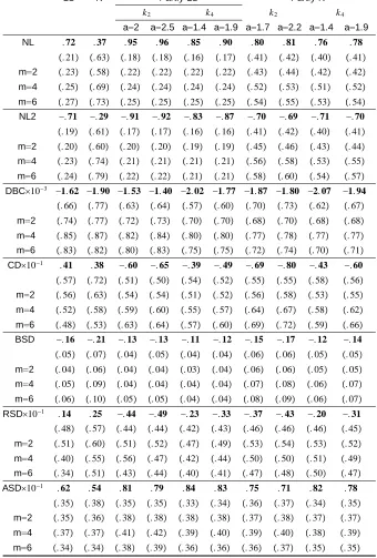
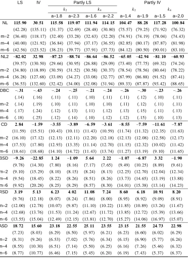
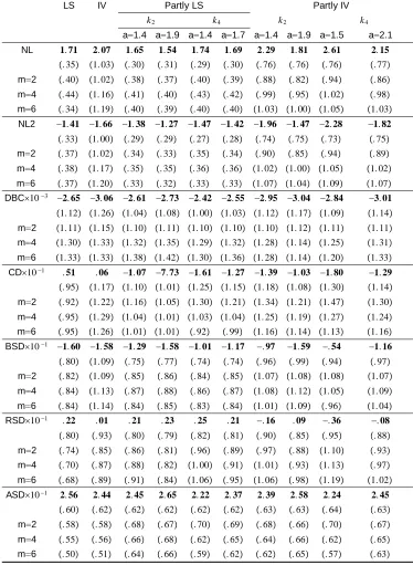
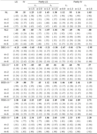
Table 1: Linear regression (3.1): Empirical sizes of tests with size 138 Table 2: Linear regression (3.1): Empirical powers of tests with 138
= 0:8 and size
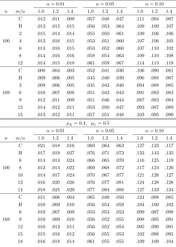
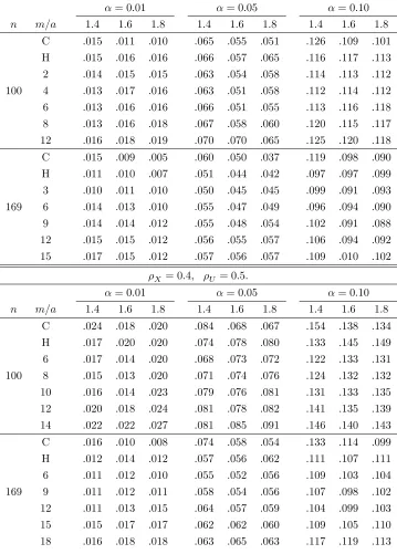
Table 3: Partly linear regression (3.5): Empirical sizes of tests 139 with size usingk2
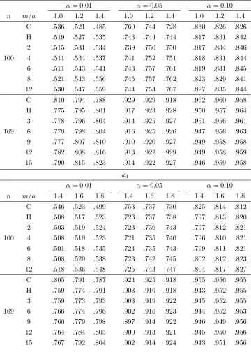
Table 4: Partly linear regression (3.5): Empirical sizes of tests 140 with size usingk4
Table 5: Partly linear regression (3.5): Empirical powers of tests 141 with = 0:7 usingk2; k4at level
Table 6: Y =Proportion of irrigated land (IR) 142
Table 7: Y =Fertilizer use (FU) 143
Table 8: Y =Log(yield 15 major crops) (L15) 144
Table 9: Y =Log(rice yield) (LR) 145
Figure 1: Nonparametric regression 1 146
Figure 2: Nonparametric regression 2 146
Figure 3: Nonparametric regression 3 146
1
Introduction
Modern econometrics can, to some extent, be regarded as a branch of mathematical statis-tics aimed at providing statistical tools for economic analysis. Traditionally, cross-sectional data were analysed in microeconomic studies whereas time series data were employed in the macroeconomic counterpart. However, this distinction is no longer prevailing. There has been a rather signi…cant movement among macroeconomists to collect and analyse cross-sectional data in order to understand macroeconomic behaviours. Household expenditure surveys have played a crucial role in helping macroeconomists understand consumption and saving behaviours. Surveys of consumer …nances have also become popular for empirical analysis of asset pricing. Investment and R&D data at …rm levels have improved macro-economists’understanding of investment and R&D decisions, which play a role in short-term economic ‡uctuations and are widely accepted as being vital for economic growth. Cross-sectional data are currently playing key roles in other areas of studies such as unemployment and credit markets too.
There are many reasons explaining the popularity of cross-sectional data in macroeco-nomic analysis. Given that most macroecomacroeco-nomic theories are currently based on microeco-nomic foundations, which focus on decisions of ecomicroeco-nomic agents in an economy, it is vital to check at the right level, e.g. households or …rms, whether such theories are valid. Moreover, cross-sectional data are particularly useful for policy evaluation such as e¤ects of minimum wages and monetary policy. If one were to rely on aggregate data, one would have to analyse only a few data points whereas the micro-level data can give a great deal of information.
The reader may be thinking of panel data and consider them as being di¤erent from the cross-secional one. However, given that most panel data used in economic analysis have much shorter time span compared with the number of cross-sectional observations, this type of panel data can be regarded, from the theoretical point of view, as cross-sectional data with higher dimensions. Hence the theories developed for cross-sectional data will be applicable to panel data (over a short time span) too. A serious discussion of panel data with large cross-sectional observations over a long period of time requires a proper theoretical foundation for spatio-temporal dependence, which is beyond the scope of this thesis.
the physical one.
There are two main strategies in econometric literature aimed at modelling spatial de-pendence. The …rst line of research is based on the idea that a family of random variables exhibiting spatial dependence can be represented as a linear process with independent inno-vations. The most popular parametric model on this line of research is the Spatial Autore-gressive (SAR) model. Recently Robinson (2011) proposed a generalized linear process for a triangular array of random variables and showed that a broad class of spatial processes can be represented by such a generalized linear process. It should be stressed that the generalized linear process of Robinson (2011) is a nonparametric model. The advantage of this modelling strategy is that many well-established results from linear time series can be extended.
The other line of research is to assume that the data is, to some degree, second-order stationary. Conley (1999) considered irregularly spaced data inR2. He assumed that the data is a marked point process where the marks and the ground process are independent. Moreover, he assumed that the marks are stationary random …elds and the ground process is a hard-core process. The assumption that the ground process is a hard-core process allows researchers to regard irregularly spaced spatial data onR2 as a random …eld on the lattice Zd, where Zd is the Cartesian d-product of the space of integers Z. Even though Conley (1999) was able to show analytical tractability of his model, his assumptions on the hard-core process is restrictive and result in computationally intensive calculation.
In this thesis, we investigate both lines of researches. In Chapter 2, we investigate a mul-tivariate linear regression model with the disturbances following a mulmul-tivariate SAR model. The parametric set-up of the SAR model allows us to employ likelihood based inference. We …rst consider the Gaussian pseudo-maximum likelihood estimate of the unknowns. We show that under mild regularity conditions, such estimate can be root-n-consistent. Our regularity conditions are quite di¤erent from the ones in the existing literature. First, we do not impose excessive restriction on the parameter space. Second, we show and stress analytical tractability and ‡exibility of the spectral norm compared with thek k1 andk k1 norms commonly employed in the literature. Employing a di¤erent technique for proof of consistency of the estimate, we can avoid row or column normalization. We also allow the SAR process to exhibit long-range dependence or explosive variances while the existing literature focuses on short-range dependence and bounded variances. The Gaussian pseudo-maximum likelihood estimate will lose its e¢ ciency if the innovations of the SAR process are not normally distributed. This leads us to consider e¢ ciency improvement of the Gaussian pseudo-maximum likelihood estimate by nonparametrically estimating the unknown score function of the distribution of the innovations. This "adaptive" estimate of the slope para-meters of the regression is asymptotically as e¢ cient as the one obtained from the maximum likelihood estimation when the density function is known. Our nonparametric estimate of the unknown score functions is a power series nonparametric estimate. In order to allow the number of approximating functions to increase faster than the ones in the literature, we employ properties of orthonormal polynomials in our proof. We also extend some results in power series literature to allow for random variables with unbounded support.
distur-bances follow a generalized linear process in Robinson (2011). Central limit theorems are developed for instrumental variables estimates of linear and semiparametric partly linear regression models. We also show that the estimate of the slope parameters in the linear part of the partly linear model can be root-n-consistent similar to the case for independent data. We discuss estimation of the variance matrix, including estimates that are robust to disturbance heteroscedasticity and/or dependence. A Monte Carlo study of …nite-sample performance is included. In an empirical example, the estimates and robust and non-robust standard errors are computed from Indian regional data, following tests for spatial corre-lation in disturbances, and nonparametric regression …tting. Some …nal comments discuss modi…cations and extensions.
2
Likelihood Based Inference on Multivariate
Regres-sion with Spatial Autoregressive Disturbances
2.1
Introduction
In this chapter, we consider a parametric model employed to capture spatial dependence. The most popular parametric model in econometric literature is the Spatial Autoregressive (SAR) model introduced by Cli¤ and Ord (1973) and popularised by Anselin (1988). The simplest SAR model for a triangular array of random variablesfui;n; 1 i n; n 1g is of the form
ui;n= 0 n X
j=1
wij;nuj;n+"i; (2.1)
where 0 is the spatial autoregressive parameter, wij;n are nonstochastic weights andf"ig is a sequence of uncorrelated random variables with zero mean and constant variance 20. For simplicity, the subscript n will be omitted from the presentation. The model in (2.1) can be re-written in a matrix form as
u= 0W u+"; (2.2)
where u = (u1; :::; un)0; W is the n n matrix whose (i; j)-th element is wij; " =
("1; :::; "n)0 and the prime0 denotes transposition. The model in (2.2) can be re-written as
Su= (In 0W)u=";
where S=In 0W. If 0 takes a value such thatS is invertible, then the model implies that
u=S 1" and V ar(u) = 20(S0S) 1:
Unlike in time series analysis, it may not be obvious for practitioners how the weights
wij should be chosen. One natural choice of the weights is to rely on "economic" distances of each pair of observations. In this case, the weights should have inverse relationships with distances to re‡ect falling-o¤ dependence as distances increase. However, the row-normalisation restriction, i.e.
wij=
f(dij) Pn
j=1f(dij)
;
Practitioners may …nd restrictions on both the parameter space of 0 and on W too restrictive. In many applications, practitioners may prefer a symmetric matrix re‡ecting distances between economic agents or observations, i.e. wij =f(dij), wheredij is the dis-tance between thei-th andj-th obsevations, as a natural choice of the weighting matrix. In this case, row or column normalisation will be restrictive. Moreover, when a chosen func-tionf is known up to an unknown scale, the unknown scale can be absorbed by the spatial autoregressive parameter 0. This implies that a further restriction commonly imposed on the parameter space of 0 will become restrictive.
In this paper, we also show that the assumptions imposed in the existing literature do not cover two important scenarios, namely explosive variances of some observations and long range dependence.
In this paper, we show that these restrictions are unnecessary to obtain a root-n-consistent estimate of the unknown autoregressive parameter. Instead of considering a simple univariate SAR model, we consider a multivariate linear regression model with SAR disturbances. We show that with Gaussian pseudo-maximum likelihood estimation, we can obtain a root-n-consistent estimate of the unknown parameters under long-range spatial dependence or explosive variances.
When the innovations "i are i.i.d., we also show how to obtain e¢ ciency improvement over the Gaussian pseudo-maximum likelihood estimate by nonparametrically approximate the unknown score function of the distribution of the innovations. Our e¢ cient estimate is based on series approximation of the unknown score function suggested by Beran (1976) for …nite dimensional cases. This estimate is computationally simple and the issue of se-lecting the trimming parameter can be avoided. In order to nonparametrically estimate the unknown score function in a general in…nite-dimensional space, one has to allow the number of approximating functions to increase to in…nity at an appropriate rate. Newey (1988) extended Beran’s technique to obtain an adaptive estimate of the slope parameters of a linear regression model with i.i.d. data but the number of approximating functions has to go to in…nity at a rate that is slower than logarithm of the sample size. Robinson (2005), considering e¢ cient estimation of time series regression with fractional disturbances, showed that the condition in Newey (1988) can be relaxed and allow the number of approximating functions to increase at the rates slightly faster than that in Newey (1988).
In this paper, we show that in order to obtain an e¢ ciency improvement of an estimate of the slope parameter in a multivariate linear regression with SAR disturbances, the number of approximating functions can indeed increase with the sample size at a polynomial rate. The proof relies on results from power series approximation literature. Unlike other papers in the literature, we show that in order to allow the number of approximating power functions to grow at the rate that is proportional to a fractional power of the sample size, we do not need to make a restrictive assumption that the density function of the disturbances must have bounded support. The result in this chapter should be applicable to other semiparametric models in econometrics, where the power series approximation is employed to estimate the nonparametric part of a model.
maximum column sum and maximum row sum norms commonly employed in the literature. We also discuss how to relax the condition on uniform boundedness of row and column sums to possibly allow for long-range dependence or explosive variances. Some further analytically tractable results can be obtained when W is symmetric. In section 3, we discuss consistency and asymptotic normality of the Gaussian pseudo-maximum likelihood estimate of a multivariate linear regression model with multivariate SAR disturbances. In section 4, we extend some results in nonparametric series approximation to allow for random variables with unbounded support. Finally, e¢ ciency improvement of the slope parameter in the multivariate linear regression model is discussed. Proofs and technical lemmas are left in the Appendices.
2.2
Spatial Autoregressive Model
In this section, we discuss a spectral norm and show its analytical tractability for the SAR model. First, we introduce some notations. Let A be an n n matrix and aij de-note its (i; j)-th element. De…ne (A) and (A)as the largest and smallest eigenvalues of
A; respectively. De…ne kAk1 = max1 j nPni=1jaijj; kAk1 = max1 i nPnj=1jaijj; and
kAk= (A0A) 1=2:Let (A) = maxfj j: is an eigenvalue ofAg and jAjbe the deter-minant ofA:In this chapter, a square matrix Aof ordernis positive de…nite (p.d.) ifAis symmetric and for anyx2Rn such thatx6= 0; x0Ax >0. Similarly, a square matrix Aof ordernis positive semide…nite (p.s.d.) if Ais symmetric andx0Ax 0for anyx2Rn:
2.2.1 Univariate Spatial Autoregressive Model
Consider a univariate SAR model in (2.2). As mentioned in the previous section,V ar(u) = 2
0(S0S) 1
: The most common assumption in the literature, as in Kelejian and Prucha (1998) and Lee (2004), is
Assumption A1 S 1
1+ S
1
1 is bounded uniformly inn.
Since it can be shown that both k k1 and k k1 are matrix norms as de…ned in Horn (1985), one implication of this condition is thatkV ar(u)k1+kV ar(u)k1 is bounded uni-formly in n: Now consider the spectral norm. One advantage of the spectral norm can be seen directly from Lemma A1 that for any square matrixA; kAk =kA0k: In order to get an analogous result on a bound for V ar(u), by employing the spectral norm, we need to make the following condition.
Under Assumption A2, S0S is p.d. and hence (S0S) 1 = f (S0S)g 1: Because
kAk=kA0k;Assumption A2 is equivalent to the condition that S 1 is bounded uniformly inn:As(S0S) 1
is p.d., by Lemma A3, (S0S) 1
= (S0S) 1
. Therefore, Assumption A2 is also equivalent to the condition that (S0S) 1 andkV ar(u)kare bounded uniformly inn: AsV ar(u)is symmetric, by Lemma A3,
kV ar(u)k kV ar(u)k1 and kV ar(u)k kV ar(u)k1:
Therefore Assumption A1 implies Assumption A2. If variance matrices are of primary concern, the following theorem shows that the spectral norm is strictly weaker than k k1 andk k1 norms.
Theorem A Consider any familyfAngof positive de…nite matrices of ordern:(i)kAnk
kAnk1 andkAnk kAnk1:(ii) There exists a family fAng such that kAnk are uniformly bounded inn butkAnk1 andkAnk1 are not.
Even though Assumption A2 is weaker than Assumption A1 that is commonly employed in the literature, it may be too strong. With reference to time series literature, consider a covariance stationary processfvtg:One possible nonparametric de…nition for long-range dependece offvtgis that
V ar n 1=2
n X
t=1 vt
!
! 1; as n! 1: (2.3)
Letz=n 1=2(1; :::; 1)0be a vector inRn:Sincen 1=2Pn
t=1vt=z0vwherev= (v1; :::; vn)0; it follows that V ar n 1=2Pnt=1vt = z0V ar(v)z; where kzk = 1: Since z0V ar(v)z
kV ar(v)k, then kV ar(v)k ! 1; as n ! 1 given that fvtg has long-range dependence. Alternatively, supposefvtghas absolutely continuous spectral distribution and letf be the density function. It is common to say thatfvtg has short memory if
0< f( )<1; for all 2[ ; ): (2.4)
Note that this de…nition excludes seasonal long memory. If fvtg has short memory as de…ned in (2.4), then one observation in section 5.2 (b) in Grenander and Szego (1984) implies thatkV ar(v)k is bounded uniformly in n:These two results suggest that uniform boundedness of kV ar(v)k can be a rather sensible description of time series exhibiting short-range dependence.
Given these results one may be tempted to say that a SAR process u has long range dependece if
It is clear that Assumption A2 does not allow for this possibility. This may be a serious drawback of Assumption A2 since some spatial data may be subject to long-range depen-dence. Fari…eld Smith (1938) mentioned the problem of (2.3) when analysing agricultural spatial data. However, this de…nition may be misleading since it is possible that (2.5) holds whenV ar(ui)! 1as n! 1for someibut Cov(ui; uj)becomes arbitrarily small su¢ -ciently fast as the distance between thei-th andj-th observations increases. In other words, condition (2.5) may arise not from long-range dependence but from explosive variances of some observations. Neverthess, this explosive behaviour of the variances may arise naturally in some economic applications. With reference to economic geography literature, agglomer-ation of economic activities in a certain locagglomer-ation may be a norm rather than an exception to bene…t from economies of scales. See Fujita, Krugman and Venables (2001) for a reference. Hence concentration of economic activities may be sources of explosive variances.
AsS=In 0W, Lemma A4 implies that is an eigenvalue ofSif and only if = 1 0! where! is an eigenvalue of W:If 0= 0, then S =In and we have a trivial case. Suppose 0 6= 0, then S is invertible, i.e. 6= 0; as long as none of the eigenvalues ofW is equal to 1= 0: Non-singularity of S can be regarded as an identi…cation restriction so that each ui can be written uniquely as a linear combination of "j: It is generally di¢ cult to have much information aboutkV ar(u)ksince it depends on the unknown 0and the relationship betweenV ar(u)and 0 may be highly nonlinear. However, ifW is symmetric, for example when economic distances are employed to constructWwithout row or column normalization, many analytically tractable results can be obtained.
If W is symmetric, then S and S 1 are symmetric. Lemma A5 also implies that kV ar(u)k = 20max
n
(1 0!) 2
:!is an eigenvalue of Wo: Even though S is assumed to be non-singular, kV ar(u)k can becomes arbitrarily large if at least one of the eigenval-ues of W gets arbitrarily close to1= 0 as n ! 1: The rate at which kV ar(u)k becomes explosive depends on the rate at which one of the eigenvalues ofW gets arbitrarily close to
1= 0: In other words, for a given 0; the explosive behaviour ofkV ar(u)k depends on the characteristic values of the weight matrixW:
Compared with the symmetric case, kV ar(u)k loses its analytical tractability whenW
is not symmetric. The complexity ofkV ar(u)kwhenW is not symmetric can be illustrated from the truncated …rst-order autoregressive model. Letx1="1andxt= xt 1+"t; t 2; where f"tg is a white noise process. Then it can be shown that x= (x1; :::; xn)0 can be represented as in (2.2) withwij = i;j+1, where ij is the Kronecker’s delta. It follows that the resulting weight matrixW is a lower shift matrix and is also nilpotent. Hence, every eigenvalue ofW is equal to zero and, by Lemma A4, every eigenvalue ofS is equal to unity regardless of the value of 0: This implies thatS is always invertible and every eigenvalue of S 1 is equal to unity regardless of the value of
0: However, when 0 = 1; i.e. fxtg is a truncated random walk process, kV ar(x)k becomes explosive at a fairly fast rate. This example illustrates the di¢ culty in determining the behaviour of kV ar(u)k particularly whenW is not symmetric.
Lemmas A1 and A10 in the Appendix thatkV ar(u)k is proportional to
(S0S) 1 = S 1 S 1 0 S 1 2:
Lemma A2 shows that this inequality becomes an equality when W is symmetric. When
W is not symmetric, one can at least conclude that if S 1 is explosive, then (S0S) 1 is also explosive. One can only infer that the rate at which (S0S) 1
becomes explosive is at least as fast as the rate of S 1 2. However, a sharper rate at which (S0S) 1 becomes explosive may not be easy to conclude. The truncated random walk process is a good example showing this complexity.
De…ne G = W S 1. It will be clear later that G arises naturally from the Gaussian psuedo-maximum likelihood estimation of the unknown 0: If 0 = 0, then G = W. It follows form the proof of Lemma A6 that if 06= 0;
G= 01 S 1 In : (2.6)
This equality shows that when there is spatial dependence, i.e. 0 6= 0; the matrix 0Gis essentially the matrixS 1:Recall thatu=S 1". It follows thatu
i=Pnj=1bij"j wherebij is the(i; j)-th element ofS 1:Following (2.6), thei-th element of
0G"is Pn
j=1bij"j "i: That is 0G"is essentially the same asu. Moreover, Lemma A6 indicates that
S 1 1 k 0Gk= S 1 + 1:
Hence kGk j 0j 1 S 1 as S 1 ! 1, where ‘ ’ indicates that the ratio of left and right sides tends to1:Note that S 1 can get arbitrarily large only if
06= 0:
2.2.2 Multivariate Spatial Autoregressive Model
In a multivariate case, we havenobservations andgequations. The univariate SAR model in (2.1) can be generalized to
uit= 0t n X
j=1
wijtujt+"it; i= 1; :::; n; t= 1; :::; g; (2.7)
where the indexiis associated with thei-th observation and the index tis associated with thet-th equation. In a matrix form, this can be written as
ut= 0tWtut+"t; t= 1; :::; g; (2.8) where ut = (u1t; :::; unt)0, "t = ("1t; :::; "nt)0 and Wt is the matrix whose (i; j)-th ele-ment iswijt: This speci…cation assumes no direct cross-equation e¤ects but cross-equation dependence arises from dependence structure of ("i1; "i2; :::; "ig)0: For square matrices
can be re-written as
u=diag 01W1; :::; 0gWg u+";
whereu= u0
1; :::; u0g 0 and"= "01; :::; "0g 0:De…neSt=In 0tWt, then
Su=";
whereS=diag(S1; :::; Sg):
Assumption B1 Fort= 1; :::; g; Wtaren nmatrices of nonstochastic weightswijtand
St are non-singular for alln 1:
Let1be the indicator function.
Assumption B2 Let"i = ("i1; :::; "ig)0:(i)E("i) = 0for alli:(ii)E "i"0j = 01(i=j) for alli; j; where 0 is p.d..
Under Assumptions B1 and B2,
u=S 1";
whereS 1=diag S11; :::; Sg1 ;
V ar(") = 0 In;
where is the Kronecker product, and
V ar(u) =S 1( 0 In) S 1 0= S0 01 In S 1
:
It follows from Lemmas A1 and A7 that
kV ar(u)k k( 0 In)k S 1 2=k 0k S 1 2:
If (2.5) holds, then it must be the case that
S 1 ! 1asn! 1:
Hence S 1 is the source of an explosive behaviour ofkV ar(u)k. Lemma A8 implies that S 1 = max
1 t g St1 . This simple relationship suggests that the results previously established for a univariate process can be applicable to a multivariate process. Similarly, we can de…neG=diagfG1; :::; Gggwhere Gt=WtSt1: Lemma A8 implies thatkGk=
2.3
Multivariate Linear Regression
In this paper we consider a multivariate linear regression model
yit=x0it 0+uit; i= 1; :::; n; t= 1; :::; g;
whereyitare scalar random variables,xitareRK-valued random variables, 0are unknown vectors inRKand the disturbancesu
itfollow a multivariate SAR process as de…ned in (2.7). Then, for eacht= 1; :::; g;we have
yt=Xt 0+ut;
where yt = (y1t; :::; ynt)0, Xt = (x1t; :::; xnt)0 and ut = (u1t; :::; unt)0: This can be written as
y=X 0+u;
wherey= y0
1; :::; y0g 0
; X = X0
1; :::; Xg0 0
andu= u0
1; :::; u0g 0
:
Under the assumption that f"ig; as de…ned in the previous section, is a sequence of independent vectors of jointly normally distributed random variables with zero mean and
V ar("i) = 0, and the assumption that the regressors xit and"js are independent for all
i; j; tand s;and that the distributions of xit do not depend on 0; 0 and 01; :::; 0g; the log-likelihood function of y for the maximum likelihood estimation of the unknown parameters is
ln( ; ; ) =
ng
2 log 2 + 1
2log S( )
0S( ) 1
2logj Inj 1
2u
0( )S0( ) 1 I
n S( )u( );
where = 1; :::; g 0; St( ) =In tWt; S( ) =diag(S1( ); :::; Sg( ));andu( ) =
y X :
If the normality assumption does not hold, we can employ this log-likelihood function to construct a loss function
Qn( ; ; ) =
1 2glog
1 1
2ng
g X
t=1
log St( )0St( ) (2.9)
+ 1 2ngu( )
0S( )0 1 I
n S( )u( ):
Letb; b andbbe the minimizer of this loss function. Given and , the minimizer b( ; ) = X0S( )0 1 In S( )X
1
X0S( )0 1 In S( )y:
If we ignore symmetry of , then, applying the relationship that
it follows that
b( ) = arg min 2Rg g
1
2glogj j+ 1 2ngtr
( 1
n X
i=1
"i b; "i b;
0!)
; (2.10)
where
("1t( ; ); :::; "nt( ; ))0 ="t( ; ) =St( )ut( )
and "i ( ; ) = ("i1( ; ); :::; "ig( ; ))0:For each i; "i b; "i b; 0
is p.s.d. re-gardless of the values of . Asnincreases it is more likely thatPni=1"i b; "i b;
0
is p.d. and hence singular. Then we can apply Lemma 3.2.2 in Anderson (2003) to show that
b( ) = 1 n
n X
i=1
"i b; "i b; 0
: (2.11)
Note that there is a typographical error in the statement of Lemma 3.2.2. There should be " " in front of NlogjGj. Moreover, the same Lemma implies that the minimum value of the objective function in (2.10) is
C 1
2glog b( ) ;
whereC is a constant. Hence
b= arg min 2Rg
1
2glog b( ) 1 2ng
g X
t=1
log St( )0St( ) :
Now we give a formal statement for the minimisation problem. Following Abadir and Magnus (2005), for any symmetric matrixAof orderg, de…ne the half-vec ofA,vech(A);as the g(g+ 1)=2 1 vector that is obtained from vec(A) by eliminating all supradiagonal elements of A: Let = 01; 02; 03 0 where 1 = ; 2 = vech 1 and 3 = =
1; :::; g 0
:
Let
b= arg min 2
Qn( );
data model that is essentially a multivariate model. However, Lee and Yu (2010) assumed that =Ig; Wt=W and t= for allt= 1; :::; g:This assumption essentially simpli…es a multivariate SAR model to a univariate one.
2.3.1 Consistency
To show consistency ofb; we make the following assumptions. LetNbe the set of natural numbers.
Assumption B3 f"igis a sequence of independent Rg-valued random variables such that (i)E("i) = 0for all iinN:(ii) E("i"0i) = 0 for alliinN;where 0 is a positive de…nite matrix. (iii) There is a …nite constantC such that
max
1 t gmaxi 1 E" 4 it C:
Assumption B4 is a compact set. In addition, 2 is a subspace ofRg(g+1)=2 such that is positive de…nite for allvech( )2 2:
For any positive de…nite matrixA, letA1=2be the square root matrix ofA:De…ne H( 2; 3) = 10=2 In S 1 0S( )0 1 In S( )S 1 10=2 In :
By de…nition, H( 2; 3) is positive semide…nite for all 2 2 2 and all 3 2 3: The matrix Gt de…ned in the previous section can be written as G = W S 1; where W =
diagfW1; :::; Wgg.
Assumption B5 Let 1; :::; ng be eigenvalues of H( 2; 3):For any >0, there exists >0 such that for someN;
inf k 0k
( 1 ng
ng X
i=1
( i log i 1) )
;
for alln N;where = 02; 03 02 2 3:
Assumption B6 (i)fxitg andf"itg are independent. (ii) Let X =SX and hence Xt =
StXt: Asn! 1;
1 ng
X 0 s
Xs0G0s !
Xt GtXt !p
Qst 11 Qst12 Qst21 Qst22 !
and
1 ng
(X )0 01 In X (X )0 01 In GX
(X )0G0 01 In X (X )0G0 01 In GX !
!p
O11 O12 O21 O22 !
;
whereO11 is p.d..
Let vij be the (i; j)-th element of the G0G, (xit)0 be thei-th row of Xt, (xit)0 be the
i-th row ofXt =GtXt anduit be thet-th element of ut=Gtut:
Assumption B7 Asn! 1;
ng X
i=1 ng X
j=1
v2ij =o n2
and for any s; t= 1; :::; g;
n X
i=1 n X
j=1
E xis xjt 0 Cov uis; ujt = o n2 ;
n X
i=1 n X
j=1
E xis xjt 0 Cov uis; ujt = o n2 :
Theorem B Under Assumptions B1 and B3-B7,b!p 0:
Assumption B4 on 2 may appear to be quite restrictive. However, (2.11) shows that without the assumption on positive de…niteness of , an unconstrained optimizer for 2 gives b that is always positive semide…nite and usually positive de…nite in …nite samples. Hence Assumption B4 is not really a practical issue.
Assumption B5 is quite common in multivariate analysis. Consider a functionf :R+! Rwheref(x) =x logx 1:We have thatf(x)>0for allx >0exceptx= 1andf(1) = 0:
Hence 1 ng
Png
i=1( i log i 1) = 0if and only if i= 1fori= 1; :::; n. This is equivalent to H( 2; 3) = In. Note that H( 02; 03) = In: Assumption B5 essentially states that when is su¢ ciently di¤erent from 0,H( 2; 3)is su¢ ciently di¤erent fromH( 02; 03): There is one technical issue with Assumption B5. There may be some = 3 2 3 such thatS( )is singular. In this case, there is i = 0;where i is an eigenvalue ofH( 2; 3), and hence log i is not generally well de…ned. However, we employ the rule stated earlier that we de…nelogx= 1ifx= 0:It is worth noting that Assumption B5 is for asymptotic identi…cation of 2and 3:
As can be seen in the proof of Theorem B, we can easily avoid considering the term
S( ) 1. Therefore we do not need to impose any assumption on 3so thatS( )is invertible for any 2 3 as in the literature. With reference to (2.9) any value of making S( ) singular cannot be a minimizer of Qn( ) since we set logx= 1for x= 0: Hence these values of will be automatically removed from the "e¤ective" parameter space when doing an optimization problem.
The most important point to be noted here is that we do not assume any bound on
S( ) 1 uniformly in 3 as in the literature. The discussion at the end of Section 2 implies that Assumption B7 allows S 1 and hencekV ar(u)k to be explosive but at an appropriate rate. Since S 1 and G depends only on 0, our assumptions are imposed on the true value 0 but not the whole parameter space of 0: As discussed at the end of Section 2,Gis essentiallyS 1. In a univariate case, sinceV ar(u) = 2
0 S 1 0S 1 , in the presence of spatial dependence,G0Gis essentiallyV ar(u):Hence Assumption B7 allows the variance matrix ofuto be explosive but the rate at which it becomes explosive cannot be too fast. Moreover, in the presence of spatial dependence, i.e. 0t6= 0, Gt = 0t1 St1 In : Then
Xt =GtXt = 0t1Xt 0t1Xt andut=Gt"t= 0t1ut 0t1"t: Hence the latter part of Assumption B7 is equivalent to
n X
i=1 n X
j=1
E xis(xjt)0 Cov(uis; ujt) = o n2 ;
n X
i=1 n X
j=1
E xis xjt 0 Cov(uis; ujt) = o n2 :
This is the limit on the joint explosive behaviour of the regressors and disturbances.
2.3.2 Asymptotic Normality
First we introduce notations employed in this part. Fort= 1; :::; g;recall thatXt is de…ned asStXt. Let(xit)0 be thei-th row ofXt:Fors; t= 1; :::; g;let st0 and stbe the(s; t)-th element of 01 and 1, respectively. Similarly, let 0st and st be the(s; t)-th element of 0and , respectively. De…neut( ) =yt Xt and st( ) =us( )0Ss( )0St( )ut( ): Let ( )be the square matrix whose (s; t)-th element is st( ): Fort = 1; :::; g;letgijt be the (i; j)-th element of Gt: For any value of such that St( ) is non-singular, de…ne
Gt( ) =WtSt1( ) and G( ) = diag(G1( ); :::; Gg( )): Following Abadir and Magnus (2005), for any symmetric matrix A of order n; de…ne the duplication matrix Dn as the
n2 n(n+ 1)=2 matrix such that D
nvech(A) = vec(A): De…ne st as the Kronecker’s delta.
sym-metric. With reference to Lemmas C1 and C2, the …rst derivatives are
@Qn( )
@ 1
= 1
ngX
0S( )0 1 I
n S( )u( ); (2.12)
fors t;
@Qn( )
@ st =
2 st
2g st+ 2 st
2ng st( ); (2.13)
and fort= 1; :::; g; @Qn( )
@ 3t
= 1
ngtrfGt( )g 1 ng g X s=1 stu
s( )0Ss( )0Wtut( ); (2.14) where 3tis thet-th element of 3: Note that (2.13) can be written in a matrix form as
@Qn( )
@ 2
= 1
2gD 0
gvec( ) +
1 2ngD
0
gvec( ( )); (2.15)
whereDg is the duplication matrix.
It follows from (2.12), (2.15) and (2.14) that
@Qn( 0) @ 1
= 1
ng(X )
0 1
0 In ";
@Qn( 0) @ 2
= 1
2gD 0
gvec( 0) + 1 2ngD 0 gvec 0 B B @ "0
1"1 "01"g ..
. . .. ...
"0
g"1 "0g"g 1 C C A;
and fort= 1; :::; g;
@Qn( 0) @ 3t
= 1
ngtr(Gt) 1 ng g X s=1 st
0"0sGt"t:
Let
n = ngE
@Qn( 0) @
@Qn( 0)
@ 0 X
= 0 B @
11;n 12;n 13;n 21;n 22;n 23;n 31;n 32;n 33;n
1 C A;
where ij;n=E @Q@n(i0)@Q@n(0 0)
j X :
By Assumption B6,
11;n=
1 ng(X )
0 1
0 In X !pO11;
By Lemma C3, each column of 12;n is a multiple of 1 ng g X s=1 g X t=1 st 0 n X i=1
xisEf"it("iu"iv 0uv)g:
Lemma C4 implies that the -th column of 13;nis
1 ng g X s=1 g X t=1 g X u=1 st 0 u0
n X
i=1
xisgii E("it"iu"i ):
By Lemma C5, each element of 22;nis a multiple of
1 n
n X
i=1
E("is"it"iu"iv 0st 0uv):
Lemma C6 implies that each element of 23;n is a multiple of
1 n g X u=1 u 0 n X i=1
gii E("is"it"iu"i )
1
ntr(G ) 0st:
Finally, by Lemma C7, the( ; t)-th element of 33;nis
1 ng g X u=1 g X s=1 u 0 st0
n X
i=1
gii giitfE("iu"i "is"it) 0u 0st 0us 0 t 0ut 0 sg
+ 1 ngtr(G
0G t) g X u=1 g X s=1 u
0 st0 0us 0 t+
1
ngtr(G Gt)
g X u=1 g X s=1 u
0 st0 0ut 0 s:(2.16)
IfE("iu"i "is"it) =E("ju"j "js"jt)for alli6=j, then the …rst term in (2.16) becomes
1 ng
n X
i=1 gii giit
! g X u=1 g X s=1 u
0 st0 (u; ; s; t);
where is the fourth cumulant. Under mild assumptions, it can be shown that all subma-trices of n are convergent in probability. Hence, we make the following assumption.
The Second Derivatives Now consider the second derivatives ofQn( ):With reference to Lemmas C8, C9 and C10,
@2Q n( )
@ 1@ 01
= 1
ngX
0S( )0 1 I
n S( )X;
@2Q n( )
@ 2@ 02
= 1
2gD 0
g( )Dg
@2Q n( )
@ 1@ t
= 1
ng
g X
s=1 stX0
sSs( )0Wtut( ) + tsXt0Wt0Ss( )us( ) ;
@2Q n( )
@ s@ t =
1 ngtr
n Gt( )2
o st+
1 ng
stu
s( )0Ws0Wtut( );
fors t; @2Q
n( )
@ 1@ st
= 1
ng X
0
sSs( )0St( )ut( ) +Xt0St( )0Ss( )us( ) (1 st) ;
@2Q n( )
@ tt@ t
= 1
ngut( ) 0W0
tSt( )ut( );
and fors > t; @2Q
n( )
@ st@ =
1
ng u ( )
0W0S
t( )ut( ) t+us( )0Ss( )0W u ( ) s ;
Assumption C2 Fors; t= 1; :::; g; limn!1n 1trfGtg; limn!1n 1tr G2t andlimn!1n 1trfG0sGtg exist.
Assumption C3 Fort= 1; :::; g; suppose 0=op(1)asn! 1; then
n 1trnGt( )2 o
n 1tr G2t =op(1):
Under Assumptions B1, B3-B7, and C2-C3, Lemmas C11-C15, if 0=op(1), then
@2Q n
@ @ 0 !p 0 B @
O11 0 0
0 (2g) 1D0
g( 0 0)Dg E20
0 E2 E1
1 C
A=E; (2.17)
where
E1= lim n!1 1 ng 8 > > < > > : 0 B B @
tr G2
1 0
..
. . .. ...
0 tr G2
g 1 C C A+ 0 B B @
011 110 tr(G01G1) 01g 10gtr(G01Gg) ..
. . .. ...
andE2areg (g+ 1)g=2matrix whose elements correspond to: fors > t; @2Qn =@ st@ correspond to
lim
n!1 t
ngtr(G ) t
s
ng tr(G ) s
and@2Q
n =@ tt@ correspond to
lim
n!1 tt
ngtr(Gt) t :
By Assumptions B3 and B6, O11 and 0 are p.d.. Exercise 11.34 (a) in Abadir and Magnus (2005) implies thatD0
g( 0 0)Dg is p.d.. Since the second term in (2.18) is the limit of
(ng) 1 diag W1u1 ; :::; Wgug 0 1
In diag W1u1 ; :::; Wgug
that is p.s.d., Lemma B9 implies that it must be p.s.d.. The assumptionlimn!1n 1tr G2t >
0 for all t = 1; :::; g, implies that E1 is p.d.. To avoid the complication of showing that E1 E2
n
(2g) 1D0
g( 0 0)Dg o 1
E0
2 is p.d., so that E is p.d., we make the following assumption.
Assumption C4 The matrixE de…ned in (2.17) is positive de…nite.
Assumption C5 0 is an interior point of :
Assumption C6 Let gijt be the(i; j)-th element ofGt:As n! 1;
n X
i=1 0 @
n X
j=1 gijt2
1 A 2
= o n2 ;
max 1 t g1maxj n
n X
i=1
jgijtj+ max 1 t g1maxi n
n X
j=1
jgijtj = o n1=2 :
Assumption C7 Recall that (xit)0 is the i-th row ofXt: There exists >0 such that (i) there is a …nite constantC such that
max
1 t gmaxi 1 Ej"itj 4+
C;
(ii) as n! 1;
n 1
g X
t=1 n X
i=1
and (iii)
n 1
g X
t=1 n X
i=1
jgiitj2+ =O(1):
Theorem C Under Assumptions B1, B3-B7 and C1-C7, asn! 1; png b
0 !dN 0; E 1 E 1 :
Remark Assumption C3 is imposed so that we can avoid making arbitrary assumptions onW:For a square matrixA, let i(A)be an eigenvalue ofA:It can be shown that
n 1trnGt( )2 o
n 1tr G2t =n 1
n X
i=1
f i(Gt( ))g2 f i(Gt)g2:
Note that ifA is an invertible matrix, then 1 is an eigenvalue ofA 1 if and only if is an eigenvalue ofA:By Lemmas A4 and A6, for 06= 0and su¢ ciently near 0;
i(Gt( )) =
1
(1 !i) 1 1 =
!i
1 !i
;
where!i are eigenvalues ofW. Similarly
i(Gt) =
!i
1 0!i
:
The convergence in Assumption C3 depends on the behaviour of !i, particularly on how many of !i and how fast !i get close to 1= 0 as n ! 1: Clearly, if S 1 is uniformly bounded as commonly assumed in the literature, it is rather straight forward to show that Assumption C3 holds. For the case where 0 = 0, it is trivial since there is no spatial dependence.
Remark For a univariate case, it is very simple to show that Assumption C4 holds under more primitive assumptions. Ifg= 1, then
E =
0 B B @
O11 0 0
0 12 4
0
2 0
ntr(G)
0 20
ntr(G) 1 ntr G
2 +1
ntr(G0G) 1 C C A:
Assuming thatlimn!1n 1tr(G0G)>0, then a necessary and su¢ cient condition forE to be p.d. is that
1 ntr G
2 +1
ntr(G
0G) 2 1 ntr(G)
2 >0:
n 1tr(G) 2< n 1tr G2 :Note that, the Cauchy’s inequality,
n 1tr(G) 2=n 2
n X
i=1 i
!2 n 1
n X
i=1 2
i =n 1tr G2 ;
where i are eigenvalues ofG:The equality holds if and only if 1= 2= = n:
Remark Sincetr(G0
tGt) =Pni=1 Pn
j=1gijt2 , Assumption C2 implies that n
X
i=1 n X
j=1
gijt2 =O(n):
This observation makes Assumption C6 analogous to a more familiar assumption in time series literature that
max 1 t g1maxj n
n X
i=1
jgijtj+ max 1 t g1maxi n
n X
j=1
jgijtj=o 0 B @
0 @
n X
i=1 n X
j=1 gijt2
1 A
1=21 C A:
Recall again that, in the presence of spatial dependence,Gt= 0t1 St1 In :HenceGtis essentially 0t1St 1and elements ofGtdirectly controls the degree of spatial dependence of
utsinceV ar(ut)is essentiallyG0tGt:Finally, Assumption C7 is for the Lyapunov condition.
2.4
Nonparametric Series Estimation
Before discussing how to obtain e¢ ciency improvement, we …rst discuss nonparametric series estimation. The reason is that in order to obtain an estimate that is adaptive in the sense of Stein (1956), one needs to nonparametrically estimate the unknown score function. Our choice of nonparametric series estimation over the kernel estimation is based on the advantage that no trimming is required.
Consider a nonparametric model
E(yijxi) =h(xi); i= 1; :::; n;
wherexi areRg-valued random variables. The main interest in series estimation literature is to nonparametrically approximate the unknown function h by a linear combination of approximating functionsp1; :::; pL;bh=PLl=1clpl:The e¤ectiveness of such approximation depends on the choices of approximating functions and coe¢ cientscl:For a given a family approximating functionsfplg, the simplest way to choose the coe¢ cients is to perform least squares regression ofyi onpl(xi):To explicitly illustrate the idea, let
pL(x) = (p1(x); :::; pL(x))0
approxi-mating functionsp1; :::; pL at a pointxis b
hL(x) =pL(x)0bL; (2.19)
where
bL = (P0P) 1
P0y; P = pL(x1); :::; pL(xn) 0 and y= (y1; :::; yn)0: (2.20) The main interest in the literature focuses on precision of such approximation with some families of approximating functions such as trigonometric functions, polynomials and regres-sion splines, when the number of approximating functionsLis allowed to become arbitrarily large as the sample sizen increases. The precision is commonly evaluated from the mean-square and uniform convergence perspective where the rate of convergence is often of a main interest.
For clarity of the discussion, we introduce two assumptions.
Assumption D1 (x0
i; yi)0 is an i.i.d. sequence ofRK+1-valued random variables.
Assumption D2 Enh(x)2o<1;wherexhas the same distribution as xi:
For some semiparametric models including the one to be discussed in this chapter, the mean-square convergence of the type
Z h
h(x) bhL(x) i2
dFX(x)!0 asL! 1; (2.21)
where FX is the distribution function of x;is su¢ cient to show required asymptotic prop-erties as long as the …rst-order asymptotic is concerned. Our choice of a family of approx-imating functions is the polynomial type. Practitioners, particularly those from economic background, may …nd this choice of approximating functions natural and intuitive. With polynomials, the expression in (2.19) can be interpreted as a Taylor approximation of an unknown function h. Moreover, Newey (1988) showed that a series estimate employing polynomials arises naturally from GMM estimation.
Let N0 denote the set of nonnegative integers. A multi-index is denoted by = ( 1; :::; g)0 2Ng0 with normk k1=
Pg
t=1j tj:For 2Ng0 andx= (x1; :::; xg)0 2Rg, a monomial in variablesx1; :::; xg is a product
x =x 1
1 ::: xgg:
The number k k1 is the total degree of x :A polynomial p: Rg ! Rin g variables is a linear combination of monomials
where c 2 R. The degree of a polynomial is de…ned as the highest total degree of its monomials. Denote the collection of polynomials ingvariables by g:
LetfX be the probability density function ofxandX be the support ofx, i.e. fX(y)>0 for all y 2 X. Newey (1997) showed that under the assumptions thatX is the Euclidean product of compact intervals on which fX is bounded away from zero, and thath is con-tinuously di¤erentiable of order s on X (2.21) is O L=n+L 2s=g as n ! 1: However, the assumption onfX is restrictive since his results are not applicable to most well-known random variables such as the normal, Student’s t, exponential and chi-squared random variables.
The main objective of this section is to relax Newey (1997)’s distributional assumption to allow for unbounded X. When X is unbounded, in some circumstances a sharp result as in Newey (1997) may not be achievable sincejh(x)jmay become arbitrarily large askxk
goes to in…nity. As mentioned earlier, in many semiparametric applications, including the one in this section, the convergence of the type (2.21) without the knowledge of the rate of convergence is su¢ cient as long as …rst-order asymptotic is concerned. Hence, we …rst discuss how to obtain (2.21) in a general case and later discuss how to be more precise about the rate of convergence.
The possibility for (2.21) to hold arises from the following result extended from the theorem for a univariate case in Freud (1971) that was employed in Newey (1988) and Robinson (2005, 2010). LetM=M(Rg)denote the set of nonnegative Borel measures on Rg having moments of all orders, i.e. if 2 M, then
Z
Rg
x d (x)<1 for all 2Ng0: (2.22)
Denote the class of square integrable functions with respect to a measure by L2( ); i.e. f 2L2( ) if and only if RRgjfj
2
d < 1, : Theorem 3.1.18 in Dunkl and Xu (2001) states that if 2 Msatis…es
Z
Rg
exp (ckxk) d (x)<1; (2.23)
wherek kis the Euclidean norm, for some constantc >0;then the space of polynomial g is dense inL2( ):
The distribution of x can generally be an issue for series estimation when polynomials are employed. First, higher order moments ofxmay not exist if the distribution ofxhas fat tails. Hence, (2.21) is not well de…ned. In addition, in order to employ the approximation result from Dunkl and Xu (2001), it is required that the moment of x must exist for all order. This problem can be overcome by employing polynomials in =T(x) rather than polynomial inxwhereT :Rg!Rgis a one-to-one bounded transformation such thatk kis bounded. WhenbhL(x)is replaced bybhL(T(x));it follows that the mean-square criterion in (2.21) becomes
Z h
h T 1( ) bhL( ) i2
where = T(x), bhL( ) is a polynomial in and F is the distribution of : Clearly the composite function h T 1 is in L2(F ) and F satis…es (2.22) and (2.23) when k k is bounded.
Hence we employ approximating functions
pl(T(x)) =T(x) (l);
wheref (l)gis a sequence of distinct multi-indices. It is crucial to assume that the sequence
f (l)g1l=1 of distinct multi-indices must include all distinct multi-indices. Moreover, it is assumed that the sequencef (l)gis ordered so thatk (l)k1=Pgt=1j t(l)jis monotonically increasing.
Another problem arises from the fact that when the regression in (2.20) is employed to choose the coe¢ cients c for the polynomials, multi-colinearity of the approximating functionspl(T(xi))may become an issue for a wide class of distribution, particularly asL!
1. This is precisely the problem faced by Newey (1988) and Robinson (2005, 2010). Under a general distributional assumption, Newey (1988) had to assume thatLlog (L)=log (n)!0
as n ! 1: Robinson (2005) relaxed this slow rate of L slightly. This problem of multi-colinearity is particularly serious forxwith high dimensions since one cannot employ many approximating functions as restricted by the rate of growth ofL.
One e¤ective way to get around with the multi-colinearity problem was proposed in Cox (1988). Cox (1988) pointed out that when polynomials are employed as approximating functions,bhL( )computed from polynomials in will be numerically the same as that from orthonormal polynomials in , with respect to some weight functions, of order corresponding to components of (l): Newey (1997) employed this advantage to show that when the support X of x is bounded and fX is bounded away from zero on X, the appropriate orthonormal polynomials which could get rid of multi-colinearity is the Jacobi polynomials with respect to the uniform weight.
It turns out that a certain class of transformationsT can play a crucial role in allowing for unbounded X. Before discussing an appropriate class of transformations T; we …rst discuss an analogous result to that of Newey (1997).
Assumption D3 There exists a bounded and one-one transformationT : Rg !Rg such that = T(x) where the support of is the Cartesian product of bounded open intervals
g
t=1(at; bt)on which the probability density function of is bounded away from zero almost everywhere, i.e. there is a constant C such that f ( ) C > 0 for all 2 gt=1(at; bt) except for in a null set, where f is the density function of :
Assumption D4 V ar(yijxi)is bounded.
Theorem D1 Under Assumptions D1-D5, asn! 1; Z h
h(x) bhL(T(x)) i2
dFX(x) =o(1): (2.25)
Let h1 =h T 1: Suppose it is known thath1 is continuously di¤erentiable of orderv on the support gt=1(at; bt)of . Suppose further that the following assumption holds.
Assumption D6 It is possible to extendh1: gt=1(at; bt)!Rto h2 : gt=1[at; bt]!R whereh2 is also continuously di¤ erentiable of orderv on gt=1[at; bt].
Then we can be more precise regarding the rate of converge.
Theorem D2 Under Assumptions D1-D6, asn! 1; Z h
h(x) bhL(T(x)) i2
dFX(x) =Op L=n+L 2v=g : (2.26)
Theorem D2 is essentially the same as the …rst part of Theorem 4 in Newey (1997). Assumption D6 is the same as Assumption 9 in Newey (1997) so that we do not have to rely on the approximating result in L2 space from Dunkl and Xu (2001). One necessary condition for Assumption D6 to hold is that h : Rg ! R is a continuously di¤erentiable of order v onRg and thathmust be bounded. Then under some conditions, it is possible to extend h1 to satisfy Assumption D6. Hints for su¢ cient conditions for Assumption D6 may be seen from the discussion of the transformationT later in this section. Obviously,T
must be smooth enough forh2 to be smooth. An example of unknown function satisfying Assumption D6 may arise from applications where it is required to estimate an unknown distribution function of vectors of random variables such as in the semiparametric index models.
As Theorems D1 and D2 allow us to extend the result in Newey (1997) to more ap-plications, we have not shown an existence of a transformation T satisfying Assumption D3. Actually, this is the most di¢ cult part in this section and is our main contribution. It should be hinted from Assumption D3 that we only need to show that the required condi-tion holds except for a null set. However, for simplicity of the proof, we make the following assumptions.
support of x and Xt denote the support of xt. That is X = fx2Rg:fX(x)>0g and
Xt=fxt2R:ft(xt)>0gwhereft is the marginal density function ofxt:
Assumption D7 (i) The probability density functionfX of xis continuous on X. (ii)X is the Euclidean product of unbounded open intervals.
Assumption D7 is applicable for many families of multivariate random variables such as the normal, Student’s t and exponential families. Lemma D3 (i) also shows that Assumption D7 (ii) is not too strong an additional condition from Assumption D7 (i). Again for simplicity of the proof, we restrict a transformationT :Rg!Rg to be of the form
T(x) = = (m1(x1); :::; mg(xg))0; (2.27) wherex= (x1; :::; xg)andmtare functionsmt:R!R.
Assumption D8 Functionsmt : R!R are (i) strictly increasing; (ii) continuously dif-ferentiable and
d
dumt(u)>0 for allu2 Xt; and (iii) for all u2R,jmt(u)j C for some …nite constant C.
Note that Assumption D8 (i) can be replaced by a strictly monotonic function. However ifmtare decreasing, then mtare increasing. Hence, there is no loss of generality. It follows from Lemma D3 that under Assumptions D7 (i) and D8, for any 2T(X);
f ( ) =fX T 1( ) g Y
t=1
m0t mt1( t) 1; (2.28)
andf is continuous onT(X);wherem0
t(u) =dmt(u)=du:In order to see the signi…cance of a right choice of transformations mt and hence T, we restrict our intuitive discussion to a univariate case. As fX(x) > 0 for all x 2 R, it follows that limx!1fX(x) = 0 =
limx! 1fX(x):To ensure thatf satis…es Assumption D3, one di¢ culty may arise from the fact that fX may converge to zero at a very fast rate as in the case of the Gaussian random variable. With respect to (2.28), the role of the transformation m is to make f
to have fatter tails. That is a right choice of a functionmhas to move enough proportion of mass of the density fX so that f have enough mass at the tails in order to satisfy Assumption D3. It turns out that the following family of transformations will do the job. In order to avoid making the proof excessively lengthy, we …rst restrict Assumption D7 to the following one.
We will later brie‡y show how to extend the result for X in the form
X =
n Y
t=1 It;
whereItcan be any combination ofItof the forms( 1; b); (b; 1)and( 1; 1)where
bis a …nite real number, so that only Assumption D7 (i) holds precisely.
De…nition D1 A function m:R!Ris in a class E if
m(u) = 1
1 + exp (g(u)); (2.29)
whereg:R!Ris a continuously di¤ erentiable function such that its derivatives are strictly positive and
lim
u! 1g(u) = 1 and ulim!1g(u) =1:
Given the classE, Theorem D3 gives a hint for a proper choice of functiong such that the transformationT satis…es Assumption D3.
Theorem D3 Suppose a transformationT has the form (2.27) wheremtare in the classE and Assumption D9 holds. Suppose there are functionsqt:R!Rsuch that, fort= 1; :::; g;
lim
xt!1
fX(x) g
s=1exp (qs(xs))
c1t; lim xt! 1
fX(x) g
s=1exp (qs(xs))
c2t; (2.30)
where c1t; c2t > 0 and can be in…nite, for all x t = (x1; :::; xt 1; xt+1; :::; xg)0 in Rg 1; and for allt= 1; :::; g;
lim
xt!1[g(xt) +qt(xt) log (g 0(x
t))] = 1; (2.31)
lim
xt! 1[g(xt) qt(xt) + log (g 0(x
t))] = 1; (2.32)
whereg is a function in (2.29). Then the transformationT satis…es Assumption D3.
multivariate normal random variables with zero mean and a p.d. covariance matrix : It follows that
fX(x) =Cexp
1 2x
0 1x ; for some …nite constantC: (2.33)
If we chooseg(u) =u3+u, then g0(u) = 3u2+ 1>0. It can be veri…ed that this choice ofg makembe in the classE. Given fX in (2.33), we can chooseqt(xt) = c0x2t=2 where
c0= 1 :It follows that
fX(x) Cexp
1 2kxk
2 1 =Cexp c0
2
g X
t=1 x2t
! :
Hence for allx2Rg;
fX(x) g
s=1exp (qs(xs))
C
g Y
s=1
exp c0x2s=2
exp ( c0x2s=2)
=C >0:
Therefore, for allt= 1; :::; g;
lim
xt! 1
fX(x) g
s=1exp (qs(xs))
; lim
xt!1
fX(x) g
s=1exp (qs(xs))
C >0;
for allx t2Rg 1:Hence condition (2.30) holds. Now for eacht;
lim
xt!1[g(xt) +qt(xt) log (g 0(x
t))] = lim xt!1 x
3
t+xt c0x2t=2 log 3x2t+ 1 =1
and
lim
xt! 1
[g(xt) qt(xt) + log (g0(xt))] = lim xt! 1
x3t+xt+c0x2t=2 + log 3x2t+ 1 = 1:
Hence conditions (2.31) and (2.32) hold. Therefore the function
m(u) = 1
1 + exp (u3+u) (2.34)
can give the transformationT such that Assumption D3 holds for the multivariate normal distribution. It is easy to see, particularly from (2.30) that iffX has fatter tails than the multivariate normal distribution, we can apply the same choices of qt and g so that all conditions in Theorem D3 hold. Hence we can state the following result where the proof is omitted.
Corollary D Suppose xis a random variable such that its support is Rg and f
X(x) >0 for all x2Rg. Suppose that f
Remark If the tails offX approach zero at a much faster rate than that of the normal distribution, then a choice of g(u) = exp (u) can be employed. This choice of functiong
moves much more mass off towards the boundary ofT(X):
Remark Now we consider other forms of X. As noted earlier, our assumptions and Lemmas D5, D6 essentially turn a multivariate problem into a univariate one. To avoid making many repetitive steps as for the proof of Theorem D3, we simply considerxwhere
x is a real-valued random variable. An extension to multivariate x can be seen from all Lemmas associated with the proof of Theorem D3. Without loss of generality, suppose it is known that the support of xis X = (0; 1): For more general cases namely( 1; b) and
(b; 1), one can always …rst take a linear transformation to get X = (0; 1):Examples of
xsatisfying this assumption are the exponential distribution and other distributions taking only positive values. It is obvious that the choice ofg(u) =u3+uwill not make =m(x) satisfy Assumption D3 sincelim! 1=2f ( ) = 0 whereT(X) = ( 1=2; 0):
Suppose that the right tail of fX decreases to zero at a rate slower than that of the normal distribution and, for some constantk;the left tail approaches zero at the ratexk as
x!0. Then one can choose
g(u) =uk0;
wherek0is the smallest odd number such thatk0>minfk+ 1; 3g;as a choice form. Under regularity conditions as outlined above, it follows that
f ( ) = fX m 1( ) m0 m 1( ) 1
= fX(x)
exp (g(x))k0xk0 1[1 + exp (g(x))]
2 ;
wherex=m 1( ):CertainlyT(X) = (m(0); 0)and m(0)is the left boundary ofT(X). The di¤erence between this choice of g and the previous one is that there is a number x0 in Rsuch thatg0(x0) = 0:In this case, x0 = 0. Applying the steps shown for the normal example, it can be shown that lim !0f ( ) = 1: Similarly, lim !m(0)f ( ) = 1 since xk0 1=xk ! 0 as x ! 0: As we have shown that f is continuous and its limits go to in…nity as approaches the boundary. Hence it follows that f is bounded away from zero on it support, i.e. Assumption D3 holds. As a consequence, for X = gt=1It where It are unbounded open intervals, we can choose the right functionmt to match the behaviour of
fX on eachItso that Assumption D3 holds.
Remark In reality, practitioners may not have full knowledge of the support X. One question we have to discuss is whether the wrong kind of transformation will have any signi…cant e¤ect on our result. First suppose thatX isRbut we employ the transformation for X = (0; 1)as discussed above. It turns out that this mistake will not have a serious impact since Assumption D3 still holds. Recall that this type of transformation makes
points are such that their limits approach in…nity. Hence,f is bounded away from zero for every 2T(X):Then we can setf (T(0)) = 0but Assumption D3 still holds since it only requires thatf is bounded away from zero almost everywhere.
Now supposeX = gt=1[at; bt], whereat; btare …nite numbers andfX is bounded away from zero for all x in X, i.e. fX satis…es the assumption in Newey (1997). If we employ a transformation for X =Rg as for the case of the multivariate normal distribution, then this wrong kind of transformation still makes Assumption D3 hold. The reason is thatf
will still be bounded away from zero on the new support of the form gt=1[m(at); m(bt)]: Similarly, one can argue that the transformation for X of the type (0; 1) will not a¤ect Assumption D3 either. Finally, it is worth noting that iffXbehaves in such a way that there is no transformationT such that Assumption D3 holds, then the convergence in Theorem D1 still holds. The only e¤ect is that the number of approximating functions employed in the series estimation has to grow very slowly due to the fact that the matrixP0P employed in the approximation is near singular. This can be seen from Newey (1988).
2.5
E¢ ciency Improvement
In section 3, we see that the Gaussian pseudo-maximum likelihood estimate can be root-n-consistent. If precision of an estimate is a concern, particularly when the sample size is small, a maximum likelihood estimate can be employed. If the density of the innovations
"i are correctly speci…ed, then, under mild assumptions, a maximum likelihood estimate will be more e¢ cient than the estimate in the previous section. However, if the density is misspeci…ed, the maximum likelihood estimate may become inconsistent.
Stone (1975) showed that, for a simple location model with independent and identically distributed (i.i.d.) data and symmetric distribution, in the absence of a complete knowledge of the distribution of the data, there exists an estimate that is asymptotically as e¢ cient as the maximum likelihood estimate when the density function is known. Not knowing the density function of the data, Stone (1975) constructed his asymptotically e¢ cient estimate from a nonparametric estimate of the unknown density function. Stone’s estimate is adaptive in the sense of Stein (1956). That