Azevedo, Alvaro, Neves, Sérgio and Calçada, Rui
Dynamic analysis of the vehiclestructure interaction: a direct and efficient computer implementation
Original Citation
Azevedo, Alvaro, Neves, Sérgio and Calçada, Rui (2007) Dynamic analysis of the vehiclestructure interaction: a direct and efficient computer implementation. In: Congress on Numerical Methods in Engineering / XXVIII Iberian Latin American Congress on Computational Methods in Engineering, 1315 Junho, 2007, Porto, Portugal.
This version is available at http://eprints.hud.ac.uk/id/eprint/23148/
The University Repository is a digital collection of the research output of the University, available on Open Access. Copyright and Moral Rights for the items on this site are retained by the individual author and/or other copyright owners. Users may access full items free of charge; copies of full text items generally can be reproduced, displayed or performed and given to third parties in any format or medium for personal research or study, educational or notforprofit purposes without prior permission or charge, provided:
• The authors, title and full bibliographic details is credited in any copy; • A hyperlink and/or URL is included for the original metadata page; and • The content is not changed in any way.
DYNAMIC ANALYSIS OF THE VEHICLE-STRUCTURE
INTERACTION: A DIRECT AND EFFICIENT COMPUTER
IMPLEMENTATION
Alvaro Azevedo1*, Sérgio Neves2 and Rui Calçada2
1: Department of Civil Engineering Faculty of Engineering
University of Porto
Rua Dr. Roberto Frias, s/n, 4200-465 Porto, PORTUGAL
e-mail: [email protected], web: http://www.fe.up.pt/~alvaro
2: Department of Civil Engineering Faculty of Engineering
University of Porto
Rua Dr. Roberto Frias, s/n, 4200-465 Porto, PORTUGAL
e-mail: {sgneves,ruiabc}@fe.up.pt, web: http://www.fe.up.pt
Key words: Vehicle-Structure Interaction, Dynamic Analysis, Time History Analysis,
Hilber-Hughes-Taylor Method, Alpha-Method, Finite Element Method.
Summary. The simulation of the dynamic behavior of a structure subjected to sets of moving
1. INTRODUCTION
The finite element simulation of the dynamic effects of moving loads on structures such as bridges can be performed with or without the consideration of the vehicle's own structure. When this is not taken into consideration only a set of moving loads has to be included in the structural model of the bridge. The simulation of the vehicle-structure requires the consideration of several independent meshes and their compatibilization in contact points. This compatibilization may require a connection between two nodal points, between a nodal point and a surface point or between two surface points. The first situation is simply a master/slave relationship between two degrees of freedom of the finite element mesh. The second situation requires the compatibilization of a nodal degree of freedom with the displacements of a point that is located in the surface of the finite element. These techniques have been implemented in FEMIX 4.0, which is a general purpose finite element computer program [1]. The third situation is not treated here.
The dynamic analysis of a structure can be performed by direct integration of the dynamic equilibrium equations by means of one of the classical time history methods (e.g., Newmark method, Wilson-θ method). A slight improvement of the Newmark method was proposed in [2]. This new algorithm is termed Hilber-Hughes-Taylor (HHT) method or alpha-method, and is adopted in the present work.
This paper describes the formulation of the contact between nodal points of the vehicle and internal points of a finite element. In each time step a linear behavior is assumed. Dynamic equilibrium equations in non prescribed degrees of freedom, in contact degrees of freedom and in prescribed degrees of freedom are separately developed. Contact compatibility equations between points of the vehicle and internal points of a finite element are also separately developed. All these equations constitute a single system of linear equations involving displacements, contact forces and reactions as unknowns. After the solution of this system of linear equations the displacements, velocities and accelerations at the current time step can be calculated and a new time step is started. This heterogeneous system of linear equations can be efficiently solved by means of the consideration of several submatrices with specific characteristics.
A numerical application is presented to validate the formulation described in this paper.
2. FEMIX COMPUTER CODE
that model elastic contact with the supports, and also a few types of interface elements to model inter-element contact. Embedded line elements can be added to other types of elements in order to model reinforcement bars. All these types of elements can be simultaneously included in the same analysis, with the exception of some incompatible combinations. The analysis may be static or dynamic and the material behavior may be linear or nonlinear. Data input is facilitated by the possibility of importing CAD models. Post processing is performed with a general purpose scientific visualization program named drawmesh [1].
Advanced numerical techniques are available, such as the Newton-Raphson method combined with arc-length techniques and path dependent or independent algorithms. When the size of the systems of linear equations is very large, a preconditioned conjugate gradient method can be advantageously used.
In the context of the dynamic analysis of structures with moving loads and vehicle-structure interaction the behavior of the materials is considered linear and the displacements are assumed to be small enough to avoid geometrically nonlinear phenomena.
The following section provides a detailed description of the formulation of the HHT method in the context of a dynamic analysis with vehicle-structure interaction.
3. HHT METHOD WITH VEHICLE-STRUCTURE INTERACTION
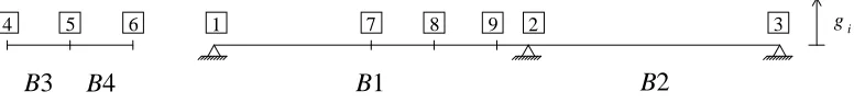
A simple example is used to introduce the types of degrees of freedom that are considered in the formulation of the vehicle-structure interaction in the context of a time step of the HHT method (see Figure 1). On the right, a simply supported beam with two spans (B1 and B2) is subjected to the contact of a vehicle, shown on the left. The structure of the vehicle is also composed of two beams (B3 and B4). Nodes 7, 8 and 9 are internal points of the beam B1. The location of these nodes may change between time steps, depending on the position of the vehicle. Eventual gaps between both structures (gi) can be easily considered in the
[image:4.595.101.489.490.537.2]compatibility equations, as will be shown later.
Figure 1. Vehicle and structure: beams and nodal points.
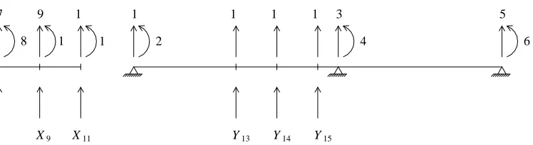
In each nodal point two degrees of freedom are considered (vertical displacement and rotation). Figure 2 shows the generalized displacements in nodal points (1 to 12), the generalized displacements of the contact points of the structure (13, 14 and 15), the interaction forces in the vehicle (X7, X9 and X11) and the interaction forces in the structure (Y13, Y14 and Y15). The interaction only involves the translational degrees of freedom.
1 7 8 9 2 3
6 5 4
B3
gi
Figure 2. Vehicle and structure: degrees of freedom and interactions forces.
The following classification of the degrees of freedom is considered: • F – free;
• X – interaction (vehicle); • P – prescribed;
• Y – interaction (structure).
This classification is used later in this section.
In the context of the HHT method, the dynamic equilibrium equation that involves the degrees of freedom in nodal points (1 to 12) is the following
(
)
c p(
)
c p(
)
c pc
F α F α u
K α u K α u
C α u C α u
M ɺɺ + 1+ ɺ − ɺ + 1+ − = 1+ − (1)
In this equation M is the mass matrix, C is the damping matrix, K is the stiffness matrix, F are the applied generalized forces, u are the generalized displacements and
α
is the main parameter of the HHT method. Whenα
= 0 the HHT method reduces to the Newmark method, and for other values of the parameterα
, numerical energy dissipation is introduced in the higher modes. The superscript c indicates the current time step ( t + ∆t ) and the superscript p indicates the previous one (t ).According to Figure 2 and to the classification indicated above, the F type degrees of freedom are the following: 2, 4, 6, 8, 10 and 12. The X type degrees of freedom correspond to the "supports" of the separated vehicle-structure, being the following: 7, 9 and 11. The P type degrees of freedom are the main structural supports 1, 3 and 5. The Y type degrees of freedom 13, 14 and 15 consist on the internal displacements of beam B1 at the contact points.
According to this classification of degrees of freedom, Eq. (1) can be expanded by considering several submatrices, yielding
7
8 9
1 1
1 1
2
3
4
5
6
1 1 1
Y 13 Y 14 Y 15
X 11
(
)
(
)
(
)
+ +
+ + −
+ +
+ + +
=
−
+ +
−
+ +
p P p Y PY p P
p X XX p X
p Y FY p F
c P c Y PY c P
c X XX c X
c Y FY c F
p P p X p F
PP PX PF
XP XX XF
FP FX FF
c P c X c F
PP PX PF
XP XX XF
FP FX FF
p P p X p F
PP PX PF
XP XX XF
FP FX FF
c P c X c F
PP PX PF
XP XX XF
FP FX FF
c P c X c F
PP PX
PF
XP XX
XF
FP FX
FF
R Y d P
X I P
Y d P α
R Y d P
X I P
Y d P α
u u u
K K K
K K K
K K K α
u u u
K K K
K K K
K K K α
u u u
C C C
C C C
C C C α
u u u
C C C
C C C
C C C α
u u u
M M
M
M M
M
M M
M
1 1
1
ɺ ɺ ɺ
ɺ ɺ ɺ
ɺ ɺ
ɺ ɺ
ɺ
ɺ (2)
In the F type degrees of freedom,
Y FY F
F P d Y
F = + (3)
being P the external loads applied in correspondence with each degree of freedom. Each component dij of dFY corresponds to the nodal force in the F type degree of freedom i, which is
equivalent to a single load consisting of a unitary value of Yj (see Figure 2).
In the X type degrees of freedom,
X XX X
X P I X
F = + (4)
being IXX the identity matrix with an appropriate size.
In the P type degrees of freedom,
P Y PY P
P P d Y R
F = + + (5)
being RP the reactions.
According to Figure 2, equilibrium equations in the contact degrees of freedom can be written, yielding
X
Y X
Y =− (6)
Since the number of Y type degrees of freedom coincides with the number of X type degrees of freedom, the subscript Y may be replaced with X.
(
)
(
)
(
)
(
)
(
)
− + + − − − − − + + − + = − + + − + + p P c P p X PX XX FX c X PX XX FX p P p X p F c P c X c F p P p X p F PP PX PF XP XX XF FP FX FF c P c X c F PP PX PF XP XX XF FP FX FF p P p X p F PP PX PF XP XX XF FP FX FF c P c X c F PP PX PF XP XX XF FP FX FF c P c X c F PP PX PF XP XX XF FP FX FF R α R α X d I d α X d I d α P P P α P P P α u u u K K K K K K K K K α u u u K K K K K K K K K α u u u C C C C C C C C C α u u u C C C C C C C C C α u u u M M M M M M M M M 0 0 0 0 1 1 1 1 1 ɺ ɺ ɺ ɺ ɺ ɺ ɺ ɺ ɺ ɺ ɺ ɺ (7)Eq. (7) is equivalent to the following three equations
(
)
(
)
(
)
(
)
(
)
(
)
(
)
(
)
pX FX c X FX p F c F p P FP p X FX p F FF c P FP c X FX c F FF p P FP p X FX p F FF c P FP c X FX c F FF c P FP c X FX c F FF X d α X d α P α P α u K α u K α u K α u K α u K α u K α u C α u C α u C α u C α u C α u C α u M u M u M + + − − + = − − − + + + + + + − − − + + + + + + + + 1 1 1 1 1 1 1 1 ɺ ɺ ɺ ɺ ɺ ɺ ɺ ɺ ɺ ɺ ɺ ɺ (8)
(
)
(
)
(
)
(
)
(
)
(
)
(
)
(
)
p(
)
(
)
(
)
(
)
(
)
(
)
(
)
(
)
(
)
pP c P p X PX c X PX p P c P p P PP p X PX p F PF c P PP c X PX c F PF p P PP p X PX p F PF c P PP c X PX c F PF c P PP c X PX c F PF R α R α X d α X d α P α P α u K α u K α u K α u K α u K α u K α u C α u C α u C α u C α u C α u C α u M u M u M − + + + + − − + = − − − + + + + + + − − − + + + + + + + + 1 1 1 1 1 1 1 1 1 ɺ ɺ ɺ ɺ ɺ ɺ ɺ ɺ ɺ ɺ ɺ ɺ (10)
By placing all terms containing unknown variables in the first member, Eq.s (8) and (9) result in
(
)
(
)
(
)
(
)
(
)
(
)
(
)
(
)
pP FP p X FX p F FF c P FP p P FP p X FX p F FF c P FP c P FP p X FX p F c F c X FX c X FX c F FF c X FX c F FF c X FX c F FF u K α u K α u K α u K α u C α u C α u C α u C α u M X d α P α P α X d α u K α u K α u C α u C α u M u M + + + + − + + + + − − + − + = + + + + + + + + + + + 1 1 1 1 1 1 1 1 ɺ ɺ ɺ ɺ ɺ ɺ ɺ ɺ ɺ ɺ ɺ ɺ (11)
(
)
(
)
(
)
(
)
(
)
(
)
(
)
(
)
pP XP p X XX p F XF c P XP p P XP p X XX p F XF c P XP c P XP p X XX p X c X c X XX c X XX c F XF c X XX c F XF c X XX c F XF u K α u K α u K α u K α u C α u C α u C α u C α u M X I α P α P α X I α u K α u K α u C α u C α u M u M + + + + − + + + + − − − − + = + − + + + + + + + + + 1 1 1 1 1 1 1 1 ɺ ɺ ɺ ɺ ɺ ɺ ɺ ɺ ɺ ɺ ɺ ɺ (12)
After the solution of the system of linear equations only the current reactions remain unknown. These can be calculated with the following equation
p P PP p X PX p F PF c P PP c X PX c F PF p P PP p X PX p F PF c P PP c X PX c F PF c P PP c X PX c F PF p X PX c X PX p P c P p P c P u K α α u K α α u K α α u K u K u K u C α α u C α α u C α α u C u C u C u M α u M α u M α X d α α X d P α α P R α α R + − + − + − + + + + − + − + − + + + + + + + + + + − + + + − + = 1 1 1 1 1 1 1 1 1 1 1 1 1 1 1 ɺ ɺ ɺ ɺ ɺ ɺ ɺ ɺ ɺ ɺ ɺ ɺ (13)
Eq. (11) can be written as
(
)
(
)
(
)
(
)
(
)
Fc X FX c
X FX c
F FF
c X FX c
F FF c
X FX c
F FF
F X d α u
K α u
K α
u C α u
C α u
M u M
= +
+ +
+ +
+
+ + +
+ +
1 1
1
1
1 ɺ ɺ
ɺ ɺ ɺ
ɺ (14)
being FF defined by
(
)
(
)
(
)
pP FP p
X FX p
F FF c
P FP
p P FP p
X FX p
F FF c
P FP
c P FP p X FX p
F c
F F
u K α u K α u K α u K α
u C α u C α u C α u C α
u M X d α P α P α F
+ +
+ +
−
+ +
+ +
−
− +
− +
=
1 1
1
ɺ ɺ
ɺ ɺ
ɺ
ɺ (15)
According to the Newmark method, the velocity and the displacement in the F type degrees of freedom, at the current time step (t + ∆t ), can be defined as [3]
( )
[
γ u γu]
tu
uɺFc = ɺFp + 1− ɺɺFp + ɺɺFc ∆ (16)
2 2
1
t u β u β t
u u
u Fc
p F p
F p F c
F ∆
+
− + ∆ +
= ɺ ɺɺ ɺɺ
(17)
These equations are also used in the HHT method. The parameter γ defines a linear weighting between the influence of the initial and final accelerations on the velocity variation and the parameter β defines a similar weighting of the accelerations on the displacement variation. These parameters influence the stability and accuracy of the HHT method.
Solving Eq. (17) for uɺɺFc gives
p F p
F p
F c
F c
F u
β u
t β u t β u t β
uɺɺ ɺ ɺɺ
− − ∆ − ∆ − ∆
= 1
2 1 1
1 1
2 2
(18)
Substituting uɺɺFc given by Eq. (18) into Eq. (16) yields
( )
u tβ u
t β u t β u t β γ t u γ u
u Fp
p F p
F c
F p
F p
F c
F ∆
− − ∆ − ∆
− ∆
+ ∆ −
+
= ɺ ɺɺ ɺ ɺɺ
ɺ 1
2 1 1
1 1
1 2 2
(19)
This equation can be rewritten as
+ − − ∆ +
− +
∆ − ∆
= γ
β γ γ t u β γ u
u t β
γ u t β
γ
u Fp
p F p F c
F c
F
2 1
1 ɺɺ
ɺ ɺ
p F p F p F c F c F u β γ t u β γ u t β γ u t β γ
uɺ ɺ ɺɺ
− ∆ + − + ∆ − ∆ = 2 1 1 (21)
By replacing F with X in Eq.s (16) and (17), and performing a similar rearrangement, one has, by analogy with Eq.s (18) and (21),
p X p X p X c X c X u β u t β u t β u t β
uɺɺ ɺ ɺɺ
− − ∆ − ∆ − ∆ = 1 2 1 1 1 1 2 2 (22) p X p X p X c X c X u β γ t u β γ u t β γ u t β γ
uɺ ɺ ɺɺ
− ∆ + − + ∆ − ∆ = 2 1 1 (23)
The substitution of Eq.s (18), (21), (22) and (23) into Eq. (14) yields
(
)
(
)
(
)
(
)
(
)
Fc X FX c X FX c F FF p X p X p X c X FX p F p F p F c F FF p X p X p X c X FX p F p F p F c F FF F X d α u K α u K α u β γ t u β γ u t β γ u t β γ C α u β γ t u β γ u t β γ u t β γ C α u β u t β u t β u t β M u β u t β u t β u t β M = + + + + + + − ∆ + − + ∆ − ∆ + + − ∆ + − + ∆ − ∆ + + − − ∆ − ∆ − ∆ + − − ∆ − ∆ − ∆ 1 1 1 2 1 1 1 2 1 1 1 1 2 1 1 1 1 1 2 1 1 1 1 2 2 2 2 ɺ ɺ ɺ ɺ ɺ ɺ ɺ ɺ ɺ ɺ ɺ ɺ (24)
(
)
(
)
(
)
(
)
(
)
(
)
(
)
− ∆ + − + ∆ + + − ∆ + − + ∆ + + − + ∆ + ∆ + − + ∆ + ∆ + = + + + + ∆ + + ∆ + + + ∆ + + ∆ p X p X p X FX p F p F p F FF p X p X p X FX p F p F p F FF F c X FX c X FX FX FX c F FF FF FF u β γ t u β γ u t β γ C α u β γ t u β γ u t β γ C α u β u t β u t β M u β u t β u t β M F X d α u K α t β γ C α M t β u K α t β γ C α M t β ɺ ɺ ɺ ɺ ɺ ɺ ɺ ɺ ɺ ɺ ɺ ɺ 1 2 1 1 1 2 1 1 1 2 1 1 1 1 2 1 1 1 1 1 1 1 1 1 1 2 2 2 2 (25)which is equivalent to the following compact form
(
)
Fc X FX c X FX c F
FFu K u α d X F
K + + 1+ = (26)
being
(
)
FF(
)
FFFF
FF A M α AC α K
K = 0 + 1+ 1 + 1+ (27)
(
)
FX(
)
FXFX
FX A M α AC α K
K = 0 + 1+ 1 + 1+
[
]
[
]
(
)
[
]
(
)
[
p]
X p X p X FX p F p F p F FF p X p X p X FX p F p F p F FF F F u A u A u A C α u A u A u A C α u A u A u A M u A u A u A M F F ɺ ɺ ɺ ɺ ɺ ɺ ɺ ɺ ɺ ɺ ɺ ɺ 5 4 1 5 4 1 3 2 0 3 2 0 1
1+ + + + + + +
+ + + + + + + = (28) 2 0 1 t β A ∆ = t β γ A ∆ = 1 t β A ∆ = 1 2 (29) 1 2 1 3= −
β
A 4 = −1
β γ A − ∆ = 1 2 5 β γ t A
(
)
(
)
(
)
(
)
(
)
Xc X XX c X XX c F XF c X XX c F XF c X XX c F XF F X I α u K α u K α u C α u C α u M u M = + − + + + + + + + + + 1 1 1 1
1 ɺ ɺ
ɺ ɺ ɺ
ɺ (30)
being FX defined by
(
)
(
)
(
)
pP XP p X XX p F XF c P XP p P XP p X XX p F XF c P XP c P XP p X XX p X c X X u K α u K α u K α u K α u C α u C α u C α u C α u M X I α P α P α F + + + + − + + + + − − − − + = 1 1 1 ɺ ɺ ɺ ɺ ɺ ɺ (31)
The substitution of Eq.s (18), (21), (22) and (23) into Eq. (30) yields
(
)
(
)
(
)
(
)
(
)
Xc X XX c X XX c F XF p X p X p X c X XX p F p F p F c F XF p X p X p X c X XX p F p F p F c F XF F X I α u K α u K α u β γ t u β γ u t β γ u t β γ C α u β γ t u β γ u t β γ u t β γ C α u β u t β u t β u t β M u β u t β u t β u t β M = + − + + + + − ∆ + − + ∆ − ∆ + + − ∆ + − + ∆ − ∆ + + − − ∆ − ∆ − ∆ + − − ∆ − ∆ − ∆ 1 1 1 2 1 1 1 2 1 1 1 1 2 1 1 1 1 1 2 1 1 1 1 2 2 2 2 ɺ ɺ ɺ ɺ ɺ ɺ ɺ ɺ ɺ ɺ ɺ ɺ (32)
(
)
(
)
(
)
(
)
(
)
(
)
(
)
− ∆ + − + ∆ + + − ∆ + − + ∆ + + − + ∆ + ∆ + − + ∆ + ∆ + = + − + + ∆ + + ∆ + + + ∆ + + ∆ p X p X p X XX p F p F p F XF p X p X p X XX p F p F p F XF X c X XX c X XX XX XX c F XF XF XF u β γ t u β γ u t β γ C α u β γ t u β γ u t β γ C α u β u t β u t β M u β u t β u t β M F X I α u K α t β γ C α M t β u K α t β γ C α M t β ɺ ɺ ɺ ɺ ɺ ɺ ɺ ɺ ɺ ɺ ɺ ɺ 1 2 1 1 1 2 1 1 1 2 1 1 1 1 2 1 1 1 1 1 1 1 1 1 1 2 2 2 2 (33)which is equivalent to the following compact form
(
)
Xc X XX c X XX c F
XFu K u α I X F
K + − 1+ = (34)
being
(
)
XF(
)
XFXF
XF A M α AC α K
K = 0 + 1+ 1 + 1+ (35)
(
)
XX(
)
XXXX
XX A M α AC α K
K = 0 + 1+ 1 + 1+
[
]
[
]
(
)
[
]
(
)
[
p]
X p X p X XX p F p F p F XF p X p X p X XX p F p F p F XF X X u A u A u A C α u A u A u A C α u A u A u A M u A u A u A M F F ɺ ɺ ɺ ɺ ɺ ɺ ɺ ɺ ɺ ɺ ɺ ɺ 5 4 1 5 4 1 3 2 0 3 2 0 1
1+ + + + + + +
+ + + + + + + = (36)
The parameters A0 to A5 are defined by Eq. (29). In matrix notation, Eq.s (26) and (34) become
corresponding displacement of the structure must be equal to the gap gi (see Figures 1 and 2).
This compatibility equation can be written as
c X c Y c
X u g
u − = (38)
being
c Y YY c P YP c F YF c
Y c u c u f Y
u = + + (39)
In this equation, each component cij of cYF corresponds to the displacement in the Y type
degree of freedom i for a single unit displacement in the F type degree of freedom j (see Figure 2). The components of matrix cYP have a similar meaning. Each component fij of fYY
corresponds to the displacement in the Y type degree of freedom i for a single load consisting of a unitary force on the Y type degree of freedom j (see Figure 2). All the components of the matrix fYY are calculated assuming null generalized displacements in the F type and P type
degrees of freedom. When the finite elements are based on the beam theory the fYY matrix is
not null. In finite elements whose formulation is based on shape functions the fYY matrix is
null.
Since the number of Y type degrees of freedom coincides with the number of X type degrees of freedom, the subscript Y may be replaced with X. Substituting Eq. (6) into Eq. (39), yields
c X XX c P XP c F XF c
Y c u c u f X
u = + − (40)
Substituting Eq. (40) into Eq. (38) gives
c P XP c X c X XX c X c F
XF u u f X g c u
c + + = +
− (41)
Multiplying both members of Eq. (41) by the constant −
(
1+α
)
results in(
)
(
)
(
)
(
)
(
)
cP XP c
X c
X XX c
X c
F
XF u α u α f X α g α c u
c
α − + − + =− + − +
+ 1 1 1 1
1 (42)
Rewriting Eq.s (37) and (42) in matrix form leads to
(
)
(
)
(
)
(
)
(
)
=
+ − +
− +
+ −
+
X X F
c X c X c F
XX XX
XF
XX XX
XF
FX FX
FF
g F F
X u u
f α I
α c
α
I α K
K
d α K
K
1 1
1
1
1 (43)
being
(
)
(
)
cP XP c
X
X α g α c u
[image:14.595.71.530.372.743.2]It is possible to demonstrate that in Eq. (43) the coefficient matrix of the system of linear equations is symmetric.
4. NUMERICAL EXAMPLE
In order to validate the proposed formulation, a simply supported beam subjected to a moving sprung mass is analyzed. This example is solved by the present direct method and by an iterative method proposed in [4] and [5]. The obtained results are also compared with those published in [6] and [7].
Figure 3 shows a simply supported beam subjected to a moving sprung mass. The properties of the simply supported beam coincide with those used by Yang and Wu [8], being the span L = 25.0 m and its geometrical and mechanical properties the following: Young’s modulus E = 2.87 GPa, Poisson’s ratio υ = 0.2, moment of inertia I = 2.90 m4 and mass per unit length m = 2303 kg/m. The beam is divided in 50 finite elements.
The sprung mass is modeled with two vertical beams. The upper beam simulates the mass Ms = 5750 kg and the lower beam simulates the stiffness k = 1595×103 N/m of the vehicle.
The constant velocity of the sprung mass is v = 100 km/h, its frequency is fv = 2.65 Hz and its
mass ratio Ms/(mL) is 0.1. The damping effects of the bridge and vehicle are considered to be
negligible.
In the numerical integration by the HHT method the following parameters are considered: ∆t = 0.005 s,
β
= 0.25,γ
= 0.50 andα
= 0. The total number of time steps is 180.MS k
v
[image:15.595.109.508.402.498.2]25.0
Figure 3. Simply supported beam subjected to a moving sprung mass.
-0.0025 -0.0020 -0.0015 -0.0010 -0.0005 0.0000 0.0005
0.0 0.1 0.2 0.3 0.4 0.5 0.6 0.7 0.8 0.9 Time (s)
M
id
p
o
in
t
d
ef
le
c
ti
o
n
(
m
)
Direct method without interaction Iterative method without interaction Direct method with interaction Iterative method with interaction
-0.40 -0.20 0.00 0.20 0.40 0.60 0.80
0.0 0.1 0.2 0.3 0.4 0.5 0.6 0.7 0.8 0.9 Time (s)
M
id
p
o
in
t
a
cc
el
er
a
ti
o
n
(
m
/s
2)
[image:16.595.74.525.99.229.2]Direct method without interaction Iterative method without interaction Direct method with interaction Iterative method with interaction
Figure 4. Vertical deflection and acceleration at the midpoint of the beam.
The sprung mass deflection and acceleration are plotted in Figure 5.
-0.0030 -0.0025 -0.0020 -0.0015 -0.0010 -0.0005 0.0000 0.0005
0.0 0.1 0.2 0.3 0.4 0.5 0.6 0.7 0.8 0.9
Time (s)
S
p
ru
n
g
m
a
ss
d
e
fl
e
ct
io
n
(
m
)
Direct method with interaction Iterative method with interaction
-0.20 -0.15 -0.10 -0.05 0.00 0.05 0.10 0.15 0.20 0.25 0.30
0.0 0.1 0.2 0.3 0.4 0.5 0.6 0.7 0.8 0.9 Time (s)
S
p
ru
n
g
m
a
ss
a
cc
el
er
a
ti
o
n
(
m
/s
2)
[image:16.595.75.530.291.423.2]Direct method with interaction Iterative method with interaction
Figure 5. Vertical deflection and acceleration of the sprung mass.
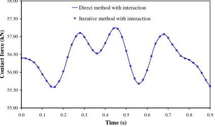
Figure 6 shows the variation of the contact force between the sprung mass and the simply supported beam.
55.00 55.50 56.00 56.50 57.00 57.50 58.00
0.0 0.1 0.2 0.3 0.4 0.5 0.6 0.7 0.8 0.9 Time (s)
C
o
n
ta
ct
f
o
rc
e
(k
N
)
Direct method with interaction Iterative method with interaction
Figure 6. Contact force between the sprung mass and the simply supported beam.
[image:16.595.201.413.496.622.2]5. CONCLUSIONS
In the present work an integrated model whose aim is the dynamic analysis of structures by the Hilber-Hughes-Taylor method is proposed. This algorithm treats the interaction between moving vehicles and a structure such as a bridge. This work provides a significant improvement relatively to the method proposed in [4] and [5], since the compatibility between vehicle and structure is no longer imposed by an iterative method, but by means of an integrated formulation that considers as variables displacements and contact forces. The governing system of equations comprises dynamic equilibrium equations and compatibility equations. The system of linear equations that arises at each time step is efficiently solved by Gaussian elimination, by considering several submatrices and their own characteristics. A significant improvement in terms of efficiency and precision could be observed.
ACKNOWLEDGMENTS
The authors wish to acknowledge the support provided by RAVE in the context of the protocol between RAVE and FEUP. This paper reports research developed under financial support provided by "FCT - Fundação para a Ciência e Tecnologia", Portugal.
REFERENCES
[1] A.F.M. Azevedo, J.A.O. Barros, J.M. Sena-Cruz and A. Ventura-Gouveia, “Software no ensino e no projecto de estruturas” (Educational software for the design of structures). In: Proceedings of the III Engineering Luso-Mozambican Congress, Maputo, Mozambique, pp. 81-92 (in Portuguese), (2003).
<http://civil.fe.up.pt/pub/people/alvaro/pdf/2003_Mocamb_Soft_Ens_Proj_Estrut.pdf>
[2] T.J.R. Hughes, “The Finite Element Method”, Dover Publications, Inc., New York, (2000).
[3] R. Clough and J. Penzien, "Dynamics of Structures", McGraw–Hill Book Company, New York, (1993).
[4] S. Cruz, “Dynamic behaviour of railway bridges in highspeed lines”, MSc Thesis, Faculty of Engineering of the University of Porto (in Portuguese), (1994).
[5] R. Calçada, “Dynamic effects on bridges due to highspeed railway traffic”, MSc Thesis, Faculty of Engineering of the University of Porto (in Portuguese), (1995). [6] R. Calçada and A. Cunha, “Stochastic modelling of the dynamic behaviour of bridges
under road traffic loads”, Computational Mechanics, New Trends and Applications, E. Onate and S.R. Idelsohn (Eds.), CIMNE, Barcelona, Spain (1998).
[7] C.J. Bowe and T.P. Mullarkey, “Wheel-rail contact elements incorporating irregularities”, Advances in Engineering Software Vol. 36, pp. 827-837, (2005).