Automatic Detection of Whitefly Pest using Statistical Feature Extraction and Image Classification Methods

© 2016, IRJET | Impact Factor value: 4.45 | ISO 9001:2008 Certified Journal | Page 950

Automatic Detection of Whitefly Pest using Statistical Feature

Extraction and Image Classification Methods

Abhishek Dey

_{, Debasmita Bhoumik}

_{, Kashi Nath Dey}

1

Assistant Professor,

_{Department of Computer Science, Bethune College, West Bengal, India}

2

_{M.Tech. student, Department of Computer Science and Engineering, University of Calcutta, West Bengal, India}

3

_{Associate Professor, Department of Computer Science and Engineering, University of Calcutta, West Bengal, India}

---***---Abstract -

production of good quality food, improved quality of life and a stable agricultural economy. Excessive use of pesticides for pest control is harmful to plants, animals as well as human beings. Digital image processing along with computer vision techniques can be applied for early detection of pests and it can minimize amount of pesticides used in the plants. Generally, leaves are the most affected part of the plants. So, the study of interest is the leaf, rather than whole plant. Among many pests, the white fly is one of the most hazardous pests that affect the leaves. This paper presents an automated approach for detection of white fly pest from leaf images of various plants. Initially, image pre-processing techniques such as noise removal and contrast enhancement are used for improving the quality of image thus making it suitable for further processing. Then, k-means clustering method is used for segmenting pest from infected leaves. After that, texture features are extracted from those segmented images by statistical feature extraction methods such as Gray Level Run Length Matrix (GLRLM) and Gray Level Co-occurrence Matrix (GLCM). Finally, various classifiers like Support Vector machine, Artificial Neural Network, Bayesian classifier, Binary decision tree classifier and k-Nearest neighbor classifier are used to distinguish between healthy leaf images from white fly pest infected leaf images.

Key Words: k-means clustering, Statistical feature extraction , Support Vector machine, Artificial Neural Network, Bayesian classifier, Binary decision tree classifier, K-nearest neighbor classifier

1. INTRODUCTION

Agriculture is the foundation of Indian economy as over 75% of its population is directly or indirectly engaged in this profession. Beyond the traditional agriculture, new trends in cropping pattern have been recognized for changing the status of rural community [1]_{. Due to the}

increase in demand in the agricultural industry, the need to effectively grow a plant and increase its yield is very important. In order to do so, it is important to monitor the plant during its growth period, as well as the time of harvest. The main source for the disease is the leaf. About 80% to

90% of disease on the plant is on its leaves. So, our study of interest is the leaf of the tree rather than whole plant. There are so many things that can cause different diseases to the plants among which pests are of utmost importance. A pest is any living organism which is harmful to plants. Pests can damage large crop fields. This results in decreased productivity of crops and ultimately the economy of the country is severely affected. If harmful pests are detected on the early basis and prevented accordingly, then big losses can be avoided. Pesticides can be used to control pests but they can be harmful to plants and humans if used uncontrollably and in excessive amount. To save time, efforts, labors and use of heavy pesticides there is a need of fast and accurate pest detection [2] _{. Among many pests,}

white fly is a very common which affects mainly leaves of cotton, bamboo, avocado, citrus etc. Whiteflies are soft-bodied, winged insects closely related to aphids. They can be found in any region, but they are so tiny that they are usually camouflaged. They can be as small as 1/12 of an inch, and are often found in clusters on the undersides of leaves [3]_{. In}

© 2016, IRJET | Impact Factor value: 4.45 | ISO 9001:2008 Certified Journal | Page 951

Specificity, Positive Predictive Accuracy (PPA) and Negative Predictive Accuracy (NPA). The rest of the paper is organized as follows. Section 2 describes some works related to pest detection in recent years. Section 3 elaborates the proposed methodology that includes image pre-processing techniques, texture feature extraction using statistical methods and classification using above mentioned five classifiers. Experimental results are shown in section 4. Finally, the conclusion is summarized in section 5.

2. LITERATURE REVIEW

Several studies are reported in literature for detection and classification of leaf pests.

In the year 2011, H. Al-Hiary, S. Bani-Ahmad, M.Reyalat, M.Braik & Z.AlRahamneh performed a work “Fast and Accurate Detection and Classification of Plant Diseases”

[4]_{. Here, automatic detection and classification of the plant}

diseases have been implemented using k-means segmentation algorithm followed by feature extraction using color co-occurrence method and classification using Artificial Neural Networks.

In the year 2011, Y. Tian, L. Wang and Q. Zhou performed a work “Grading method of Crop disease based on Image Processing” [5]_{. In this paper, a technique has been}

proposed where expanse and grading time is reduced as compared to manual system. The proposed methods follow three steps: preprocessing of image followed by segmentation and statistical analysis.

In the year 2013, F. Fina, P. Birch, R. Young, J. Obu, B. Faithpraise and C. Chatwin performed a work “Automatic Plant Pest detection and recognition using k-means clustering algorithm and correspondence filters” [6]. _{In this}

paper, testing is done using 10 different pests. The process of pest’s segmentation was started by identifying green colored pixels depending upon different threshold values. In the Second phase of algorithm angle multiplexing was done for those pests that had been detected with the help of k-means clustering algorithm.

In the year 2013 He, Qinghai performed a work "Cotton pests and diseases detection based on image processing." [7]_{. Damage ratio of cotton leaf caused by the}

pests is determined in this paper by using image enhancement and filtering algorithms. Comparisons of different color models like RGB, HSI and YCbCr has also been done by the authors.

In the year 2015, Mainkar, Prakash M., Shreekant Ghorpade, and Mayur Adawadkar performed a work "Plant Leaf Disease Detection and Classification Using Image Processing Techniques” [8]_{. In this paper, automated}

detection and classification of plant leaf diseases are implemented by several steps viz. image acquisition and pre-processing, k-means clustering based segmentation, GLCM features extraction and neural network based classification. In the year 2015, Warne, Pawan P., and S. R. Ganorkar performed a work "Detection of Diseases on Cotton Leaves Using K-Mean Clustering Method" [9]. _{In this}

paper, initially contrast enhancement of the input image is done by histogram equalization, K Means clustering algorithm is used for segmentation and finally classification is performed using neural network.

In the year 2016, Patil, Rupali performed a work “Grape Leaf Disease Detection Using k-means clustering Algorithm" [10]_{. The proposed algorithm is tested on five}

different diseases of the plant. After color preprocessing, the segmentation is done by using k-means clustering technique. In the next step, for each pixel map of the image for only HIS images the SGDM matrices were generated. Finally the extracted feature was recognized.

3. PROPOSED METHODOLOGY

© 2016, IRJET | Impact Factor value: 4.45 | ISO 9001:2008 Certified Journal | Page 952

Fig- 1: Block diagram of the proposed methodology

3.1

Image Preprocessing

The principal objective of pre-processing is to perform some basic tasks on a given image so that the resultant image is more suitable than the original image for subsequent image processing methods like segmentation, feature extraction and disease detection. Pre-processing eliminates disease independent variations from the input image, enhances some features of image or prevents undesired distortions. It doesn't increase the inherent information content of the data. Therefore, pre-processed images are more useful than original raw input images for computer vision and machine learning applications [11]_{. In}

our proposed method, the following pre-processing tasks are required to be done on the input leaf images for improving image quality:

Noise removal: Image noise is random variation of

brightness or color information in images, and is usually an aspect of electronic noise. It can be produced by the sensor and circuitry of a scanner or digital camera. Our goal is to remove the noise from the image in such a way that the original image is discernible. We have used two -dimensional Gaussian Filter with sigma =1 for noise removal. A Gaussian filter smooths an image by calculating weighted averages in a filter box [12]_{. It is more effective in smoothing images than}

normal mean filter.

Improvement of image contrast: After noise

removal, unsharp masking technique is used for improving image contrast. It returns an enhanced version of the grayscale or truecolor (RGB) input image where the image features, such as edges, have been sharpened. Sharpness is actually the contrast between different colors. Sharpening

images increases the contrast along the edges where different colors meet. The unsharp masking technique sharpens an image by subtracting a blurred (unsharp) version of the image from itself.

Fig- 2: (a) Input leaf image before pre-processing, (b) Leaf image after noise removal, (c) Leaf image after contrast enhancement

3.2 Segmentation

In computer vision, image segmentation is the process where a digital image is partitioned into multiple segments. A segment is basically a set of pixels, also called super pixel. Segmentation aims to simplify and change the representation of an image such that it becomes more meaningful and easier to analyze. It is typically used to locate objects and boundaries in images [13]_{. More precisely, image}

segmentation is the method of assigning a label to every pixel in an image such that same labeled pixels share certain characteristics. Image segmentation results in a set of segments that collectively cover the whole image or a set of contours extracted from the image. Each pixel in a region is similar with respect to some property like texture, intensity or color. Adjacent regions are significantly different with respect to the same characteristic(s). In this paper, we have used the original k-means clustering algorithm with some modification for segmenting the pest infected cluster.

© 2016, IRJET | Impact Factor value: 4.45 | ISO 9001:2008 Certified Journal | Page 953

mean, serving as a prototype of the cluster. Given a set of observations (x1, x2… xn), where each observation is a

d-dimensional real vector, k-means clustering aims to partition the n observations into k (≤ n) sets S = {S1, S2, …, Sk} so as to

minimize the within-cluster sum of squares (WCSS) (sum of distance functions of each point in the cluster to the K center). In other words, its objective is to find:

Here μi is the mean of

points in Si [14]

The main steps of k-means segmentation algorithm used in this paper are shown below:

Step 1: Read input image.

Step 2: Transform image from RGB to L*a*b* color space. Step 3: Classify colors using k-means clustering in ‘a*b*’ space.

Step 4: Label each pixel in the image from the results of K-Means.

Step 5: Generate images that segment the image by color. Step 6: Select disease containing segment.

From repeated observations, we have found that the cluster number that contains white fly pest changes each time after segmentation. Therefore, it became hard to choose the cluster which has to be checked further. From experiments we have concluded that the cluster which has the minimum- mean value contains white fly. Therefore, each time after segmentation the cluster with the minimum- mean value is found and saved for next phase feature extraction.

For the image in Figure 3: (a), after segmentation, cluster 1 of Figure 3: (c) has the minimum- mean value among all four clusters and therefore, it is to be saved for subsequent steps.

Fig-3: Result of applying k-means segmentation on a

whitefly affected leaf image. (a) Leaf image after pre-processing, (b) Leaf image labelled by cluster index (c) 1st

cluster, (d) 2nd _{cluster, (e) 3}rd _{cluster, (f) 4}th _cluster

3.3 Feature Extraction

The objective of feature extraction is to reduce the original data by measuring positive properties, or features that discriminate one input sample from another sample. It starts from an initial set of measured data and builds derived values (features) intended to be informative and non-redundant, facilitating the subsequent learning steps, and in some cases leading to better human interpretations. The texture of images refers to the appearance, structure and arrangement of the parts of an object within the image [15]_.

Though there is no strict definition of the image texture, it is easily perceived by humans and is considered to be a rich source of visual information about the nature and three dimensional shapes of physical objects [16]_{. In this paper,}

after segmentation process, all the images are converted to grayscale as Gray Level Co-occurrence Matrix (GLCM) and Gray Level Run Length Matrix (GLRLM) method only work on grayscale images. 16 texture features are extracted from pre-processed input images by using statistical methods as explained in the remaining part of this section. Entropy is extracted directly from greyscale images. It is defined as,

(1)

Entropy gives a statistical measure of randomness that can be used to characterize the texture of the input image, where p contains the histogram counts of the image [17]_.

© 2016, IRJET | Impact Factor value: 4.45 | ISO 9001:2008 Certified Journal | Page 954

count is then made of the number of pairs of pixels that possess a given distribution of grey-level values [18]_.

Formally, the G × G Gray Level Co-occurrence Matrix P for a displacement vector d = (dx, dy) is defined as follows. The entry (i, j) of P is the number of occurrences of the pair of gray levels i and j which are at distance d apart. Formally, P(i, j) = {((r, s), (t, v)): I(r,s)=i, I(t,v)=j | (r, s), (t, v) ∈ N × N, (t, v) = (r + dx, s + dy) }.

After creating GLCM of a pre-processed input image, we have used d = 1 and θ = 0o _{for extracting following four}

features from the matrix:-

Contrast: measuring of the intensity contrast between a pixel and its neighbor over the whole image. It is 0 for a constant image. (2)

Correlation: measuring how a pixel is

correlated to its neighbor over the whole image, where denotes mean values of i and j respectively and denotes standard deviations of i and j respectively. Correlation is 1 or -1 for a perfectly positively or negatively

correlated image. Correlation is NaN for a constant image. (3)

Energy: measuring sum of squared elements in

the GLCM. Energy is 1 for a constant image. (4)

Homogeneity: , measuring the closeness of the

distribution of elements in the GLCM to the GLCM diagonal.

Homogeneity is 1 for a diagonal GLCM. (5)

Run-length statistics capture the coarseness of a texture in specified directions. A run is defined as a string of consecutive pixels which have the same gray level intensity along a specific linear orientation. Fine textures tend to contain more short runs with similar gray level intensities, while coarse textures have more long runs with significantly different gray level intensities. This method allows extracting the higher order statistical texture features.

In run length matrix Pθ(i, j), each cell in the matrix

consists of the number of elements where gray level i successively appears j times in the direction θ. j is termed as run length [19]_{. The resultant matrix characterizes gray-level}

runs by the gray tone, length and the direction of the run. This method allows extracting the higher order statistical texture features. Texture properties obtained from GLRLM include the following five main features:-

Short Run Emphasis (SRE): , measuring fine texture

(6)

Long Run Emphasis (LRE): , measuring coarse

texture (7)

Run Length Non-uniformity (RLN): , measuring

similarity of run lengths (8)

Gray-Level Non-uniformity (GLN): measuring

similarity of gray level values (9)

Run Percentage (RP): , measuring the number of short runs, A is the area of interset in the image (10)

These 5 features along with 6 more features such as Low gray-level run emphasis (LGRE), High gray-level run emphasis (HGRE), Short run low gray-level emphasis (SRLGE), Short run high gray-level emphasis (SRHGE), Long run low gray-level emphasis (LRLGE) and Long run high gray-level emphasis (LRHGE) are extracted from horizontal direction (θ = 0o_{) of GLRLM of pre-processed images.}

3.4 Classification

In computer vision and machine learning, classification is the problem of identifying in which set of categories a new observation belongs, on the basis of a training set of data containing observations (or instances) whose category membership is already known. A classification task usually involves separating data into training and testing sets. Each instance in the training set contains one target value (i.e. the class labels) and several attributes (i.e. the features). There are various approaches for image classification.

We have used five different classifiers i.e. Support Vector machine (SVM), Artificial Neural Network (ANN), Bayesian classifier, Binary decision tree classifier and k-Nearest Neighbor (k-NN) classifier to classify white fly affected leaf images from normal leaf images.

3.4.1 Support Vector Machine (SVM)

© 2016, IRJET | Impact Factor value: 4.45 | ISO 9001:2008 Certified Journal | Page 955

{-1,+1}, the class label, with i=1..n. SVM finds the optimal separating hyper planes based on a kernel function (K). All images, of which feature vector lies on one side of the hyper plane, belong to class -1 and the others are belong to class +1. Simplest type of SVM is linear SVM, in which the training patterns are linearly separable. A linear function of this form is shown below:

f(x) = wT _{x + b (11)}

such that for each training sample xi the function yields f(xi)>

0 for yi = +1, and f(xi) < 0 for yi = -1. In other words, training

samples of two different classes are separated by the hyperplane f(x) = wT _{x + b = 0, where w is weight vector and}

normal to hyperplane, b is bias or threshold and xi is the data point.

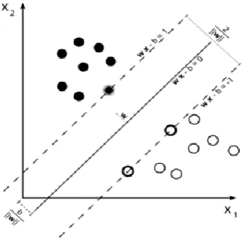
Fig-4: Maximum-margin hyper plane and margins for a

linear SVM trained with samples from two classes

In Figure 4, white and black circles indicate data points of two different classes separated by a hyperplane that minimizes the separating margin between the two classes which is obtained by using linear SVM. Support vectors are elements of the training set that lie on the boundary hyperplane of the two classes.

Fig-5: Non-linear SVM classification

If the data of the classes cannot be separated, then the non-linear SVM classifier is used. In a nonlinear SVM classifier, a nonlinear operator is used to map the input pattern x into a higher dimensional space H as shown in Figure 5. The nonlinear SVM classifier is defined as, f(x) = wT _{ϕ(x) + b (12)}

The transformation from non-linear to linear separating hyperplane in higher dimensional feature space is done by taking help of kernel functions [20]_{. A kernel function on two}

samples, represented as feature vectors in some input space, is defined as k(xi, xj) = ϕ(xi)T ϕ(xj), ϕ is the feature vector.

Most commonly used kernels are:

Linear kernel: k(xi, xj) = xiTxj (13)

Polynomial Kernel: k(xi, xj) = (γxiTxj + r)d, γ>0 (14)

RBF Kernel: k(xi, xj) = , σ>0 (15)

Sigmoid Kernel: k(xi, xj) = tanh(γxiTxj + r) (16)

3.4.2 Artificial Neural Network (ANN)

In machine learning, ANNs are a family of models inspired by biological neural networks which are used to estimate or approximate functions that can depend on a large number of inputs and are generally unknown. In this paper, a Pattern Recognition Neural Network is used for classification [21]_{. It is a feedforward network with the default}

tan-sigmoid transfer function in the hidden layer, and a softmax transfer function in the output layer. In this technique, the entire data set is divided into three subsets. The first subset is the training set that is used for computing the gradient and updating the network weights and biases. The second subset is the validation set. The error on the validation set is monitored during the training process. The validation error normally decreases during the initial phase of training, as does the training set error. However, when the network begins to overfit the data, the error on the validation set generally begins to rise. The network weights and biases are saved at the minimum of the validation set error. The test set is not used during training, it is only used for testing the trained network on unknown data. Number of hidden layers has to be fixed also to gain efficiency in classification [22]_{. Neural networks are adjusted or trained so}

© 2016, IRJET | Impact Factor value: 4.45 | ISO 9001:2008 Certified Journal | Page 956

3.4.3 Bayesian Classifier

The naive Bayes classifier uses Bayes theorem and assumes that the predictors are conditionally independent of one another within each class. Though the assumption is sometimes violated in practical cases, naive Bayes classifiers tend to yield posterior distributions that are robust to biased class density estimates, particularly where the posterior is 0.5 (the decision boundary) [23] _.

Using this algorithm the classification is done in following steps:

1. The densities of the predictors are estimated within each class.

2. Posterior probabilities are modeled according to Bayes rule. That is, for all k = 1,...,K,

(17)

Where, Y is the random variable corresponding to the class index of an observation, X1,...,XP are the random predictors of

an observation, Π(Y=k) is the prior probability that a class index is k.

3. An observation is classified by estimating the posterior probability for each class, and the observation is then assigned to the class yielding the maximum posterior probability.

3.4.4 Binary Decision Tree Classifier

In a decision tree, each internal node is associated with a decision and leaf nodes are associated with response or class label. Each internal node tests one or more attribute values leading to two or more outgoing edges. Each edge in turn is associated with a possible value of the decision. These edges are mutually distinct and collectively exhaustive; there is an edge for every possibility. In case of a binary decision tree, there are two outgoing edges from each internal node. One edge represents the outcome “yes” or true and for the other edge “no” or “false”. Therefore, an outcome using decision tree is obtained by following the decisions in the tree from

the root node down to a leaf node. In this paper, binary classification decision tree is used for classification purpose

[24]_.

3.4.5 k- Nearest Neighbor Classifier (k-NN)

In pattern recognition, k-NN algorithm is a non-parametric method used for classification. The input consists of the k closest training examples in the feature space and the output is a class membership. An object is classified by a majority vote of its neighbors, with the object being assigned to the class most common among its k nearest neighbors (k is a positive integer, typically small). If k = 1, then the object is simply assigned to the class of that single nearest neighbor. Value of k is crucial for obtaining good accuracy

[25].

4. EXPERIMENTAL RESULT AND DISCUSSION

All the image pre-processing, segmentation, feature extraction and classification techniques in our proposed method are simulated in MATLAB 8.5 (R2015a) and run on an Intel(R) Core(TM) with 4-GB memory. We have obtained leaf images (both normal and pest affected) from few authenticated image databases such as http://www.ipmimages.org/ and http://www.bugwood.org/ImageArchives.html. 200 such images are used as input to our proposed system. This set of 200 images contains 125 affected and 75 normal images. For training we have used 70 images among them 40 affected and 30 normal. For testing there are 130 images among them 85 affected and 45 normal. After pre-processing and segmentation steps, 16 texture features are extracted from from these images as described in section 3.3.

© 2016, IRJET | Impact Factor value: 4.45 | ISO 9001:2008 Certified Journal | Page 957

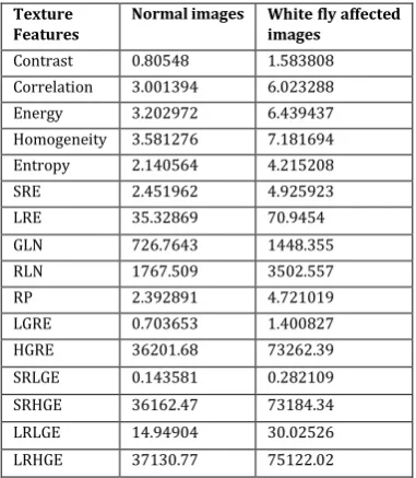
Table 1: Comparison of feature values of normal and

affected leaf images

Texture Features

Normal images White fly affected images

Contrast 0.80548 1.583808

Correlation 3.001394 6.023288

Energy 3.202972 6.439437

Homogeneity 3.581276 7.181694

Entropy 2.140564 4.215208

SRE 2.451962 4.925923

LRE 35.32869 70.9454

GLN 726.7643 1448.355

RLN 1767.509 3502.557

RP 2.392891 4.721019

LGRE 0.703653 1.400827

HGRE 36201.68 73262.39

SRLGE 0.143581 0.282109

SRHGE 36162.47 73184.34

LRLGE 14.94904 30.02526

LRHGE 37130.77 75122.02

It can be observed that for all of the 16 features, average feature values of the affected leaves are greater than that of the normal leaves. This is because the white fly affected leaf images have more random texture than normal leaf images due to presence of pest. Then this feature matrix is fed into the previously mentioned 5 classifiers at section 3.4.

Performance of all the classifiers can be tested and evaluated by the following parameters:

Accuracy rate = Correctly classified images / Classified images

Sensitivity = Correctly classified positive images / True positive images

Specificity = Correctly classified negative images / True negative images

Positive Predictive Accuracy (PPA) = Correctly classified positive images / Positive classified images

Negative Predictive Accuracy (NPA) = Correctly classified negative images / Negative classified images

In our work, SVM classifier is trained using different kernel functions. From experiment, it is observed that using Radial Basis Function (RBF) kernel, SVM classifier can achieve highest accuracy of 100% after training. So, we have used the cross-validated trained classifier using RBF kernel for further testing on new images. Performance testing of all the 5 trained classifier is done on 130 test images (45 normal and 85 affected) which were not in the set of input images used for training.

Table 2:Performance Comparison of Different Classifiers

Now we plot the performance metrics of those 5 classifiers in the graph of figure 6 and compare their outcome.

Fig 7: Graphical view of comparison of performance metrics

Hence, analyzing the obtained results from Table 2 and Figure 7 demonstrates that SVM gives highest Accuracy, Sensitivity, Specificity, PPA and NPA for separating white fly pest infected leaf images from normal leaf images

.

5. CONCLUSION

It is well known that white fly is a vulnerable pest which can affect a variety of plants and crops. In this paper, an automated system is developed for separating white fly pest infected leaf images from normal leaf images. Popular classification methods are used and a detailed comparison of their performances is studied. Among all the classifiers, the computational efficiency of SVM is great as it needs only a few minutes of runtime for training and also a small training set is needed to provide very good results because only the support vectors are of importance during training. For these reasons, SVM tends to perform better than other methods. Applying this trained SVM classifier on a new set of test images, we have obtained accuracy of 98.46%. Hence, it can be concluded that our proposed method is very much efficient for automated detection of white fly from leaf images and also computationally very fast. This method is

Classifier Accuracy Sensitivity Specificity PPA NPA

SVM 98.46% 98.82% 97.78% 98.82% 97.78%

ANN 90% 93.9% 83.33% 90.59% 88.89%

Bayesian 93.85% 98.73% 86.27% 91.76% 97.78%

Binary Decision Tree

90% 93.9% 83.33% 90.59% 88.89%

© 2016, IRJET | Impact Factor value: 4.45 | ISO 9001:2008 Certified Journal | Page 958

them from the burden of time consuming manual checking of leaf and to increase productivity by earlier detection of infected leaves

REFERENCES

[1] Pandey, Rashmi, Sapan Naik, and Roma Marfatia. "„Image Processing and Machine Learning for Automated Fruit Grading System: A Technical Review”." International Journal of Computer Applications 81.16 (2013).

[2] Masood, Rabia, S. A. Khan, and M. N. A. Khan. "Plants Disease Segmentation using Image Processing." International Journal of Modern Education & Computer Science 8.1 (2016).

[3] groggsgreenbarn.com. 2016. common- garden-pests. [ONLINE] Available at: http://groggsgreenbarn.com/common-garden-pests. [Accessed 1 August 2016].

[4] H.Al-Hiary, S. Bani-Ahmad, M.Reyalat, M.Braik & Z.AlRahamneh, “Fast and Accurate Detection and Classification of Plant Diseases”, International Journal of Computer Applications, Vol. 17, No.1, pp. 31-38.March 2011

[5] Y. Tian, L. Wang and Q. Zhou, “Grading method of Crop disease based on Image Processing”, Computer and computing technologies in agriculture 427-433, 2011.

[6] F. Fina, P. Birch, R. Young, J. Obu, B. Faithpraise and C. Chatwin, “Automatic Plant Pest detection and recognition using k-meansclustering algorithm and correspondence filters”, International Journal of Advanced Biotechnology and Research, Vol. 4, Issue 2, pp 189-199, 2013.

[7] He, Qinghai, et al. "Cotton pests and diseases detection based on image processing." Telkomnika Indonesian Journal of Electrical Engineering 11.6 (2013): 3445-3450.

[8] Mainkar, Prakash M., Shreekant Ghorpade, and Mayur Adawadkar. "Plant Leaf Disease Detection and Classification Using Image Processing Techniques." International Journal of Innovative and Emerging Research in Engineering 2.4 (2015). [9] Warne, Pawan P., and S. R. Ganorkar. "Detection of Diseases on Cotton Leaves Using K-Mean Clustering Method." (2015).

[10] Patil, Rupali, et al. "Grape Leaf Disease Detection Using K-meansClustering Algorithm." (2016).

[11] Mrs.S.Rathinam, Dr.S.Selvarajan; “ Comparison of Image Preprocessing Techniques on Fundus Images for Early Diagnosis of Glaucoma”; International Journal of Scientific & Engineering Research, Volume 4, Issue 12, December-2013

[12] S.Sri Abirami, S.J Grace Shoba; “Glaucoma Images Classification Using Fuzzy Min-Max Neural Network Based On Data-Core”; International Journal of Science and Modern Engineering (IJISME), ISSN: 2319-6386, Volume-1, Issue-7, June 2013

[13] Kumar, Satish, and Raghavendra Srinivas. "A Study on Image Segmentation and its Methods." International Journal of Advanced Research in Computer Science and Software Engineering 3.9 (2013).

[14] Dubey, Shiv Ram, and Anand Singh Jalal. "Adapted approach for fruit disease identification using images." preprintarXiv:1405.4930 (2014).

[15] G. Castellano, L. Bonilha, L.M. Li, F. Cendes; “Texture analysis of medical images”; Clinical radiology 59 (12), 2004, pp. 1061-1069

[16] Manoj kumar M, Manu A.R; “A Study On Texture Feature Analysis And Effect Of Window Size On Texture”; Journal of Research in Electrical and Electronics Engineering (ISTP-JREEE), Volume 2, Issue 1, Jan. 2013, pp. 6-13

[17] Hari Babu Nandpuru, Dr. S. S. Salankar, Prof. V. R. Bora; “IEEE Students' Conference on Electrical, Electronics and Computer Science”; 2014, pp. 1-6

[18] Alaa Eleyan, Hasan Demirel; “Co-occurrence matrix and its statistical features as a new approach for face recognition”; Turk J Elec Eng & Comp Sci, Vol.19, No.1, 2011, pp. 97-107

[19] Lee You Tai Danny, Dr. Rajendra Acharya Udyavara; “COMPUTER BASED DIAGNOSIS OF GLAUCOMA USING PRINCIPAL COMPONENT ANALYSIS (PCA): A COMPARATIVE STUDY”; SIM university, 2011

© 2016, IRJET | Impact Factor value: 4.45 | ISO 9001:2008 Certified Journal | Page 959

"Review and comparison of methods to study the contribution of variables in artificial neural network models." Ecological modelling 160.3 (2003): 249-264.

[22] Gardner, G. G., et al. "Automatic detection of diabetic retinopathy using an artificial neural network: a screening tool." British journal of Ophthalmology 80.11 (1996): 940-944.

[23] Rish, Irina. "An empirical study of the naive Bayes classifier." IJCAI 2001 workshop on empirical methods in artificial intelligence. Vol. 3. No. 22. IBM New York, 2001.

[24] Safavian, S. Rasoul, and David Landgrebe. "A survey of decision tree classifier methodology." (1990).

[25] Li, Leping, et al. "Gene selection for sample classification based on gene expression data: study of sensitivity to choice of parameters of the GA/KNN method." Bioinformatics 17.12 (2001): 1131-1142.

BIOGRAPHIES

Abhishek Dey, an Assistant Professor in Computer Science in Bethune College, Kolkata, India. His research interests are in Image Processing, Machine learning, Artificial

Intelligence and Computer Vision.

Debasmita Bhoumik,a student of Master of Technology, Department of Computer Science and Engineering, in University of Calcutta, Kolkata, India. Her research interests are in Image Processing and Machine learning.