Tuning controller parameters and load frequency control of multi area multi source power system by Particle Swarm Optimization Technique

(1)

Page 863

Tuning controller parameters and load frequency control of multi-area

multi-source power system by Particle Swarm Optimization Technique

V.Jyothi

1

_{, P. Bharat Kumar}

2

1

_{PG Scholar, Department of EEE, JNTU Anantapur, Andhra Pradesh, India}

2

_{Lecturer, Department of EEE, JNTU Anantapur, Andhra Pradesh, India}

---

Abstract-

This article presents the setting of the controller parameters using particle swarm optimization (PSO) and its application to the load frequency control (LFC) of a power system from several sources that have different production sources as hydropower, thermal and gas power plants. A controller (PID) proportional integral derivative is used for tuning and analysis of the proposed model. The optimization of particle swarm algorithm (PSO) has been developed for the appropriate control settings for optimal performance. The superiority of the proposed approach was demonstrated by comparing the results with the optimum output feedback controller algorithm used for the same power systems. The comparison is made through various performance measures such as excess, time and standard error criteria of power frequency and tie-line after a disturbance step (SLP) load pertubation. Note that the dynamic performance of the proposed controller is improved by using PSO. Further-more, it also notes that the proposed system is robust and unaffected by the change of the charge state, the parameters of the system and the size of SLP.

1. INTRODUCTION:

The problem of controlling the actual output power generating units in response to changes in the frequency of the exchange system and tie-line power within specified

limits is known as load frequency control (LFC).In general,

it is considered as a part of automatic generation control (AGC) and is very important in the operation and control

of power systems.Energy systems on a large scale usually

consist of control zones or regions that represent coherent

groups of generators. The control area may have a

combination of thermal, hydro, gas, nuclear and renewable

sources of energy. Researchers around the world are

trying to propose several strategies for LFC power systems in order to maintain the system frequency and tie line flow in their programmed values during normal operation and

during small perturbations.Paper is literature that most of

the works of LFC were carried out in two hydrothermal

systems or thermal-thermal areas. It is noted that

considerable research will propose best AGC systems based on modern control theory, neural networks, fuzzy systems theory, reinforcement learning [8] and ANFIS

approach.But these advanced approaches are complicated

and require familiarity of users to these techniques, thus

reducing its applicability. Alternatively, classic controllers

Proportional Integral Derivative (PID) remain the preferred choice of an engineer because of its structural simplicity, reliability and favorable relationship between

performance and cost.It also offers the simplified dynamic

modeling, requiring less user skills, and minimal development effort, which are the main problems of

engineering practice. The growth in the size and

complexity of power systems with increased energy demand has necessitated the use of intelligent systems that combine knowledge, techniques and methodologies from various sources for real-time control of energy

systems.

The burden of a power system is constant and never given to ensure the quality of energy supply, a frequency controller load is needed to maintain the system frequency

to the desired nominal value. In an energy system

deregulated, each control area contains different types of uncertainties and various disturbances due to more complex modeling errors of the system and change the structure of power system Therefore, a control strategy need not only maintains the constancy of the flow rate and tie-desired power but also achieves zero steady-state error

and inadvertent exchange.

The controller proportional integral derivative (PID) is the most popular feedback controller used in the process

industries.It is a robust controller, easy to understand that

it can provide excellent control performance despite the

various dynamic characteristics of the process plant. As

the name suggests, the PID algorithm has three basic modes, proportional mode, integral and derivative modes. A proportional controller has the effect of reducing the rise

time but never eliminates steady state error. An integral

(2)

Page 864

but it can make the transient response worse. Derivative

control has the effect of increasing the system stability by reducing excess, and improved transient response. Proportional integral controllers (PI) are now more often

used in the industry type.A control without the derivative

mode (D) is used when: not a fast system response is required, the great disturbance and noise are present during operation of the process and there are long delays

in the transport system.Derivative mode improves system

stability and allows increased gain and integral gain decreased which in turn increases the speed of response

proportional controller.PID controller is often used when

quick response and stability are required. In view of the

foregoing, I, PI and PID controllers are considered

structured herein.

In the design of a modern technique based on heuristic optimization controller, the objective function is first defined on the basis of specifications and undesired

limitations.The design of the objective function to tune the

controller is usually based on a performance index that

considers the entire closed-loop response. Typical output

specifications in the time domain are overshooting peak,

rise time, settling time, and steady-state error.

2. Design control system under study

Two area system covering hydraulic, thermal units, gas turbines warming and is considered in the first instance

for the controller design for the system. The linearized

models of governors, reheat turbines, hydraulic turbines, gas turbines are used for simulation and study LFC power

system as shown in Fig. 1. Each unit has its parameter

adjustment factor to decide the participation and

contribution to the rated load.The sum of the participation

factor of each control must be equal to 1. In Fig.1 R1, R2,

R3 are the parameters of regulation, hydraulic and gas thermal units respectively, UT, UH and UG are the outputs of control, thermal hydraulic units and gas respectively, KT, KH and KG are participation factors of thermal, hydro

and gas generating units, respectively, is the constant

speed governor thermal unit time in seconds, steam

turbine time constant in seconds, Kr is the constant reheat steam turbine, is Tr reheat time constant of the steam

turbine sec, is time nominal starting penstock water in

seconds, is the regulator of the hydraulic turbine speed

reset the time in seconds, is hydro turbine regulator

Time constant speed transient fall in s, is hydro

turbine main regulator time constant servo speed in seconds, is the time constant standby gas turbine, speed regulator in seconds, and c is the time constant delay of the gas turbine, the speed controller in seconds, is the valve positioner of the gas turbine, is the constant of the gas turbine valve positioner, TF is the gas turbine constant

time fuel sec, is the gas turbine time delay combustion

reaction sec is the gas turbine compressor discharge at

constant volume time in sec gain of power system in

Hz / puMW, is the system time constant power in sec

F is the incremental change in the exchange rate and

incremental load PD.The nominal system parameters are

given in reference

As the change of power between control areas will be minimized quickly, ITAE is a better objective function in

studies of AGC and therefore used in this document. The

objective function is expressed as:

J=ITAE=

where F is the frequency deviation system and is the

simulation time interval. The problem constraints are the

limits of the driver parameters. Therefore, the design

problem can be formulated as the following optimization

problem.Subject to minimize J

where J is the objective function and and are

the maximum control parameters and minimum. As

reported in the literature, the minimum and maximum values of the controller parameters are chosen as _1 and 1

(3)

Page 865

Fig.1. Transfer function model of multiple sources of multiple area with HVDC link

3. CONVENTIONAL METHODS FOR CONTROLLER TUNING:

The proportional integral derivative controller (PID) is the most popular feedback controller used in the process industries. It is robust, easy to understand controls that can provide excellent control performance despite various dynamic characteristics of the treatment plant. As its name suggests, the PID algorithm consists of three basic modes: proportional mode, integral and derivative modes. A proportional controller has the effect of reducing the rise time, but never eliminates the steady-state error. Integral control has the effect of eliminating the steady-state error,

butit may make the transient response worse. Derivative

control has the effect of increasing the stability of

the system, thereby reducing the overshoot, and improving the transient response. Proportional Integral controllers are the type most often used in industry today. A control method without the derivative (D) is used when a fast system response is not required, significant disruption and noises are present during operation of the process and there are significant delays in the transport system. Derivative mode enhances system stability and allows the gain to decrease and increase integral gain which in turn increases the speed of the response of the

proportional controller.PID control is often used when the

stability and quick response is required. From the above discussion, PID,PI,I controllers are considered for load

(4)

Page 866

The tuning is defined as the setting of control parameters to the optimum values for the desired control response. Stability is a basic requirement. However, different systems have different behavior, different applications have different requirements and requirements may conflict with one another.PID tuning is a difficult problem, although there are only three parameters and principle is simple to describe, because it must answer complex criteria within the PID control. So there are different loop tuning methods, some of them:

 Manual setting method

 Ziegler-Nichols tuning method

 PID tuning methods software

4. DIFFERENTIAL EVOLUTION

Differential Evolution (DE) is a population based stochastic optimization algorithm capable of handling not differentiable, non-linear and multi-modal objective functions, with some readily selected control parameters. The problem of the design of the proposed controller is formulated as an optimization problem and DE is used to search optimal control parameters. DE works with two people; old generation and the new generation of the same population. The population size is adjusted by the parameter NP. The population is composed of actual dimension values D vectors that equals the number of design parameters / variables control. The population is initialized randomly within initial parameter. The optimization process is affected by three main operations: a mutation, crossover and selection. In every generation, the individuals of the current population become targets vectors. Vector for each target, the mutation operation produces a mutant vector, by adding the weighted difference between two vectors selected randomly a third vector. The cut operation generates a new vector, called test vector by mixing the entries of the vector mutant with those of the target vector. If the test vector gets a fitness value better than the target vector, then the test vector replaces the target vector in the next generation. Evolutionary operators are described below.

4.1. Initialization

For each parameter j with the lower and upper bound the values of the initial parameters are usually uniformly at

random in the interval [XLj;XUj].

4.2. Mutation

For given parameter vector , three vectors (

, ) are randomly selected so that the indices i, r1 , r2

and r3 are distinct. A donor vector is produced by

adding the weighted difference between two vectors for third vector as

= +F . ( - )

where F is a constant from (0, 2)

4.3. Crossover

Three parents are selected for crossover and the child is a

perturbation of one of them. The trial vector Ui,G+1 was

developed from elements of the target vector (Xi,G) and elements of donor vector (Xi,G). Donor vector elements enter the vector trial with probability CR:

Uj,i,G+1=

With U(0, 1), is a random integer from (1, 2, .

. ., D) where D is the solution’s dimension i.e. number of

control variables. ensures that

4.4. Selection

The target vector is compared with the test vector

and the one with the best fitness value is admitted to the next generation. The selection operation in DE can be represented by the following equation:

=

Where I [ 1, ]

5. PSO CONTROLLER FOR INTERCONNECTED POWER SYSTEM

PSO is a robust stochastic optimization technique based on

movement and swarm intelligence. It was developed in

1995 by James Kennedy (social psychologist) and Russell

Eberhart (electrical engineer). A number of agents

(particles) that constitute a swarm move in the search

space in search of the best solution is used.Each particle is

treated as a point in an n-dimensional space, which adjusts its "fly" according to his own experience of flight and flight

experience of other particles. Each particle keeps track of

its coordinates in space of the solution that are associated with the best solution (fitness) it has achieved so far by the

particle.This value is called personal best, pbest. Another

best value that was followed by the PSO is the best value obtained so far by any particle in the neighborhood of that

particle.This value is called gbest.All PSO particles remain

(5)

Page 867

survival of the fittest.No crossover operation in PSO.In EP

balance between local and global search you can be set through the strategy parameter, while PSO equilibrium is

reached through the inertial weight factor (w)

.

PSO optimized PID controller is designed for LFC and

tie-power control.The objectives are to control the frequency

and tie-between area with good power oscillation damping, also get good performance in this study, the optimal values of the PK parameters KI and Kd for PID

controller easily and accurately calculated using a PSO.In a

typical run of the PSO, an initial population is generated

randomly. This is known as initial population generation

0th.Each individual of the initial population has an index

value associated performance. The use of performance

index information, the PSO then produces a new

population.In order to obtain the performance index value

for each of the individuals in the current population, the

system must be simulated.The PSO then produce the next

generation of people who use crossover operators and

mutation breeding.These processes are repeated until the

population is converged and the optimal value of

parameters found. The document aims to use the PSO

algorithm in order to obtain optimal values of the PID

controller to a system of two frequency load area. Each

adjustment controller may represent a particle in the search space that changes its parameters proportionality constant Kp, an integral constant Ki, and Kd derivative constant to minimize the error function function. The error function used here is the integral time absolute error

(ITAE).

PSO steps: Steps PSO as implemented for the

optimization:

Step 1: Initialize an array of particles with random

positions and velocities associated to satisfy the inequality

constraints.

Step 2: Check satisfying the equality constraints and

modify the solution if necessary.

Step 3:Assess the fitness function of each particle.

Step 4:Compare the current value of the fitness function

better with particles above value (pbest). If the current

fitness value is lower, then assign the current value of fitness for pbest and assigned the coordinates (positions)

to pbestx.

Step 5: Determine the current global minimum value of

fitness between the current positions.

Step 6: Compare the current global minimum above the

minimum overall (gbest).If the current global minimum is

better than gbest, then assign the global minimum current for gbest and assigned the coordinates (positions) to

gbestx.

Step 7: Changespeeds.

Step 8:Each particle moves to the new position and return

to step 2.

Step 9: Repeat step 2-8 until a stopping criterion is

satisfied or reached the maximum number of iterations

Fig.2. Flowchart for PSO

NO

END Start

Initialize particles with random position and velocity vectors

For each particle position (p) evaluate the fitnes s

If fitness (p) is better than fitness (pbest) then P best=p

Set best of pbest as g best

Update particle velocity and position

If gbest is the Optimal Solution

(6)

Page 868

6. RESULTS AND COMPARISON:

During the simulation study, Error signals f1, f2 and tie line power required for the controller software is

transferred to the PSO.All positions of the particles in each

dimension are held within the limits specified by the user,

and Velocities subject to the [Vmin, Vmax] range. A

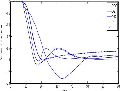
gradual increase in demand of 0.01 pu is applied to zone 1 The frequency deviation of the first area frequency and f1 and second f2 deviation of the area and the area between

clamping signal power closed loop system shown in Fig. 3,

4 and 5. Similarly a step increase in demand of 0.01 applies

to Area2.frequency deviation of the first area and the f1

and f2 frequency of the second area and the area between

clamping signal powercircuitry of theclosed loop system

[image:6.612.322.539.129.431.2]

are shown in Fig.6,7,8.

Table 1: Parameters of the controller to the system using

different controllers

Kp Ki Kd

PSO 1.34 3.48 1.2

DE 2.28 0.1514 0.8464

PID 0.933 0.7185 0.4198

PI 1.01 1.6974 -

I - 1.46 -

Simulation results show improved performance in the time domain specifications for a load of 0.01 pu step Using the PSO approach, global and local solutions could be found simultaneously for a better adjustment of the controller

parameters .The PID value that was obtained by the PSO

algorithm is compared with the PID controller derived from differential evolution algorithm, PID controller, PI controller and the I in different perspectives namely,

robustness and stability. All simulations were carried out

using MATLAB A comparison of time domain specifications overshoot and settling time for a load of 0.01 pu step in area 1 are tabulated as given in the table (2) and it is very clearly that the PSO based controller dramatically reduces

overshoot by a large value.Settling time improved.

Table 2: Analysis of the system performance by using

different methods of setting the controller

Settling Time Max.Overshoot

PSO 8.4 0.0098

DE 9.06 0.0103

PID 13.76 0.078

PI 8 0.07

I 9.94 0.09

0 10 20 30 40 50 60 70

-1.4 -1.2 -1 -0.8 -0.6 -0.4 -0.2 0

Time

Fr

eq

u

en

c

y

D

ev

ia

ti

o

n

PSO DE PID PI I

Fig.3.Change in frequency of the Zone-1 for 1% change in

the area-1

0 10 20 30 40 50 60 70

-1.4 -1.2 -1 -0.8 -0.6 -0.4 -0.2 0

time

f

r

eq

u

en

c

y

d

ev

ia

ti

o

n

PSO DE PID PI I

Fig.4.Change in frequency of the Zone-2 for 1% change in

[image:6.612.36.253.340.471.2] [image:6.612.327.519.476.622.2]

(7)

Page 869

0 10 20 30 40 50 60 70

-0.4 -0.3 -0.2 -0.1 0 0.1 0.2 0.3 time ti el in e p o w er d ev ia ti o n PSO DE PID PI I

Fig.5.Change in linking power lines to the 1% change in

the area-1

0 10 20 30 40 50 60 70

-1.4 -1.2 -1 -0.8 -0.6 -0.4 -0.2 0 time fr eq u en c y d ev ia io n PSO DE PID PI I

Fig.6. Change Frequency Zone-1 for the 1% change in the

area-2

0 10 20 30 40 50 60 70

-1.4 -1.2 -1 -0.8 -0.6 -0.4 -0.2 0 time fr eq u en c y d ev ia ti o n PSO DE PID PI I

Fig.7.Change in frequency of the Zone-2 for 1% change in

the area-2

0 10 20 30 40 50 60 70

-0.4 -0.3 -0.2 -0.1 0 0.1 0.2 0.3 time T iel in e p o w er d ev ia ti o n PSO DE PID PI I

Fig.8.Change in linking power lines to the 1% change in

the area-2

7. Conclusion

Load Frequency Control (LFC) system power supply multiple units with different sources of electricity generation and thermal, hydro and gas power plants is presented in this paper. The controller parameters are optimized using Swarm Optimization technique particles (PSO). Initially, Multi System Multi Area Power source is considered and the control parameters PSO technique is tuned by performing multiple runs of the algorithm for each variation of control parameters. The parameters Proportional Integral Derivative (PID) are optimized using PSO optimization technique. The superiority of the proposed approach has been demonstrated by comparing the results with integral controller (I), proportional integral controller (PI), Proportional Integral Derivative (PID) controller and the PID controller used for the same energy systems using various performance measures such as settling time and criteria of standard frequency error sedimentation and tie-line power deviation after a load disturbance step (SLP). It is noted that the dynamic performance of the proposed controller is improved. Furthermore, it is also noted that the proposed system is robust and not affected by the change in the load condition, the system parameters and the size of SLPs.

Appendix B: System Settings

(8)

Page 870

REFERENCES

[1] Banaja Mohanty, Sidhartha panda, PK Hota., Controller tuning parameters of differential evolution algorithm and its application to load frequency control system of multi-source energy, electric power and energy systems 54 (

2014) 77-85

[2] Kennedy, J., Eberhart, RC, Particle Swarm

Optimization,Proc.IEEE International

Conference on Neural Networks, Perth

Australia, IEEE Service Center, Piscataway, NJ,

IV: 1942-1948, 1995.

[3] gaing, ZL., A Particle Swarm Optimization

Approach for the optimal design of PID

In AVR system controller, IEEE Transactions

Energy conversion, Vol.19, No.2, June

2004.

[4] Kim Dong Hwa and Park Jin Ill Intelligent PID Controller Setting the AVR system using GA and PSO

Springer-Verlag Berlin Heidelberg :. ICIC 2005, Part II,

LNCS 3645, pp 366-375 (2005).

[5] stability and system control Kundur P. Power. New

York: Mc-Grall Hill;1994.

[6] Elgerd OI.Electricity systems theory introduces energy.

New Delhi: Tata

McGraw-Hill;1983.

[7] frequency control Hassan B. robust feed system. New

York: Springer;2.009.

[8] Ibraheem, Kumar P, DP Kothari. Recent philosophies

automatic generation

control strategies energy systems. IEEE Trans Power Syst

2005;20: 346-57.

[9] Parmar KPS, Majhi S, DP Kothari. Load frequency

control of real power

generation system with multi-source energy. Int J Syst

Energy Power Elect

2012;42: 426-33.

[10] DK Chaturvedi, Satsangi PS, PK Kalra. Control load

frequency: A general neural network approach.Electronic

Power Energy Syst 1999;21: 405-15.

[11] Ghosal SP.The optimization of the PID gains particle

swarm optimization fuzzy automatic generation control

based.Electr Power Syst Res 2004;72: 203-12.

[12] Ahamed TPI, PSN Rao, PS Sastry. A reinforcement

learning approach ofautomatic generation control. Electr

Power Syst Res 2002;63: 09/26.

[13] Khuntia SR, Panda S. simulation study for the automatic control of generating a

multi-power system ANFIS focus area. Soft Comput Appl 2012; 12: 333-41.

[14] Saikia LC, J Nanda, S. Mishra Performance comparison of several classical

AGC controllers for multiple interconnected areas thermal system. Int J Elect

Energy Power Syst 2011; 33: 394-401.

[15] Nanda J, Mishra S, Saikia LC. Maiden application based bacterial foraging

optimization technique in controlling automatic

generation multiarea. IEEE Trans Power Syst 2009; 24: 602-9.

BIOGRAPHIES

V.Jyothi currently pursuing M.Tech in Control Systems at JNTUA College of Engineering and Technology Anantapur, Andhra Pradesh. Her area of interest is Control Systems.