New estimations on the upper bounds for the nuclear norm of a tensor

R E S E A R C H

Open Access

New estimations on the upper bounds for

the nuclear norm of a tensor

Xu Kong

_{, Jicheng Li}

_{and Xiaolong Wang}

*_{Correspondence:} [email protected]

1_{School of Mathematical Sciences,} Liaocheng University, Liaocheng, China

Full list of author information is available at the end of the article

Abstract

Using the orthogonal rank of the tensor, a new estimation method for the upper bounds on the nuclear norms is presented and some new tight upper bounds on the nuclear norms are established. Taking into account the structure information of the tensor, an important factor affecting the upper bounds is discussed and some corresponding properties related to the nuclear norms are given. Meanwhile, some new results of the upper bounds on the nuclear norms are obtained.

MSC: 15A18; 15A69

Keywords: Tensor; Nuclear norm; Orthogonal rank; Upper bound

1 Introduction

A tensor is a multidimensional array that can provide a natural and convenient way for representing the multidimensional data such as discrete forms of multivariate functions, images, video sequences, and so on [1,2,10,14]. With the successful and widespread use of the matrix nuclear norm (a sum of the singular values) in the information recovery, the research on the nuclear norm of the tensor (see Definition2.3in Sect.2) has been a hot topic in both the theory and applications [5–8].

A natural problem is how to compute the nuclear norm of a tensor. Unfortunately, com-pared with the matrix nuclear norm, the nuclear norm of a tensor is closely related to the number field, and the computation of the tensor nuclear norm is NP-hard [5]. Thus, ex-ploring some simple polynomial-time computable upper bounds on the nuclear norm is very important.

Relating to the nuclear norm of a tensor, Friedland and Lim established the following upper bound through the Frobenius norm of this tensor in [5].

Theorem 1.1([5]) LetX∈Rn1×···×nD_.Then

X∗≤

D

i=1

niXF.

In [8], Hu established a tighter upper bound.

Theorem 1.2(Lemma 5.1 in [8]) LetX∈Rn1×···×nD_.Then

X∗≤

D i=1ni

max{n1, . . . ,nD}

XF. (1)

Furthermore, Hu established another upper bound on the nuclear norm of a tensor through the nuclear norms of its unfolding matrices.

Theorem 1.3(Theorem 5.2 in [8]) LetX∈Rn1×···×nD_.Then

X∗≤

D i=2ni

max{n2, . . . ,nD}

X(1)∗. (2)

In this paper, we present some new upper bounds on the nuclear norms through using the orthogonal rank of the tensor [9,12]. Furthermore, taking into account the structure information of the tensor, some new results of the upper bounds on the nuclear norms are obtained.

Since the spectral norm and nuclear norm of a tensor are closely related to the num-ber field [6], for the sake of simplicity, we always assume that the tensors discussed are nonzero real tensors, and unless mentioned otherwise, we just discuss the spectral and the nuclear norm over the real field. Some corresponding notations are as follows: a ten-sor is denoted by the calligraphic letter (e.g.,X), while the scalar is denoted by the plain letter, and matrices and vectors are denoted by bold letters (e.g., X and x).

The rest of the paper is organized as follows. In Sect.2, we recall some definitions and related results which are needed for the subsequent sections. In Sect.3, we present the upper bounds on the nuclear norms of general tensors and discuss the factor affecting the upper bounds. Finally, some conclusions are made in Sect.4.

2 Notations and preliminaries

This section is devoted to reviewing some conceptions and results related to tensors, which are needed for the following sections.

Firstly, we discuss the unfolding matrix or matrix representation of a tensor. Let X = (xi1···iD)∈R

n1×···×nD_{. Then, by organizing several indexes of} X _{and the} re-maining indexes of X as the row index and the column index, respectively, the ten-sor X can be reshaped into a matrix form [13]. Especially, if the number of row in-dex is equal to one, then we get the mode-d matricization X(d), the columns of which are the mode-d fibers of the tensor (obtained by fixing every coordinate except one, [xi1···id–11id+1···iD, . . . ,xi1···id–1ndid+1···iD]

T_{), arranged in a cyclic ordering; see [3] for details.}

Contrary to the operation above, a matrix can also be reshaped into a tensor by using the opposite operation.

In what follows, we review some definitions of the tensor norms.

Definition 2.1 ([3]) Let X = (xi1···iD)∈ R

n1×···×nD_{, the Frobenius norm or Hilbert–} Schmidt norm of the tensorXis defined as

XF=

X,X=

n1

i1=1

· · ·

nD

iD=1 x2_i1···iD

Definition 2.2([6]) Let “◦” denote the outer product operation. The spectral norm of X∈Rn1×···×nD _{is defined as}

X2=max

X, x(1)◦ · · · ◦x(D): x(d)∈Rnd_,x(d)

2= 1, 1≤d≤D

.

Furthermore,X2is equal to the Frobenius norm of the best rank-one approximation of the tensorX.

Similar to the matrix case, the nuclear norm can be defined through the dual norm of the spectral norm.

Definition 2.3([6]) LetX∈Rn1×···×nD_{, the nuclear norm of}X_{is defined as the dual norm} of the spectral norm. That is,

X∗:=maxX,Y:Y∈Rn1×···×nD_,Y 2= 1

. (3)

For the nuclear norm defined by (3), it can be shown that

X∗=min

_P

p=1

|λp|:X= P

p=1

λpx(1)p ◦ · · · ◦x(pD),

x(d)

p 2= 1, x (d)

p ∈Rnd,λp∈R,P∈N

.

Another important concept related to the matrix and the tensor is the mode-d multipli-cation.

Definition 2.4([3]) LetX = (xi1···iD)∈Rn1×···×nD. Then the mode-dmultiplication ofX by the matrix U = (uij)∈Rnd×ndis defined by

(X×dU)i1···id–1idid+1···iD=

nd

id=1

xi1···id–1idid+1···iDui_did, 1≤d≤D.

It should be mentioned that the mode-dmultiplication is also available forn_d= 1. Furthermore, let

W(1), . . . , W(D)·X=X×1W(1)× · · · ×DW(D).

If for all 1≤d≤Dthe matrices W(d)_{are orthogonal matrices (W}(d)_W(d)T

is an identity matrix), then (W(1)_{, . . . , W}(D)_{)·Xis called a multi-linear orthogonal transformation of the} tensorX.

Finally in this section, we introduce the tool used in the paper for the estimation of the upper bounds.

Definition 2.5([9]) The orthogonal rank ofX∈Rn1×···nD_{is defined as the smallest} num-berRsuch that

X=

R

r=1

whereUr(1≤r≤R) are rank-one tensors such thatUr1,Ur2= 0, (r1=r2) for 1≤r1≤R and 1≤r2≤R.

The decomposition ofX given by (4) is also called the orthogonal decomposition of the tensorX.

For the orthogonal rank of a tensor, the following conclusion is true.

Theorem 2.1([11]) Let n1≤ · · · ≤nD.Then,for anyX∈Rn1×···×nD,it holds

r⊥(X)≤

D–1

i=1 ni,

where r⊥(X)denotes the orthogonal rank ofX.

Noting the fact that indices relabeling does not change the tensor orthogonal rank, then by Theorem2.1, we have that, for anyX∈Rn1×···×nD_{, it holds}

r⊥(X)≤

D

i=1ni

max{n1, . . . ,nD}

. (5)

Especially, for the third order tensor, the following result was established in [11].

Lemma 2.1([11]) Let n≥2.Then,for anyX∈Rn×n×2_{,the following holds:}

r⊥(X)≤

2n– 1, if n is odd; 2n, if n is even.

3 Upper bounds of the nuclear norm

In this section, we discuss the upper bounds on the nuclear norm of a tensor. Meanwhile, some properties and polynomial-time computable bounds related to the nuclear norm will be given.

3.1 Upper bounds given by the Frobenius norm

In this subsection, we use the orthogonal rank of a general tensor to establish the upper bounds on the nuclear norm through the Frobenius norm of this tensor.

Theorem 3.1 LetX∈Rn1×···×nD_{.Suppose that} R= max

Y∈Rn₁×···×nD

rank_⊥(Y).

Then

X∗≤√RXF. (6)

Proof LetY∈Rn1×···×nD_{be an arbitrary nonzero tensor and the orthogonal rank of}Y_be Ry. Suppose that

Y=

Ry

r=1 Ur

Then, according to the properties of the orthogonal rank decomposition and the best rank-one approximation, we have

Y2≥ max 1≤r≤Ry

UrF

(7)

and

Y2

F= Ry

r=1

Ur2F. (8)

Without loss of generality, suppose that

U1F= max

1≤r≤Ry

UrF

.

Then it follows from (7) and (8) that

X, Y

Y2

≤ XF

YF

Y2

≤ XF

Ry

r=1Ur2F

U1F

≤ XF

RyU12F

U1F

=RyXF

≤√RXF. (9)

Thus, according to the arbitrariness ofYand (9), we get

max

Y∈Rn₁×···×nD

X, Y

Y2

≤√RXF.

Noting the definition of the nuclear norm (Definition2.3), the conclusion is established.

Remark3.1 Comparing the upper bound given by (6) with the upper bound given by (1), which is obtained in [8], the new upper bound given by (6) is tighter.

Actually, it follows from (5) that the upper bound given by (6) improves the upper bound given by (1).

More specifically, we present a simple example to show that the upper bound given by Theorem3.1not only can be tighter than the upper bound given by (1) but also a sharp bound.

Example3.1 Let

A=

⎡ ⎢ ⎣

0 1 0 1 0 0 0 0 0

–1 0 0

0 1 0

0 0 1

⎤ ⎥

By Theorem3.1and Lemma2.1, we get

A∗≤√512_{+ 1}2_{+ (–1)}2_{+ 1}2_{+ 1}2_{= 5 <}

"

3×3×2 3

√

5 =√30.

This means that the upper bound given by (3.1) is tighter than the upper bound given by (1).

Furthermore, by a simple computation, we getA2= 1. Then it follows from the defi-nition of the nuclear norm that

A∗≥

A,_AA 2

=A 2

F

A2 =5

1= 5.

Thus, it holds

A∗= 5.

Actually,

A= e1;3◦e2;3◦e1;2+ e2;3◦e1;3◦e1;2+ (–e1;3)◦e1;3◦e2;2+ e2;3◦e2;3◦e2;2

+ e3;3◦e3;3◦e2;2 (10)

is a nuclear decomposition ofA, where e1;3= [1, 0, 0]T, e2;3= [0, 1, 0]T, e3;3= [0, 0, 1]T,

e1;2= [1, 0]T, and e2;2= [0, 1]T. Since

A, e1;3◦e2;3◦e1;2=A, e2;3◦e1;3◦e1;2=

A, (–e1;3)◦e1;3◦e2;2

=A, e2;3◦e2;3◦e2;2=A, e3;3◦e3;3◦e2;2,

then, according to the sufficient and necessary conditions of the nuclear norm decompo-sition obtained in [6], we get that (10) is a nuclear decomposition ofA.

This also means that the upper bound given by Theorem3.1is a sharp upper bound of the nuclear norm.

3.2 Upper bounds given by nuclear norms of the unfolding matrices of a tensor

In this subsection, we present a new way to establish the upper bounds on the nuclear norm of a tensor through the nuclear norms of the unfolding matrices of this tensor.

Theorem 3.2 LetX∈Rn1×···×nD_{.Suppose that}

˜

R= max

Y∈Rn2×···×nD

rank⊥(Y).

Then

X∗≤R˜X(1)∗. (11)

Proof Let the singular value decomposition of the matrix X(1)be

X(1)=σ1u1vT1 +· · ·+σSuSvTS, (12)

Then equality (12) can be expressed as the following form:

X=σ1u1◦V1+· · ·+σSuS◦VS, (13)

whereVs∈Rn2×···×nDare obtained by reordering the vector vsinto (D– 1)th order tensor

with a certain order, 1≤s≤S. Suppose that the orthogonal rank decomposition ofVsis

Vs= v(1,1 s)◦ · · · ◦v (D–1,s)

1 +· · ·+ v (1,s)

Ps ◦ · · · ◦v (D–1,s)

Ps , 1≤s≤S.

Then, by taking the expression ofVsinto the right-hand side of (13), we get

X=σ1

P1

i=1

u1◦v(1,1)i ◦ · · · ◦v

(D–1,1)

i +· · ·+σS PS

i=1

u1◦v(1,i S)◦ · · · ◦v

(D–1,S)

i

=σ1

P1

i=1

v(1,1)_{i 2}· · ·v_i(D–1,1)₂u1◦

v(1,1)_i

v(1,1)_i 2

◦ · · · ◦ v

(D–1,1)

i

v(_iD–1,1)2 +· · ·

+σS PS

i=1

v(1,s)

i 2· · ·v (D–1,s)

i 2

u1◦

v_i(1,S)

v_i(1,S)₂ ◦ · · · ◦

v(_iD–1,S)

v_i(D–1,S)₂. (14)

Noting that

Vs2F= Ps

i=1

v(1,s)

i ◦ · · · ◦v

(D–1,s)

i 2 F= Ps i=1

v(1,s)

i

2

F· · ·v

(D–1,s)

i

2

F=vs

2

F= 1, (15)

wherePs≤ ˜R, 1≤s≤S, then it follows from the definition of the nuclear norm and (14)

that

X∗≤σ1

P1

i=1

v(1,1)_{i 2}· · ·v_i(D–1,1)₂+· · ·+σS PS

i=1

v_i(1,s)₂· · ·v(_iD–1,s)₂

≤σ1

P1+· · ·+σS

PS

by (15) and Cauchy-Schwarz inequality

≤σ1

˜

R+· · ·+σS

˜ R = ˜

RX(1)∗.

Remark3.2 Comparing the upper bound given by (11) with the upper bound given by (2), which is obtained in [8], the new upper bound given by (11) is smaller.

Actually, it follows from inequality (5) that the upper bound given by (11) improves the upper bound given by (2).

Similar to the discussion of Hu [8], the upper bounds can also be obtained by other unfolding ways and further improved by considering the multi-linear ranks of a tensor (ranks of the unfolding matrices).

Corollary 3.1 LetX∈Rn1×n2×n3 _{and r}

d=rank(X(d)), 1≤d≤3.Then

X∗≤ √

min{r2,r3}X(1)∗+

√

min{r3,r1}X(2)∗+

√

min{r1,r2}X(3)∗

Proof According to the conditions of the corollary and the higher order singular value decomposition of the tensor [3], the tensorX can be expressed as

X=W(1), W(2), W(3)· ˜X,

whereX˜∈Rr1×r2×r3_{and W}(d)∈Rnd×rd_{satisfying that W}(d)T_W(d)_{is an identity matrix for} all 1≤d≤3.

By the definition of the tensor nuclear norm (Definition2.3), one can easily verify the following conclusions:

˜X∗=X∗, (16)

and

˜X(1)∗=X(1)∗. (17)

It follows from Theorem3.2and (17) that

˜X∗≤" max

Y∈Rr₂×r₃

rank_⊥(Y) ˜X(1)∗≤

min{r2,r3}X(1)∗.

Noting (16), we get

X∗≤min{r2,r3}X(1)∗.

Similarly, we have

X∗≤min{r3,r1}X(2)∗,

and

X∗≤min{r1,r2}X(3)∗.

Thus, the conclusion is obtained.

3.3 Factors affecting the upper bounds on the nuclear norm and further results

In this subsection, we discuss the factors affecting the nuclear norm of a tensor. Especially, we focus on the structure analysis of a tensor. Based on the discussion, some new upper bounds on the nuclear norms of tensors are presented.

Firstly, we give a simple example to illustrate that the nuclear norm of a tensor is closely related to the structure of this tensor.

Example3.2 Let

A=

#

0 1 1 0

–1 0 0 1

$

Similar to the discussion of Example3.1, since

A= e1;2◦e2;2◦e1;2+ e2;2◦e1;2◦e1;2+ (–e1;2)◦e1;2◦e2;2+ e2;2◦e2;2◦e2;2

and

A, e1;2◦e2;2◦e1;2=A, e2;2◦e1;2◦e1;2=

A, (–e1;2)◦e1;2◦e2;2

=A, e2;2◦e2;2◦e2;2,

then, according to the sufficient and necessary conditions of the nuclear norm decompo-sition obtained in [6], we get

A∗= 4.

It is well known that the nuclear norm of a tensor is closely related to the number field [6]. Actually, the tensorAcan be expressed as the following form:

A=1 2

#

–1 –i

$

◦

#

1 i

$

◦

#

i 1

$

+1 2

#

–1 i

$

◦

#

1 –i

$

◦

#

–i 1

$

.

Let

W(1)=√1 2

#

–1 i –1 –i

$

, W(2)=√1 2

#

1 –i 1 i

$

, W(3)=√1 2

#

–i 1 i 1

$

.

Then it holds

W(1), W(2), W(3)·A=

#_√

2 0

0 0

0 0

0 √2

$

. (19)

For the sake of convenience, letAˆ= (W(1), W(2), W(3))·A. Then, using the same method as above, we have

ˆA, e1;2◦e1;2◦e1;2= ˆA, e2;2◦e2;2◦e2;2.

Thus ˆA∗= 2√2. Since all three matrices W(k)_{(1≤k≤3) are unitary matrices, based} on the invariance of the Frobenius norm of a tensor under the multi-linear orthogonal transformations, we get

A∗= ˆA∗= 2√2.

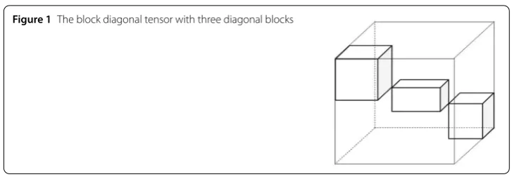
Figure 1The block diagonal tensor with three diagonal blocks

LetA= (ai1···iD)∈Rn1×···×nD andB= (bj1···jD)∈Rn1×···×nD, then the direct sum ofAand Bis an order-DtensorC= (ci1···iD) =A⊕B∈R

(n1+n₁)×···×(nD+nD)_{defined by}

ci1···iD=

⎧ ⎪ ⎪ ⎨ ⎪ ⎪ ⎩

ai1···iD, if 1≤iα≤nα,α= 1, 2, . . . ,D;

bi1–n1,...,iD–nD, ifnα+ 1≤iα≤nα+nα,α= 1, 2, . . . ,D;

0, otherwise.

Based on the discussion above, we present some properties of the spectral norm and nuclear norm of the tensor.

Lemma 3.1 LetX(l)_∈Rn(1l)×···×n (l)

D, 1≤l≤L,and

X=X(1)⊕ · · · ⊕X(L)∈R(

L l=1n

(l) 1)×···×(

L l=1n

(l) D)_.

Then

X2=max 1≤l≤L

_X(l) 2

. (20)

Proof According to the definition of the spectral norm of a tensor (Definition2.3), it is easy to get

X2≥max 1≤l≤L

_X(l) 2

.

Thus, the rest of the proof just needs to show

X2≤max 1≤l≤L

_X(l) 2

. (21)

Firstly, we consider the case of the third order tensors. Suppose thatX(l)_∈Rn(₁l)×n₂(l)×n(₃l)_(1≤l≤L),

X=X(1)⊕ · · · ⊕X(L)∈R(Ll=1n (l) 1)×(

L l=1n

(l) 2)×(

L l=1n

(l) 3 )_,

andσu◦v◦wis the best rank-one approximation ofX, whereσ=X2, u∈R

L l=1n

(l) 1 , v∈ RL

l=1n (l)

2 _{, w = [w}T

1, . . . , wLT]T∈R

L l=1n

(l)

3 _{, wl}∈Rn (l)

Then the following matrix

X×3wT=

⎡ ⎢ ⎢ ⎣

X(1)_× 3wT1

. ..

X(L)_× 3wLT

⎤ ⎥ ⎥ ⎦

is a block diagonal matrix. It follows

X2=X×3wT₂=max 1≤l≤L

_X(l)_× 3wTl2

≤max

1≤l≤L

_X(l) 2

.

Hence, inequality (21) is proved. This also implies that equality (20) is true for the third order tensors.

Secondly, for the case of higher order tensors with order larger than or equal to four, the same result can be established by the recursive method.

In all, the conclusion is true.

Then, based on Lemma3.1, the following two results related to the nuclear norms of tensors can be established.

Lemma 3.2 LetO∈Rn(1)1 ×···×n (1)

D _{be a zero tensor,and}X∈Rn (2) 1 ×···×n

(2) D _.Then

O⊕X∗=X⊕O∗=X∗.

Proof Suppose that

X∗=

P

p=1

|σp|

and

X=

P

p=1

σpx(1)p ◦ · · · ◦x(pD),

where for all 1≤p≤P, x(1)p ◦ · · · ◦x(pD)are rank-one tensors withx(1)p 2=· · ·=x(pD)2= 1. Then

O⊕X=

P

p=1

σp

x(1)p

0

◦ · · · ◦ x

(D)

p

0

,

where all 0sdenote zero vectors with suitable dimensions. This implies

O⊕X∗≤ X∗.

Furthermore, assume that

X∗=X,Y,

whereY∈Rn(2)1 ×···×n (2)

Then, by Lemma3.1, we have

O⊕Y2=Y2= 1.

It follows from Definition2.5that

O⊕X∗≥ O⊕X,O⊕Y=X,Y=X∗.

Thus it holdsO⊕X∗=X∗.

Using the same method, the equalityX⊕O∗=X∗can be proved.

Lemma 3.3 LetX(l)∈Rn(1l)×···×n (l)

D_{, 1}≤_l≤_L,and

X=X(1)⊕ · · · ⊕X(L)∈R(Ll=1n (l) 1)×···×(

L l=1n

(l) D)_.

Then

X∗=

L

l=1

_X(l)

∗.

Proof We just need to prove the case ofL= 2. For the general case, the conclusion can be obtained in a recursive way.

Let

˜

X1=X(1)⊕O(1), X˜2=O(2)⊕X(1),

whereO(1)_∈Rn(2)₁ ×···×n(2)_{D andO}(2)_∈Rn(1)₁ ×···×n(1)_{D are both zero tensors.}

Then, by using Lemma3.2, we get

X∗= ˜X1+X˜2∗≤ ˜X1∗+ ˜X2∗=X(1)_∗+X(2)_∗. (22)

Suppose that

_X(l)

∗=

X(l)_,Y(l)_{, and Y}(l)_∈Rn(1l)×···×n (l) D_,Y(l)

2= 1.

Then, by Lemma3.1, we get

_Y(1)_⊕Y(2) 2= 1.

Thus, according to Definition2.5, we have

X∗= max

Y∈R(n(1)_{1 +}n(2)_{1 )}×···×(n(1) D+n

(2) D)

Y2=1

X,Y

≥X(1)_⊕X(2)_,Y(1)_⊕Y(2)

=X(1)_∗+X(2)_∗. (23)

Based on the fact that the nuclear norm of a tensor is also kept invariant under the multi-linear orthogonal transformation, we get the following result.

Corollary 3.2 LetX∈Rn1×···×nD_{.If the tensor}X _{admits a diagonal structure under the} multi-linear orthogonal transformations,then

X∗=

P

p=1

|σp|,

whereσp(1≤p≤P)are the diagonal elements and P≤n1.

This case presented by Corollary3.2is consistent with the definition of the nuclear norm of the matrix case, and in this case, the nuclear norm of the tensor can be accurately cal-culated.

Taking into account the structure information of the tensor, some new results of the upper bounds on the nuclear norms can be obtained. For the convenience of comparison, we just present the upper bounds on the nuclear norms of tensors through the dimensions of the tensors, without considering the orthogonal rank of the tensors.

Theorem 3.3 LetX∈Rn1×···×nD _{and L be the maximum number of diagonal blocks that} the tensorX can attain under the multi-linear orthogonal transformations.Suppose that the size of each diagonal block is n(₁l)× · · · ×n(_Dl)and

˜

nl=

D

i=1n (l)

i

max{n(₁l)· · ·n_D(l)}, 1≤l≤L. Then it holds

X∗≤

L

l=1

˜

nlXF. (24)

Proof Assume that

X=D(X)×1W(1)· · · ×DW(D),

where

D(X) =D(1)⊕ · · · ⊕D(L)

and W(d)∈Rnd×nd₍₁≤_d≤_{D) are orthogonal matrices,}D(l)∈Rn(1l)×···×n (l)

D_{, 1}≤_l≤_L. Then it follows from the invariance of the Frobenius norm of a tensor under the multi-linear orthogonal transformation that

X2

F= L

l=1

_D(l)2

Furthermore, since the nuclear norm of a tensor is also kept invariant under the multi-linear orthogonal transformation, we get

X∗=D(X)_∗.

Hence, by Lemma3.3and (25), we get

X∗=D(X)_∗

=

L

l=1

_D(l)

∗

≤

L

l=1

˜

nlD(l)_F

≤

L

l=1

˜

nl

L

l=1

_D(l)2

F (by Cauchy-Schwarz inequality)

=

L

l=1

˜

nlXF.

Without loss of generality, suppose that

nD=max{n1, . . . ,nD}.

Since

n1=

L

l=1 n(₁l) ..

.

nD–1=

L

l=1 n(_Dl)_–1,

it is easy to get

D

i=1ni

max{n1, . . . ,nD}

=

D–1

i=1 ni

=

L

l=1 n(1l)

· · ·

L

l=1 n(_Dl)_–1

≥

L

l=1

˜

nl.

Thus, the upper bound given by (24) improves (1). Theorem3.3also shows that the upper bound on the nuclear norm can be improved by using the structural information.

Theorem 3.4 LetX∈Rn1×···×nD_{,and L be the maximum number of diagonal blocks that} the tensorX can attain under the multi-linear orthogonal transformations.Suppose that the size of each diagonal block is n(₁l)× · · · ×n(_Dl),and

˜

nl=

D

i=2n (l)

i

max{n(₂l)· · ·n_D(l)}, 1≤l≤L, and

˜

n=max

1≤l≤L{˜nl}.

Then it holds

X∗≤√n˜X(1)∗. (26)

Proof Similar to the proof of Theorem3.3, assume

X=D(X)×1W(1)· · · ×DW(D),

where

D(X) =D(1)⊕ · · · ⊕D(L)

and W(d)_∈Rnd×nd₍₁≤_d≤_{D) are orthogonal matrices.} Then it holds

X∗=D(X)_∗

=

L

l=1

_D(l)

∗

≤

L

l=1

˜

nlD((1)l)∗

≤√n˜

L

l=1

D(l) (1)∗

≤√n˜

L

l=1

D(1)∗

=√n˜X(1)∗.

Example3.3 LetAbe defined in Example3.2, and

B=A⊕A

=

⎡ ⎢ ⎢ ⎢ ⎣

0 1 0 0 1 0 0 0 0 0 0 0 0 0 0 0

–1 0 0 0

0 1 0 0

0 0 0 0

0 0 0 0

0 0 0 0 0 0 0 0 0 0 0 1 0 0 1 0

0 0 0 0

0 0 0 0

0 0 –1 0

0 0 0 1

⎤ ⎥ ⎥ ⎥ ⎦.

Then, by Theorem1.2, we get

B∗≤√4∗4BF= 8

√

2.

It follows from Theorem3.4that

B∗≤√2∗2BF= 4

√

2.

There has been a marked improvement in the upper bounds on the nuclear norm.

4 Conclusions

In this paper, we provide a new estimation method for the upper bounds on the nuclear norms and obtain some new upper bounds related to the nuclear norms. Meanwhile, it is found that the upper bounds on the nuclear norms are not only related to the dimensions of the tensor but also to the structure of the tensor. Taking into consideration the structure information of the tensor, the upper bounds on the nuclear norms can be improved.

Funding

This research work was supported by the Natural Science Foundation of China (NSFC) (Nos: 11401286, 11671318, 11401472), Natural Science Foundation of Shaanxi Province (No: 2014JM1029), and Scientific Research Foundation of Liaocheng University.

Competing interests

All three authors declare that they have no competing interests.

Authors’ contributions

All three authors contributed equally to this work. All authors read and approved the final manuscript.

Author details

1_{School of Mathematical Sciences, Liaocheng University, Liaocheng, China.}2_{School of Mathematics and Statistics, Xi’an}

Jiaotong University, Xi’an, China.3_{School of Science, Northwestern Polytechnical University, Xi’an, China.}

Publisher’s Note

Springer Nature remains neutral with regard to jurisdictional claims in published maps and institutional affiliations.

Received: 11 July 2018 Accepted: 20 September 2018

References

1. Che, M.L., Cichocki, A., Wei, Y.M.: Neural networks for computing best rank-one approximations of tensors and its applications. Neurocomputing267, 114–133 (2017)

2. Cichocki, A., Mandicand, D., Pan, A.-H., Caiafa, C., Zhou, G., Zhao, Q., De Lathauwer, L.: Tensor decompositions for signal processing applications: from two-way to multiway component analysis. IEEE Signal Process. Mag.32(2), 145–163 (2015)

3. De Lathauwer, L., De Moor, B., Vandewalle, J.: A multilinear singular value decomposition. SIAM J. Matrix Anal. Appl. 21(4), 1253–1278 (2000)

4. De Silva, V., Lim, L.H.: Tensor rank and the ill-posedness of the best low-rank approximation problem. SIAM J. Matrix Anal. Appl.30(3), 1084–1127 (2008)

6. Friedland, S., Lim, L.H.: Nuclear norm of higher-order tensors. Math. Comput.87(311), 1255–1281 (2018) 7. Gandy, S., Recht, B., Yamada, I.: Tensor completion and low-n-rank tensor recovery via convex optimization. Inverse

Probl.27(2), 025010 (2011)

8. Hu, S.L.: Relations of the nuclear norm of a tensor and its matrix flattenings. Linear Algebra Appl.478, 188–199 (2015) 9. Kolda, T.G., Bader, B.W.: Orthogonal tensor decomposition. SIAM J. Matrix Anal. Appl.23, 243–255 (2001)

10. Kolda, T.G., Bader, B.W.: Tensor decompositions and applications. SIAM Rev.51(3), 455–500 (2009)

11. Kong, X., Meng, D.Y.: The bounds for the best rank-1 approximation ratio of a finite dimensional tensor space. Pac. J. Optim.11, 323–337 (2015)

12. Li, Z., Nakatsukasa, Y., Soma, T., Uschmajew, A.: On orthogonal tensors and best rank-one approximation ratio. SIAM J. Matrix Anal. Appl.39(1), 400–425 (2018)

13. Oseledets, I.V., Tyrtyshnikov, E.E.: Breaking the curse of dimensionality, or how to use SVD in many dimensions. SIAM J. Sci. Comput.31(5), 3744–3759 (2009)