Estimation in a Cox Proportional Hazards Cure Model

BIOMETRICS 56, 227-236 March 2000

Estimation in a

Cox

Proportional Hazards Cure Model

Judy P. Sy

Biostatistics, Genentech

Inc., 1

DNA Way, South S a n Francisco, California

94080, U.S.A.

and

Jeremy

M. G.

Taylor

Department of Biostatistics, University of Michigan, A n n Arbor, Michigan

48109,

U.S.A.

email:

j

mgt

@umich .edu

SUMMARY. Some failure time data come from a population that consists of some subjects who are suscep- tible to and others who are nonsusceptible to the event of interest. The data typically have heavy censoring at the end of the follow-up period, and a standard survival analysis would not always be appropriate. In such situations where there is good scientific or empirical evidence of a nonsusceptible population, the mixture or cure model can be used (Farewell, 1982, Biometrics 38, 1041-1046). It assumes a binary distribution to model the incidence probability and a parametric failure time distribution to model the latency. Kuk and Chen (1992, Biometrika 79, 531-541) extended the model by using Cox’s proportional hazards regression for the latency. We develop maximum likelihood techniques for the joint estimation of the incidence and latency regression parameters in this model using the nonparametric form of the likelihood and an EM algorithm. A zero-tail constraint is used t o reduce the near nonidentifiability of the problem. The inverse of the observed information matrix is used t o compute the standard errors. A simulation study shows that the methods are competitive t o the parametric methods under ideal conditions and are generally better when censoring from loss to follow-up is heavy. The methods are applied to a data set of tonsil cancer patients treated with radiation therapy.

KEY WORDS: Cure model; EM algorithm; Product-limit estimate; Profile likelihood.

1. Introduction

In survival analysis, it is usually assumed that if complete follow-up were possible for all individuals, each would even- tually experience the event of interest. Sometimes’ however, the data come from a population where a substantial propor- tion of the individuals do not experience the event at the end of the observation period. In some situations, some of these survivors are actually cured in the sense that, even after an extended follow-up, no further events are observed. An ex- ample is patients with tonsil cancer treated using radiation therapy (Withers et al., 1995), in which cure occurs if the ra- diation kills all the cancer cells. For such data, Kaplan-Meier (K-M) estimates of the survival function for time t o local re- currence level off to nonzero proportions. Furthermore, there is a time window within which most or all of the recurrences are expected to occur, and so a patient without any recurrence beyond this window can usually be considered as being cured. This type of data is typical of diseases where the biology of the disease suggests the possibility of cure. A K-M survival curve that shows a long and stable plateau with heavy cen- soring at the tail may be taken as empirical evidence of a cured fraction. The use of standard survival analysis for such data may be inappropriate since not all the individuals are susceptible.

In a cure model, the population is a mixture of suscepti- ble and nonsusceptible (cured) individuals. The objective is usually to study the cure rate and survival distribution and the effect of any covariates. We are interested in whether the event can occur, which we call incidence, and when it will occur, given that it can occur, which we call latency. In the tonsil cancer application, there are two types of covariates, patient variables such as tumor stage and treatment variables such as total dose of irradiation. How these covariates influ- ence the cure rate would be viewed as most important, but there is also interest in how they relate t o when the recurrence happens.

Various parametric and nonparametric methods have been proposed for the cure model. Farewell (1982) used logistic regression for the mixture proportion and a Weibull regression model for the latency. Peng, Dear, and Denham (1998) used a generalized F for the latency distribution. Kuk and Chen (1992) proposed a semiparametric generalization of Farewell’s model using a Cox proportional hazards (PH) model in the susceptible group; we call this the PH cure model. They used an estimation method involving Monte Carlo simulation. In this paper, we present a different estimation method.

idence of a nonsusceptible population. The model generally requires long-term follow-up and large samples, and censor- ing from loss to follow-up during the period when events can occur must not be excessive. Otherwise, identifiability prob- lems between the incidence and latency parameters can occur. 2. The Proportional Hazards Cure Model

Let Y be the indicator that an individual will eventually (Y =

1) or never (Y = 0) experience the event, w i t h p = Pr(Y = 1). Let T denote the time to occurrence of the event, defined only when Y = 1, with density f ( t

I

Y = 1) and survival function

S ( t

I

Y = 1). For a censored individual, Y is not observed. The

marginal survival function of T is S ( t ) = (1 - p ) + p S ( t

I

Y =

1) for

t

<

m. Note that S ( t ) + 1 - p as

t

-+ 00. We assume

an independent, noninformative, random censoring model and that censoring is statistically independent of Y.

Farewell (1982) used a logistic regression model for the in- cidence p ( z ) = pr(Y = 1 ; x ) = exp(z’b)/(l +exp(z’b)), where the covariate vector z includes the intercept, and a parametric survival model for S ( t

I

Y = 1). Kuk and Chen (1992) general- ized this by using a Cox PH model with hazard function X ( t

I

Y = 1; z ) =

X o ( t I

Y = 1) exp(z’p), where z is a vector of co- variates other than the intercept and X o ( t

I

Y = 1) is the con- ditional baseline hazard function. Through b and P, the model is able to separate the covariates’ effects on the incidence and the latency and, in that sense, provide a flexible class of mod- els when there is a priori belief in a nonsusceptible group. For the Kuk and Chen model, the conditional cumulative hazard function is A(t

I

Y = 1; z ) = Ao(t

I

Y = 1) exp(z’P), where

Ao(t

I

Y = 1; z ) =

J;

Xo(u

I

Y = 1)du. The conditional sur-

vival function is

s(t

I

Y = 1; z ) =

so(t

I

Y =

where So(t

I

Y = 1) is the conditional baseline survival func- tion.

It is not difficult to see that a mixture of P H functions is no longer proportional and in fact, for a binary covariate, a PH cure model can have marginal survival curves that cross. However, the standard P H model is a special case of a PH cure model in which p ( z ) = 1 for all z.

The PH cure model is a special case of a multiplicative frailty model, in which the hazard for an individual, condi- tional on Y, can be written as X ( t

I

Y ;

z )

= YX(t

I

Y = 1; z ) .

As a frailty variable, Y is not entirely unobservable since an individual becomes labeled as Y = 1 if an event is observed. 3. Estimation

3.1 Maximum

Likelihood

Estimation

Denote the observed data for individual i by (ti, 6,, z i ) , i =

1,

.

. .

,

n, where ti is the observed event or censoring time, 6i =

1 if

ti

is uncensored and

Si

= 0 otherwise, and

zi

is a vector of covariates. For convenience, we let xi = (1, z i ) ’ , although the covariates in zi and zi do not have t o be identical. Denote the k distinct event times by

t ( l )

<

. . .

<

t ( k ) .

It follows that, if 6i = 1, yi = 1 and, if 6i = 0, yi is unobserved, where yi is the value taken by the random variable Yi. The likelihood contribution of individual i is p , f ( t i

I

Y = l ; z a )

for 6i =

1

and (1 - p i )

+

piS(ti

I

Y = 1; zi) for 6i = 0, where pi = pr(Y, = 1; zi). For the P H cure model, the observed full likelihood is then

L(b,

P,

We want to obtain the estimates

6

and

B

that maximize

L(b,P,Ao). In the ordinary Cox PH model, the standard

analysis is to use the partial likelihood that does not depend on X o ( t ) . Breslow (1972) used a semiparametric full likelihood construction and a profile likelihood technique in which Ro ( t )

is replaced in the full likelihood by a nonparametric maximum likelihood estimate (MLE) given

P. The estimator for

Ao(t)

is the Aalen-Nelson estimator. Breslow showed that this partially maximized likelihood function of P is proportional t o the partial likelihood. This approach, however, does not work for the PH cure model. Unlike in the ordinary PH model where little information is lost by eliminating S o ( t ) , one cannot eliminate So(t

I

Y = 1) in the estimation without losing information about b. We propose a maximum likelihood-based method that makes use of the full likelihood.

3.2 The EM Algorithm

Denote the complete data by

(t,,

S,,

z,, y,), i = 1 , . . .

,

n, which includes the observed data and the unobserved y2k. The complete-data full likelihood is

a = l r = l

,-y&(t,IY=l) e x p ( z l P )

= h ( b ;

Y)LZ(P,

Ao; Y), ₍₁₎

where y is the vector of y2 values. The likelihood factors into a logistic and a PH component. We use the notation L for likelihoods and 1 for log-likelihoods.

The E step takes the expectation of l c ( b ,

P,

Ao; y) with respect to the distribution of the unobserved y a k , given the current parameter values and the observed data 0, where 0 = {observed y,’s, (t,, 6,, z , ) ; z =

1,.

. . ,

n}. Note that, for censored cases, the y2’s are linear terms in the complete data log-likelihood so that we only need t o compute

( m )

= E(Y,

I

d m ’ , O )

TTT,

1

= pr

(

Y , = 1

I

T,

>

t,,

6, = 0 , z,;

e(”)

= p r ( x = 1; b)So(t,

I

Y = I ) ~ ~ P ( ~ : P )

+

[l - pr(Y, = 1; b)

+

pr(K = 1; b)So(tz

I

Y = l ) e x ~ ( r ” ) ~

1e=e(m),

for censored cases, where 0 = ( b , p , A o ) ,

d ” )

denotes the current parameter values at the m t h iteration, and So(t,

I

Y = 1) = exp{-Ao(t,

I

Y = 1)). For uncensored 2,

E(Y,

I

d m ) , O )

= y2 = 1. Thus, the E step replaces the

Estimation in a Cox

Proportional Hazards Cure Model

229

weight wjm) represents a fractional allocation t o the susceptible group.

The M step of the algorithm involves the maximization of

l"c

with respect to b and

p

and the function Ao, given w ( ~ ) . To deal with the nuisance function Ao(t

I

Y = 1) or

So(t

I

Y = l ) , we perform an additional maximization step in

the M step using profile likelihood techniques. Two methods from the Cox P H model can be extended: the Breslow-type estimator for

Ro(t

I

Y = 1) and the product-limit estimator for

So(t

1

Y = 1).

Breslow-type estimator (PFL approach). This profile like-

lihood method is based on Breslow's (1972) likelihood for the standard PH model (see also Klein, 1992). Using

f z ( p ,

A O ; W ( ~ ) ) , it can be shown that the nonparametric MLE

of Ao(t

I

Y = 1) given p is a slight modification of the Aalen-

Nelson estimator given by

where d, is the number of events at time

t ( i )

and

Ri

is the risk set at time

t-

Substituting

&(t

1

Y = 1) into

(2).

Lz(P,

ho;

d m ) )

leads t o a partial likelihood of

p,

/ \ 6%

This is similar t o the Cox partial likelihood except for the inclusion of the weights w ( ~ ) . The M step involves maximizing L3 with respect to

p,

given w ( ~ ) . Then the PFL estimator for

so(t

I

Y = 1) is exp{-l?o(t

I

Y = 1)).

Product-limit estimator ( N P L approach). This method is

based on a nonparametric full likelihood construction that produces the generalized MLE for So(t

I

Y = 1). Following the argument of Kalbfleisch and Prentice (1980, p. 85), the complete-data likelihood is

l E C ,

J

where a discrete PH model is assumed and

So(t I

Y = 1) has the product-limit form

So(t

1

Y = 1) = I I J , t ( 3 ) < t a J , with So(t(Zj

I

Y = 1) = So(t(,-,)

I

Y = 1). The a's are nonnegative parameters at each of the k distinct event times with a0 = 1, h(t(,); z ) = 1 - a, exp(Z'p) is the hazard function given Z, D, is the set of individuals experiencing an event

at time

t ( , ) ,

and C, is the set of individuals censored in

[ t ( , ) , t ( z + l ) ) ,

z = 0 , 1 , . .

. ,

k . Rearranging terms and applying the E step, we obtain

(4) Given

p,

we obtain independent estimating equations for each

I

( 5 ) The solution for ai is not of closed form except when there are no ties at

t ( i ) ,

in which case the MLE of ai given

p

is

We then substitute (Yi into

L ~ ( P , ~ ; W ( ~ ) )

and obtain a nonparametric profile likelihood of /? and obtain its MLE. But when there are ties, the MLEs for

P

and a must be jointly obtained from

Lz(,B,

a;

d m ) ) .

This requires the maximization of a potentially very high-dimensional function.

Note that equations (2)-(6) all have analogous expressions in the standard PH model except for the inclusion of the weights w ( ~ ) . Note also that, since w;"' depends on & ( t i

1

Y =

I),

the baseline function is involved in the estimation of b and

p.

3.3 Computational Aspects

3.3.1 Zero-tail constraint, S o ( t ( k )

I

Y = 1) = 0. In order

tp

obtain a good estimate for b and

p,

it is important for

S ~ ( t ( k )

I

Y = 1) to approach zero, where t ( k ) is the last

event time. Our numerical experience suggests that the PFL approach does not work well because of the inability of

S o ( t ( k )

1

Y = 1) = exp{-Ao(t

I

Y = 1)) to go to zero

even when the data indicate a leveling off of the marginal survival curve. In contrast, the NPL approach is able t o send

S o ( t ( k )

I

Y = 1) to zero because & k can equal zero; however,

it is not guaranteed that this will occur at the global MLE. Thus, despite the simpler form for the estimate of in the PFL method, we prefer and use the NPL approach in the rest of this paper.

Taylor (1995) suggested imposing the constraint S o ( t ( k ,

1

Y

= 1) = 0 in the special case of the P H mixture model with

p

= 0. The constraint occurs automatically when the weights

the PH mixture model without the constraint, even with sufficient follow-up, the surface is sometimes not well behaved, especially for b. With the constraint, the log-likelihood surface is well behaved and approximately quadratic.

3.3.2 Maximization algorithm in the M step. In the M step, we use a Newton-Raphson (NR) procedure to maximize & ( b ; ~ ( ~ ) ) to find

6.

A simultaneous NR on

( P , a )

using

&(p,

a; w ( ~ ) ) is, however, sensitive t o starting values and will easily fail to converge. The method we found to be most efficient is the two-step NR suggested by Prentice and Gloeckler (1978) in the grouped PH model wherein the updates of /3 and a are obtained alternately. We use the parameterization X i = - logcq. Our experience was that the

above algorithm did converge reliably. The observed data log- likelihood increased with each EM iteration, and different starting values gave the same mode. It is possible for the estimate for b and/or /3 to be infinite. This happened very rarely and only when the sample size was small and there was a very small number of either events or survivors.

4. Standard Errors and Inference

?&obtain an approximation of the asymptotic variance of ( b , p ) based on the inverse of the observed full information matrix I ( b ,

p,

A). Computations are based on the observed full likelihood parameterized according t o the discrete PH model

Formulas for I ( b , P , X ) are given in the Appendix. The submatrix of I ( b ,

P,

A) corresponding to X is not diagonal, and there is no simple way t o obtain I(b,,B,X)-l except to directly invert the entire matrix. This approach can handle ties and also provide standard errors for A.

The appropriateness of the standard errors of

(6,

b)

might be of concern here. The asymptotic theory developed for the standard PH model using classical (Tsiatis, 1981) or counting process (Andersen and Gill, 1982) methods is based on estimators using the Cox partial likelihood. Bailey (1984) showed that the inverse of I(/?, A) for the standard PH model based on the full likelihood provides an asymptotically correct and equivalent covariance matrix for

@,I)

to that based on the partial likelihood. The estimates for ,B and X using both approaches are also asymptotically equivalent. This implies that the large number of nuisance parameters does not cause serious difficulty in the joint estimation. In our numerical work, we find that the joint estimation of ( b , p ) with X does not give any problems in the properties of the estimators and inferential methods as long as the zero-tail constraint is used. Other methods of estimating the variance of (&,

p)

are possible (Sy and Taylor, unpublished manuscript).

5. A Simulation Study

5.1 Simulation Design

In this study, we compare the performance of the parametric MLEs with the proposed semiparametric estimators. Data are generated from a logistic-exponential mixture model, where p(z) = 1/[1

+

exp{-(bo

+

b l z ) } ] , S(t

1

Y = 1 ; z ) =

exp(-A(z)t), X(z) = exp(P0

+

p z ) . The covariate z is fixed by design and is uniform between -0.5 and 0.5. Censoring times C are generated from an exponential distribution with censoring rate Xc. Various configurations of p ( z ) , X(z), and

Ac are considered. For each configuration, 100 data sets are generated, each with sample size of either n = 50 or 100. Each observation is followed up for at most T = 10. The data for

each observation are

( t ,

6, z ) , where

t

= min(T, C, 10) is the observed time. Maximum likelihood estimation is carried out for the Weibull and PH mixture models, with the constraint

S"(t(k)

I

Y = 1) = 0 for the latter.

The proportion p(z) is (0.35, 0.65), 0.50, 0.20, or 0.80, where the first set denotes the range of p ( z ) on z from -0.5 to 0.5 and the rest have b l = 0. The hazard A(z) is (0.5, 1.5), 1.0, or (1.5, 0.5), where the first and third denote the range of X(z) on z from -0.5 to 0.5 while for the second

p

= 0. A, is either 0.10 or 0.40, representing mild or heavy censoring, respectively.

Fourteen configurations are considered for each sample size. The designs are grouped into three general groups: (A) intermediate p ( z ) designs-mild censoring, (B) low/high p(z) designs-mild censoring, and (C) intermediate p ( z ) designs- heavy censoring. We consider the bias, variability, and mean square error (MSE) of-60, 61,

8,

f i ( z ) ,

S o ( t

I

Y = l ) , and

Soot).

For

&o,

61, and

0,

we use the median and the square of the median absolute deviation from the median (MAD) t o compute the bias and variability. The MSE is replaced by bias2

+

MAD'. The bias of the mean, variance, and MSE are used for f i ( z ) , So(t

1

Y = l ) , and

Soot).

For f i ( z ) , we consider estimates at

z

= -0.5,0,0.5. For So(t

1

Y = 1) and Soot),

we consider estimates at the 5th, 50th, and 95th percentiles of the true So(t). We also compare the coverage rates of the normal approximation 95% confidence intervals for bo, bl

,

and

p

between the PH and Weibull mixture models. To evaluate the adequacy of the estimated variances for 60, 61, and

,8,

we compare the median estimated variance with the observed variance of the estimates.

5.2 Simulation Results

Neither the PH nor the Weibull mixture model showed any significant bias, nor did one model show consistently larger bias than the other. The bias generally contributed little to the MSE. Table 1 gives the mean of the relative MSE (MSE(Weibull)/MSE (PH)) for

60, 6 1 ,

,8,

l j ( z ) , So(t

1

Y = l),

and Soot) over designs according to the groups A, B, and C.

For designs with mild censoring, the Weibull and PH mixture models are generally comparable for

60

and

61.

For

8,

the PH mixture is generally less efficient, which is t o be expected since the true model is Weibull. When censoring is heavy, the PH mixture generally does better for all the parameters.

For @ ( z ) , the Weibull is less efficient for designs with small

$ ( z ) or heavy censoring. For S o ( t

1

Y = I) and So(,), the

Estimation

in a

Cox

Proportional Hazards

Cure Model

231

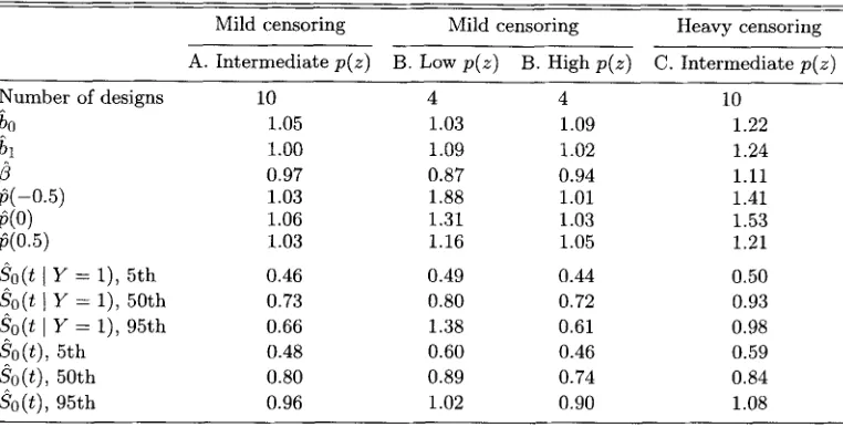
Table 1

Mean of the relative MSE (MSE( Weibull)/MSE(PH)) of

60,

b l ,

,8,

p ( z ) ,

&(t

I

Y = l ) , and

& ( t )

at percentiles comparing Weibull to P H over designs Mild censoring Mild censoring Heavy censoring A. Intermediate p ( z ) B. Low p ( z ) B. High p ( z ) C. Intermediate p ( z )

Number of designs 10 4 4 10

bo

1.05 1.03 1.09 1.22

P

0.97 0.87 0.94 1.11

p ( 0 . 5 ) 1.03 1.16 1.05 1.21

1.00 1.09 1.02 1.24

@( -0.5) 1.03 1.88 1.01 1.41

P(0) 1.06 1.31 1.03 1.53

So(t 1

Y = l ) , 5th 0.46 0.49 0.44 0.50

S o ( t 1

Y = l ) , 50th 0.73 0.80 0.72 0.93

S o ( t I

Y = l), 95th 0.66 1.38 0.61 0.98

Soot), 5th 0.48 0.60 0.46 0.59

S o o t ) ,

50th 0.80 0.89 0.74 0.84

Soot),

95th 0.96 1.02 0.90 1.08

In summary, when the true model is a Weibull mixture, un- der ideal conditions of sufficient follow-up and mild censoring, the PH mixture is comparable in efficiency in the estimation of the incidence parameters but is less efficient for the pa- rameters of the conditional survival distribution. But when censoring is heavy, the PH mixture model gets an upper hand in the incidence parameters and at times even does better with the latency parameters because of the constraint.

The coverage rates (not shown) for bo and bl are reasonable and comparable between the PH and Weibull mixture. For

0,

there can be undercoverage for both models but more often with the Weibull, mostly for designs with heavy censoring or small p ( z ) . The undercoverage is due t o underestimation in the variance of /3.

Comparisons between the observed and estimated variabili- ty of bo, b l , and ,B are simikar in tee PH and Weibull mixture. The estimated variance of bo and bl generally agrees with the observed variance when censoring is mild but i s muchA smaller when censoring is heavy. The estimated variance of ,B is gen- erally less than the observed variance, and the discrepancy becomes greater for small p ( z ) or heavy censoring.

We observed that, for low pi.) when there are only a few events observed, the estimate

0

becomes unstable, and this gets reflected in a large estimated and observed variance. We also need a reasonable proportion of the nonsusceptibles t o survive censoring t o near the end of the follow-up period in order to get a reasonable estimate of the incidence propor- tion. We find that the Weibull mixture is more sensitive t o the effects of small p ( z ) and heavy censoring because it does not get the help the PH mixture model does from the con- straint, which helps in stabilizing the tail of So(t

I

Y = 1) and improves the parameter estimates.

6. Radiation Therapy for Tonsil Cancer

The data consist of 672 patients from nine institutions world- wide (Withers et al., 1995). The subjects had squamous cell carcinoma of the tonsil and were treated with radiation dur- ing 1976-1985. The purpose of the study was to investigate

the effects of different radiation treatment regimens on local cancer control. In this example, local recurrence is defined as the event and failure time is time from initial treatment to local recurrence. Six covariates are considered: T stage (cate- gorical) with levels T1, T2, T3, T4; node status (binary), with level zero for having negative neck nodes (NO) and level one for having at least one positive node

(N+);

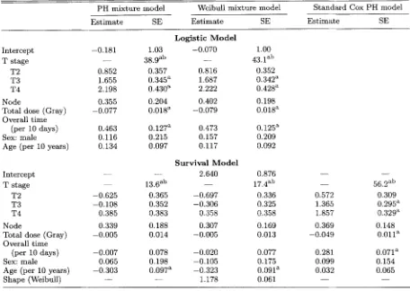
total dose (contin- uous); overall treatment duration (continuous); sex (binary); and age (continuous). All covariates are included in both parts of the model. A przorz, we might expect the T stage, node status, and treatment variables t o be more important for the incidence part of the model because incidence is directly de- termined by whether or not all the cancer cells are killed. If age is t o be important, it may influence the latency part be- cause the time t o recurrence is determined by the growth rate of the surviving tumor cells, which is potentially determined by patient specific factors such as age. Of the 672 subjects, 206 had cancer recurring. The observed follow-up time ranged from 19 days to 14.5 years. The last three recurrences were at 4.9, 5.1, and 8.2 years from initial treatment. Of the 466 cen- sored observations, 89 were censored after the last event and 126 between the last two events. A K-M plot for the whole data set has a level region beyond about 3 years, which to- gether with the biology of this tumor is a clear indication of the appropriateness of a cure model. There were 170 distinct event times, 31 with ties, and the number of ties ranged from 2 to 5. The log{- log S ( t ) } plots of the K-M survival curves against log-time for most covariates show approximately par- allel curves, but not necessarily straight lines, across covariate levels, indicating that a standard PH model might provide a reasonably good fit t o the observable marginal survival curves while a standard Weibull model might not. [image:5.594.104.485.105.298.2]

Table 2

Results from the PH mixture model, Weibull mixture model, and standard Cox PH model

PH mixture model Weibull mixture model Standard Cox PH model

Estimate SE Estimate SE Estimate SE

Intercept T stage T2 T 3 T4 Node

Total dose (Gray) Overall time

(per 10 days) Sex: male

Age (per 10 years)

Intercept T stage T2 T3 T4 Node

Total dose (Gray) Overall time

(per 10 days) Sex: male

Age (per 10 years) Shape (Weibull) -0.181 0.852 1.655 2.198 0.355 - -0.077 0.463 0.116 0.134 - - -0.625 -0.108 0.385 0.339 -0.005 -0.007 0.065 -0.303 - Logistic Model

1.03 -0.070

38.gab __

0.357 0.816

0.345” 1.687 0.430” 2.222

0.204 0.402

0.018” -0.079 0.127” 0.473 0.215 0.157

0.097 0.117

Survival Model

__ 2.640

0.365 -0.697 0.352 -0.306

13.6”b -

0.383 0.358 0.188 0.307 0.014 -0.005 0.078 -0.020 0.198 -0.105 0.097” -0.323

- 1.178

1.00 43.1”” 0.352 0.342” 0.428“ 0.198 0.018” 0.125” 0.209 0.092 0.876 17.4ab 0.336 0.325 0.358 0.169 0.013 0.077 0.175 0.091” 0.061 - - 0.572 1.365 1.857 0.369 -0.049 0.281 0.099 0.032 - - 56.2”b 0.309 0.295” 0.32ga 0.148 0.011” 0.071” 0.154 0.065 -

”p-value

<

0.01. Wald

x 2

with 3 d.f.

for sex, all the covariates are significant in at least one effect. The LRT and Wald test agree quite well.

Table 2 gives the results for the PH and Weibull mixture models and the standard Cox PH model. T stage is significant on both incidence and latency. There is more probability of local recurrence with higher stage. The effect on recurrence time is, however, not monotonic. Node is marginally signifi- cant on both incidence and latency, with a higher recurrence rate and earlier recurrence times for those with positive nodes. Total dose and overall treatment duration are very significant on incidence but not on latency. A higher total dose lowers the risk of recurrence, while a longer duration results in a higher recurrence rate. Sex is neither significant on incidence nor la- tency. Age is not significant on incidence but is significant on latency. The positive estimate for by indicates a higher, though nonsignificant, recurrence rate for older patients, but the significant negative estimate for

&

indicates later recur- rence times for older patients. This has a plausible biological explanation and is an example of marginal survival curves that cross. The results from the Weibull mixture model are mostly similar. The standard errors are not much different be- tween the PH and Weibull mixture models. The results from the standard Cox PH model agree with those for the PH mix- ture model’s global test for @ , & ) = 0 except for age. The

mixture model results in Table 2 use the zero-tail constraint. The parameter estimates obtained without this constraint are very similar, but not identical, t o those in the table.

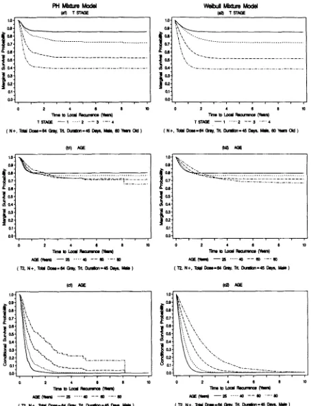
To compare the fits from the PH and Weibull mixture mod- els, we construct curves for S ( t

\

Y = 1; 2) and

S ( t ;

2) for se- lected values of z . Figure 1 compares the estimated marginal survival curves and the estimated conditional survival curves for T stage and age. The fits from the PH and Weibull mod- els are very similar for the marginal curves, while they can be different for the conditional curves, especially near the tails of the curves, although the ordering of the curves is the same. The estimated curves from PH mixture model for age at 80 years show a big jump at the tail. This is caused by the last event, which is a late event whose effect on the baseline con- ditional survival function is to shift it upward at the tail. Ex- cluding this observation reduces the jump size significantly. The plots for age show how and where the curves cross and illustrate the opposite effects of age on incidence and latency. This explains why the standard PH model was not able to detect an effect of age.

7. Discussion

[image:6.594.65.521.96.420.2]

Estimation in a Cox Proportional Hazards Cure Model

233

1 0

0 2 4 8 8 0 2 4 8 8 to

0.0 O ' l j

1.0

[image:7.594.63.517.69.661.2]

---_____

---_

Figure 1. Estimated marginal survival curves from the PH mixture model and the Weibull mixture model for

model. For each covariate, there are two parameters, one de- scribing how the covariate affects long-term incidence and one describing how it affects latency. Neither of these has the same interpretation as the relative hazard in a Cox rnodel. A covari- ate that is important for incidence may not be important for latency and vice versa. In the tonsil cancer application, the eventual cure (i.e., incidence) is of more scientific interest than when the tumor recurred (i.e., latency). The data set also pro- vides examples of variables that are important for incidence but not for latency (e.g., dose and treatment duration) and vice versa (e.g., age). This feature of the model that covariates can influence both the incidence and the latency allows more flexible modeling but also opens up the possibility of overpa- rameterization. The relative importance of the two aspects of the model may differ between applications. In our experience, the incidence part of the model is usually of more scientific interest, in which case a minimal number or no covariates in the latency part may be appropriate.

An important issue in cure models is goodness-of-fit. It is possible that, even in a cure model, a marginal P H model may hold, although this did not happen for the tonsil cancer data because of the effect of age. There are a number of ways that one might address whether a cure model is appropriate, the most important of which is having a biological rationale from the underlying science. The standard P H model is a special case of the PH cure model, with an infinitely large intercept in the logistic part. For our data, the estimate and standard error for the intercept are -0.18 and 1.03, respectively, not supporting the standard PH model. For assessing the appro- priateness of specific submodels, one could borrow ideas from standard approaches for these models. For example, for a ma- jor categorical variable, one could graphically examine a plot of log(- log((S(t) - (>

-$))I$))

versus time for each level of the variable, where S ( t ) is the estimated marginal distribu- tion and ?; is the estimated final level of the Kaplan-Meier curve. Approximately parallel lines would support the PH as-

sumption for the conditional distribution.

An alternative potential approach t o assessing the need for a cure model is to extend the ideas in Maller and Zhou (1996), who developed a method in the one-sample, no-covariate para- metric model setting. They showed that a likelihood ratio test of the no-cure model versus cure model has, asymptot- ically, a mixture of chi-squared distributions. For the Kuk and Chen (1992) model, a likelihood ratio test could be con- structed by fitting both the full model and a restricted model with p ( z ) = 1 for all z. Then an empirical estimate of the sampling distribution of the statistic could be obtained by simulating observations from the restricted model.

The semiparametric logistic-PH mixture niodel with covari- ates is identifiable for the parameters in the incidence proba- bility and the conditional survival distribution. But by leaving the conditional baseline survival function arbitrary, a condi- tion close t o nonidentifiability can occur, which causes es- timation problems. The constraint that sets the conditional survival function t o zero beyond the last event time plays a crucial role in the procedure; it is effectively eliminating the near nonidentifiability, leading to a vastly more regular likelihood surface and good properties in the estimators. The constraint could also be viewed as an alteration of the model, e.g., t o a rnodel in which there is a finite time TTllar after

which events can never occur. Then our zero-tail constraint is implicitly estimating Tmas by the largest event time. This is not unreasonable except in situations where there is poor follow-up beyond the period when events occur. Thus, this alteration to the model seems quite natural and appropriate t o us except in situations where the cure model should not be used anyway.

The estimation method proposed in this paper is a gen- eralization of the method of Taylor (1995) in his logistic K- M model where the conditional survival function does not depend on covariates. We simply set ,B = 0 and our b and

So(t

1

Y = 1) reduce t o his estimators. Statistical inference

for b in Taylor (1995) was performed using likelihood ratio tests, and no standard errors were given. A special case of the information matrix given in the Appendix of the current paper can be used t o find standard errors for the model con- sidered by Taylor (1995).

Kuk and Chen (1992) in their estimation method for this model applied a marginal likelihood approach and eliminated

So(t

I

Y = I ) by simulating the Y values of the censored

individuals. Their method effectively simulates Y = 1 or 0 with probability 112, ignoring the covariates and censoring times. They first maximize a Monte Carlo approximation of the marginal likelihood that is free of So(t

I

Y = 1) to es- timate (b,,B). Given

( k , , d ) ,

So(t

1

Y = 1) is then estimated using the nonparametric observed likelihood in an EM algo- rithm. The second step is similar to our method except that we jointly estimate ( b , p ) together with

So(t

1

Y

= 1) within the same EM algorithm. We note that their method requires repeated application of the procedure in order t o obtain the standard errors of the estimates. Furthermore, in their two- sample simulation study, it appears that their method tends t o overestimate the incidence proportion for the group with more censored observations.

ACKNOWLEDGEMENTS

This research was performed when Drs Sy and Taylor were at the Department of Biostatistics, University of California-Los Angeles, and was supported by grants CA72495 and CA16042 from the National Cancer Institute.

RESUMB

Certaines donnkes de survie peuvent Ctre issues d’une popula- tion comportant un mdlange de sujets susceptibles et de sujets non susceptibles de dkvelopper un Cvdnement d’intkr6t. Ces donnges se presentent typiquement avec un taux de censure klevk a la fin de l’ktude et une analyse standard ne sera pas toujours adaptke. Dans de telles situations o h l’on a de fortes presomptions scientifiques ou empiriques quant 8. l’existence d’une proportion de sujets non susceptibles, un modkle de melange ou de gukrison peut 6tre utilisk (Farewell, 1982). Ce modhle assume une distribution de Bernouilli pour modkliser la probabilitk d’6tre susceptible et un modble paramktrique pour la distribution des temps d’Bv6nements. Kuk et Chen (1992) ont ktendu ce modele en utilisant un modble semi- paramktrique de regression de Cox pour la distribution des dklais de survenue de l’Bv6nement. Nous ddveloppons des pro- cedures du maximum de vraisemblance, pour l’estimation jointe de l’incidence et des parametres de rkgression relative B

Estimation in a Cox Proportional Hazards Cure Model

235

kviter un problgme de non-identifiabilitb. L’inverse de la ma-

APPENDIX

trice d’information observke est utiliske pour le calcul des

Ccarts types. Une Btude de simulation montre que cette mk- thode est compktitive par rapport aux mkthodes paramktri- ques sous des conditions idkales, et est gBn6ralement plus per- formante quand la censure due aux perdus de vue est impor- t a n k . Les mkthodes SOnt aPPliqukes des donnkes de Pa- tients atteints d’un cancer de l’amygdale et trait& par ra- diothkrapie.

Observed Information Matrix

The first derivatives of the observed data log-likelihood can be obtained directly from (7). An easier, alternative way is t o use the complete-data log-likelihood from the EM algorithm and derive the function using the method of ~~~i~ (1982). Let

REFERENCES

Andersen, P. K. and Gill, R. D. (1982). Cox’s regression model for counting processes:

A

large sample study. Annals of

Statistics 10, 1100-1120.

Bailey,

K.

R. (1984). Asymptotic equivalence between the Cox

estimator and the general ML estimators of regression and survival parameters in the Cox model. Annals of

Statistics 12, 730-736.

Breslow, N. E. (1972). Contribution to the discussion of D. R. Cox (1972). Journal of the Royal Statistical Society,

Series B 34, 216-217.

Farewell,

V.

T . (1982). The use of mixture models for the analysis of survival data with long-term survivors. Bio-

metrics 38, 1041-1046.

Farewell,

V.

T . (1986). Mixture models in survival analysis: Are they worth the risk? Canadian Journal of Statistics

Kalbfleisch, J. D. and Prentice, R. L. (1980). The Statistical

Analysis of Failure Time Data. New York: Wiley.

Klein, J. P. (1992). Semiparametric estimation of random ef- fects using the Cox model based on the EM algorithm.

Biometrics 48, 795-806.

Kuk, A. Y. C. and Chen, C. H. (1992). A mixture model combining logistic regression with proportional hazards regression. Biometrika 79, 531-541.

Louis, T . A. (1982). Finding the observed information ma- trix when using the EM algorithm. Journal of the Royal

Statistical Society, Series B 44, 226-233.

Maller, R. A . and Zhou, S. (1996). Survival Analysis with Long

Term Survivors. New York: Wiley.

Peng, Y., Dear, K . B. G., and Denham, J. W. (1998). A gener- alized F mixture model for cure rate estimation. Statis-

14, 257-262.

and

The components of the score function are

i = l ,

. . . ,

k ,

where

for 1 censored and w1 = 1 for 1 uncensored and h o ( t l

I

Y =

tics in Medicine 17, 813-830.

I)

=

c .

J : t ( , l l t l X j . The observed information matrix I ( b , /3, A)

has components Prentice, R. L. and Gloeckler, L. A. (1978). Regression anal-

ysis of grouped survival data with application t o breast _n n

d2

-- logL = c x l z ; p L ( l - p i ) - C z 1 z ; w 1 ( 1 - wz)

cancer data. Biometrics 34, 57-67.

Sy, J . P. and Taylor, J. M. G. (1999). Standard errors for the Cox proportional hazards curve model. Mathematical

Taylor, J. M. G. (1995). Semi-parametric estimation in failure Tsiatis, A. A. (1981). A large sample study of Cox’s regression

1=1 1=1

ab2

k

and Computer Modelling, in press.

a2

aP2

-- logL = Xi w l z l z l e z ’ P

zlzihil (1 - e-hti - h a1 e-htl

1

i=l l E R i

time mixture models. Biometrics 51, 899-907.

model. Annals of Statistics 9, 93-108. ₂

Withers, H. R., Peters, L. J., Taylor, J. M. G., et al. (1995). Local control of carcinoma of the tonsil by radiation ther-

i = l LED,

n

apy: An analysis of patterns of fractionation in nine in- - E w l ( 1 - w l ) z l z [ {e’;’Ao(tl

I

Y =

stitutions. International Journal of Radiation Oncology, 1=1

Biology, Physics 33, 549-562.

a2

--logL=

axq

c

- e-h’L) 2

ED,

Received March 1997. Revised March 1999.

x I (tl

L

t ( % ) )

I (tl

2

t ( , ) )

7

#

j , z = l ,

. . . ,

k , --

”

log L =

2

wl(1 - wl)zlz;e”lPAg(tl

I

Y = 1)

a b a p

where h,l = A, exp(ziP). Note that

-a2

log L/db2,

-a2

log L/

ap2,

-a2

log L/aA2, and

-6’’

log LlapaA, have analogous ex- pressions in the standard logistic regression and PH model except for negative terms for censored observations that in- volve w l ( l - w l ) , which reflects the variability in the estimated weights. When the constraint S o ( t ( k )

I

Y = 1) = 0 is imposed, then a k = 0 and = cm and the dimension of A is reduced to

t

- 1.

1=1

-- d2 logL =

c

Wl(1 - W l ) Z & P ,

-- a2 logL =

c

wlzlez;P

2 = 1 , .

. . ,

Ic,

dbaAa l E R ,

l E R ,