Split hierarchical variational inequality problems and fixed point problems for nonexpansive mappings

R E S E A R C H

Open Access

Split hierarchical variational inequality

problems and fixed point problems for

nonexpansive mappings

Qamrul Hasan Ansari

_{, Aisha Rehan}

_{and Ching-Feng Wen}

*_{Correspondence:} [email protected]

2_{Center for Fundamental Science,} Kaohsiung Medical University, Kaohsiung, 807, Taiwan, ROC 3_{Center for Nonlinear Analysis and} Optimization, Kaohsiung Medical University, Kaohsiung, 807, Taiwan, ROC

Full list of author information is available at the end of the article

Abstract

The present paper deals with the common solution method for finding a fixed point of a nonexpansive mapping and a solution of split hierarchical Minty variational inequality problems. We discuss the weak convergence of the sequences generated by the proposed method to a common solution of a fixed point problem and a split hierarchical Minty variational inequality problem. An example is presented to illustrate the proposed algorithm and result.

MSC: 49J40; 49J52; 47J20

Keywords: split hierarchical variational inequality problems; fixed point problems; iterative method; nonexpansive mappings; convergence analysis

1 Introduction

Since its origin in  by Censor and Elfving [], thesplit feasibility problem(SFP) has been rapidly investigated and studied because of its applications in different areas such as signal processing, phase retrievals, image reconstruction, intensity-modulated radiation therapy,etc.(see, for example, [–] and the references therein). Recently, Censor and Se-gal [] introduced asplit common fixed point problem(SCFPP) which is to find a common element of a family of operators in one space such that its image under a linear transfor-mation is a common fixed point of another family of operators in the image space. The SCFPP generalizesconvex feasibility problem(CFP), split feasibility problem(SFP) and multiple sets split feasibility problem(MSSFP). They developed a parallel algorithm for solving SCFPP for the class of directed operators in the setting of finite-dimension spaces. Further, Cuiet al.[] proposed a damped projection method for SCFPP and studied its convergence result. Moudafi [] further proposed and analyzed an iterative scheme for solving SCFPP for the class of demicontractive operators in the setting of Hilbert spaces. He studied the weak convergence of the sequence generated by the proposed algorithm to a solution of SCFPP. Subsequently, Cui and Wang [] suggested a new algorithm that does not require any prior information of the operator norm to find a solution of SCFPP. They studied the weak convergence of the proposed algorithm. In , Moudafi [] con-sidered the relaxed algorithm for computing the approximate solution of SCFPP for quasi-nonexpansive operators and studied the weak convergence of the sequence generated by the suggested algorithm. Very recently, SCFPP was considered by Kraikaew and Saejung

[] for quasi-nonexpansive and strongly quasi-nonexpansive operators. They proposed an algorithm and showed that their algorithm converges strongly to a solution of SCFPP. They also considered split variational inequality problem[],split common null point problemandMoudafi’s split feasibility problem, and derived the algorithm for these prob-lems from the main algorithm for SCFPP. Also, the strong convergence of these algorithms is derived from the main convergence result. Very recently, Ansariet al.[] introduced the split hierarchical variational inequality problem(SHVIP). A variational inequality prob-lem in which the underlying set is a set of fixed points of a nonlinear operator is called hierarchical variational inequality problem. For further details on hierarchical variational inequality problems, we refer to [] and the references therein. More precisely, they con-sidered the followingsplit hierarchical Minty variational inequality problem(SHMVIP) which requires to find a solution of ahierarchical Minty variational inequality problem (HMVIP) such that its image under a nonlinear operator is a solution of another HMVIP. LetHandHbe real Hilbert spaces,f,T:H→Hbe operators such thatFix(T)=∅, andh,S:H →H be operators withFix(S)=∅, whereFix(T) andFix(S) are denoted by the set of fixed points ofT andS, respectively. LetA:H→H be an operator with R(A)∩Fix(S)=∅, whereR(A) denotes the range ofA. Thesplit hierarchical variational inequality problem(SHVIP) is to findx∗∈Fix(T) such that

fx∗,x–x∗≥ for allx∈Fix(T) () such thatAx∗∈Fix(S) and it satisfies

hAx∗,y–Ax∗≥ for ally∈Fix(S). () The solution set of the SHVIP is denoted by.

Another problem which is closely related to (SHVIP) is the followingsplit hierarchical Minty variational inequality problem(SHMVIP): Findx∗∈Fix(T) such that

f(x),x–x∗≥ for allx∈Fix(T), () and such thatAx∗∈Fix(S) satisfies

h(y),y–Ax∗≥ for ally∈Fix(S). ()

We denote bythe set of solutions of SHMVIP, that is,

=xsolves () :Axsolves ().

It can be easily seen by the Minty lemma [], Lemma , that ifFix(T) andFix(S) are nonempty closed convex andf andhare monotone and continuous, then SHVIP ()-() and SHMVIP ()-() are equivalent.

In this paper, we give a common solution method for finding a fixed point of a nonex-pansive operator and a solution of split hierarchical variational inequality problems. The weak convergence of such algorithm is studied. We also present an example to illustrate the proposed algorithm and the convergence result.

2 Preliminaries

LetH be a real Hilbert space whose inner product and norm are denoted by ·,·and

· , respectively. LetCbe a nonempty closed convex subset ofH. We denote byxn→x (respectively,xnx) the strong (respectively, weak) convergence of the sequence{xn}to x. LetT:H→Hbe an operator whose range is denoted byR(T). The set of all fixed points ofTis denoted byFix(T), that is,Fix(T) ={x∈H:x=Tx}.

Definition . An operatorT:H→His said to be: (a) nonexpansiveifTx–Ty ≤ x–yfor allx,y∈H; (b) strongly nonexpansive[, ] ifTis nonexpansive and

lim

n→∞(xn–yn) – (Txn–Tyn)= ,

whenever{xn}and{yn}are bounded sequences inHand lim_n→∞(xn–yn–Txn–Tyn) = ;

(c) averaged nonexpansiveif it can be written as

T= ( –α)I+αS,

whereα∈(, ),Iis the identity operator ofH, andS:H→His a nonexpansive mapping;

(d) firmly nonexpansiveifTx–Ty_{≤ x–y,Tx–Tyfor allx,y∈H;} (e) cutter[] if x–Tx,z–Tx ≤for allx∈Handz∈Fix(T); (f ) monotoneif x–y,Tx–Ty ≥for allx,y∈H;

(g) α-inverse strongly monotoneif there exists a constantα> such that

Tx–Ty,x–y ≥αTx–Ty for allx,y∈H.

Remark . Every strongly nonexpansive operator is nonexpansive, but a nonexpansive operator need not be strongly nonexpansive. Also, a nonexpansive cutter operator need not be strongly nonexpansive.

Example . LetT: [–, ]→Rbe defined byTx= –xfor allx∈[–, ]. ThenT is non-expansive but not strongly nonnon-expansive.

Indeed, letxn=  andyn=  for alln. Then{xn}and{yn}are bounded sequences. Also,

lim

n→∞ (xn–yn) – (Txn–Tyn) =nlim→∞| + |= = .

Thus,Tis not strongly nonexpansive.

x ≤√}be a nonempty closed subspace ofR_{. LetT:C→Cbe defined by}

T(x,y) =

 x+

 y,

 x+

 y

for all (x,y)∈C.

ThenT is a nonexpansive cutter operator, butTis not strongly nonexpansive.

Indeed, let{xn}= (, ) and{yn}= (, ) for alln. Then{xn}and{yn}are two bounded sequences ofC, andTxn= (_,_) andTyn= (, ). Note that

lim n→∞

xn–yn–Txn–Tyn = lim n→∞ (, )–  ,   = lim

n→∞( – ) = . But

lim

n→∞(xn–yn) – (Txn–Tyn)=nlim→∞ (, ) –  ,   = lim n→∞ _,–  = = .

Thus,Tis not strongly nonexpansive.

In order to show thatTis a nonexpansive cutter operator, we first prove that it is non-expansive. Letx= (x,x),y= (y,y)∈C. Then

Tx–Ty=

 x+

 x,

 x+

 x

–

 y+

 y,

 y+

 y

=

(x–y) + 

(x–y), 

(x–y) + 

(x–y)

= 

(x–y) + 

(x–y) + 

(x–y) + 

(x–y)

≤

|x–y|+ 

|x–y|+ 

|x–y|+ 

|x–y|

=|x–y|+|x–y|=(x–y), (x,y)

=(x,x) – (y,y)=x–y.

Thus,Tis nonexpansive.

We next show thatT is cutter. Note thatFix(T) ={(x,y)∈C:x=y}. Letx= (x,y)∈C and (p,p)∈Fix(T), we have

x–Tx,p–Tx=

(x,y) –

 x+

 y,

 x+

 y

, (p,p) –

 x+

 y,

 x+

 y =  (x–y),

 (y–x)

,

p–

(x+y),p–  (x+ y)

= (x–y)

p–

(x+y)

+ (y–x)

p–

(x+ y)

= (x–y)

p– (x+y) – p+ (x+ y)

=

(x–y)(y–x) = –  (x–y)

_≤.

The following lemma provides some fundamental properties of Hilbert spaces. These properties will be used in the sequel.

Lemma . Let H be a real Hilbert space.Then,for all x,y∈H,we have (a) x–y=x–y– x–y,y;

(b) x–y_{≤ x}_{+ y,y–x;}

(c) λx+ ( –λ)y_=λx_{+ ( –λ)y}_{–λ( –λ)x–y}_{for allλ∈[, ].}

Lemma .([], Lemma , Demiclosedness principle) Let C be a nonempty closed con-vex subset of a real Hilbert space H and T :C→C be a nonexpansive operator with

Fix(T)=∅.If the sequence {xn} ⊆C converges weakly to x and the sequence{(I–T)xn} converges strongly to y,then(I–T)x=y;in particular,if y= ,then x∈Fix(T).

Definition . LetT :H→H _{be a set-valued operator with domainD(T) ={x∈H:} T(x)=∅}, rangeR(T) =_x∈D(T)T(x) and the inverse ofT isT–(y) ={x∈H:y∈T(x)}. T is said to be:

(a) monotoneif

x–y,f–g ≥, wheneverf∈Tx,g∈Ty;

(b) maximal monotoneif it is monotone and the graph

G(T) =(x,f)∈H×H:f ∈Tx

ofTis not properly contained in the graph of any other monotone operator; (c) α-inverse strongly monotoneif there exists a constantα> such that

Tx–Ty,x–y ≥αTx–Ty, wheneverx,y∈D(T).

It is well known that whenTis maximal monotone, then for eachx∈Handλ> , there is a uniquez∈H such thatx∈(I+λT)z. In this case, the operatorJλT:= (I+λT)–is

called resolvent ofT with parameterλ. It is known thatJT

λ is a single-valued and firmly

nonexpansive mapping.

The following lemma will be used in our main result.

Lemma .([]) Let{an}∞n=and{bn}∞n=be sequences of nonnegative real numbers such that

an+≤an+bn for all n≥.

If∞_n=bn<∞,then the limitlimn→∞anexists.

3 Algorithms and convergence results

Algorithm . Initialization: Choose{αn}∞n=,{βn}∞n=,{λn}∞n=⊂(, ). Take arbitrary x∈H.

Iterative step: For a given currentxn∈H, compute

zn=xn–γA∗

I–S(I–βnh)

Axn,

yn=T(I–αnf)zn,

xn+=λnxn+ ( –λn)Kyn,

()

whereγ ∈(,_A).

Last step: Updaten:=n+ .

WhenKis the identity operator, Algorithm . reduces to the following algorithm.

Algorithm . Initialization: Choose{αn}∞n=,{βn}∞n=,{λn}∞n=⊂(, ). Take arbitrary x∈H.

Iterative step: For a given currentxn∈H, compute

zn=xn–γA∗

I–S(I–βnh)

Axn,

yn=T(I–αnf)zn,

xn+=λnxn+ ( –λn)yn,

()

whereγ ∈(,_A).

Last step: Updaten:=n+ .

Next we prove the weak convergence of the sequences generated by Algorithm ..

Theorem . Let f :H→Hbe a monotone continuous mapping,T:H→Hbe a non-expansive cutter operator such thatFix(T)=∅, h:H→H be a monotone continuous mapping and S:H→Hbe a strongly nonexpansive cutter operator such thatFix(S)=∅. Let A:H→Hbe a bounded linear operator with R(A)∩Fix(S)=∅and let K:H→Hbe a nonexpansive operator withFix(K)∩=∅.Let{xn}and{yn}be the sequences generated by Algorithm.such that the following conditions hold:

(i) There exists a natural numbern◦such that

⊂

∞

n=n◦

z∈H:h(Axn),S(I–βnh)Axn–Az

≥;

(ii) {f(zn)}∞n=is a bounded sequence; (iii) ∞_n=αn<∞;

(iv) limn→∞βn= ;

(v) xn+–xn=o(αn)andαn=o(βn); (vi) {h(Axn)}∞n=is a bounded sequence.

Proof Letp∈Fix(K)∩. ThenT(p) =p,K(p) =pandS(Ap) =Ap. Consider

zn–p=xn–γA∗

I–S(I–βnh)

Axn–p

=xn–p+γA∗

I–S(I–βnh)

Axn

– γxn–p,A∗

I–S(I–βnh)

Axn

≤ xn–p+γAI–S(I–βnh)

Axn

– γxn–p,A∗

I–S(I–βnh)

Axn

for alln≥. ()

SinceSis a cutter operator, we have

xn–p,A∗

S(I–βnh) –I

Axn

=Axn–Ap,

S(I–βnh) –I

Axn

=S(I–βnh)Axn–Ap+Axn–S(I–βnh)Axn,

S(I–βnh) –I

Axn

=S(I–βnh)Axn–Ap,

S(I–βnh) –I

Axn

–S(I–βnh) –I

Axn 

=S(I–βnh)Axn–Ap,

S(I–βnh) –I

Axn+βnhAxn–βnhAxn

–S(I–βnh) –I

Axn

=S(I–βnh)Axn–Ap,S(I–βnh)Axn– (I–βnh)Axn

–βn

S(I–βnh)(Axn) –Ap,h(Axn)

–S(I–βnh) –I

Axn 

≤–S(I–βnh) –I

Axn 

–βn

S(I–βnh)(Axn) –Ap,h(Axn)

.

Sincep∈, by condition (i), we have

S(I–βnh)(Axn) –Ap,h(Axn)

≥.

Sinceβn∈(, ) for alln∈N, we further have

βn

S(I–βnh)(Axn) –Ap,h(Axn)

≥.

Therefore,

xn–p,A∗

S(I–βnh) –I

Axn

≤–S(I–βnh) –I

Axn 

.

Thus, () becomes

zn–p≤ xn–p+γAI–S(I–βnh)

Axn 

– γS(I–βnh) –I

Axn 

=xn–p–γ

 –γAS(I–βnh) –I

Axn for alln≥. ()

Sinceγ∈(, 

A), we observe thatγ( –γA) > , and hence

LetM:=sup{f(zn):n≥}. Then, for alln≥, we have

yn–p=T

zn–αnf(zn)

–T(p)

≤ zn–p+αnf(zn)

≤ zn–p+αnM

≤ xn–p+αnM, ()

xn+–p=λnxn+ ( –λn)Kyn–p

=λn(xn–p) + ( –λn)(Kyn–p)

≤λnxn–p+ ( –λn)yn–p

≤λnxn–p+ ( –λn)xn–p+ ( –λn)αnM

≤ xn–p+ ( –λn)αnM.

Sinceαn<∞and  < ( –λn) < , we have _∞

n=( –λn)αn<∞. Thus, by Lemma ., the limit limn→∞xn–p exists. Also, from ()-(), the limits limn→∞zn–p and limn→∞yn–pexist. This implies that{xn},{yn}and{zn}are bounded sequences. Now, consider

yn–p=T(I–αnf)(zn) –T(p)

≤(zn–p) –αnf(zn)

≤ zn–p+αnf(zn) 

. ()

From (), () and by Lemma .(c), we have

xn+–p =λnxn+ ( –λn)Kyn–p

=λn(xn–p) + ( –λn)(Kyn–p)

=λnxn–p+ ( –λn)yn–p–λn( –λn)Kyn–xn

≤λnxn–p+ ( –λn)

zn–p+αnf(zn)

–λn( –λn)Kyn–xn

≤λnxn–p+ ( –λn)xn–p

– ( –λn)γ

 –γAS(I–βnh) –I

Axn

+ ( –λn)αnf(zn)–λn( –λn)Kyn–xn

=xn–p– ( –λn)γ

 –γAS(I–βnh) –I

Axn

+ ( –λn)αnf(zn)–λn( –λn)Kyn–xn, ()

which is equivalent to

( –λn)γ

 –γAS(I–βnh) –I

Axn 

+λn( –λn)Kyn–xn

≤ xn–p–xn+–p+ ( –λn)αnf(zn) 

From the existence of the limit limn→∞xn–p and the facts thatαn→,f(zn) is bounded,  <λn<  andγ ∈(,_A), it follows that

lim

n→∞S(I–βnh) –I

Axn= , ()

and

lim

n→∞Kyn–xn= . ()

From (), we have

lim

n→∞xn+–xn ≤nlim→∞Kyn–xn= . ()

SinceTis a cutter operator, we have

p–yn,zn–yn

= yn–p,yn–zn

=T(I–αnf)zn–p,T(I–αnf)zn– (I–αnf)zn+ (I–αnf)zn–zn

=T(I–αnf)zn–p,T(I–αnf)zn– (I–αnf)zn

+T(I–αnf)zn–p, –αnfzn

≤T(I–αnf)zn–p,T(I–αnf)zn– (I–αnf)zn

+αnT(I–αnf)zn–pfzn,

and

T(I–αnf)zn–p,T(I–αnf)zn– (I–αnf)zn

≤.

This implies that

p–yn,zn–yn ≤αnT(I–αnf)zn–pfzn. ()

From (), () and by Lemma .(a), we have

yn–p =zn–p–zn–yn– yn–p,zn–yn

≤ xn–p–xn–γA∗

I–S(I–βnh)

Axn–yn

–  yn–p,zn–yn

=xn–p–xn–yn–γAI–S(I–βnh)

Axn 

+ γxn–yn,A∗

I–S(I–βnh)Axn

+ p–yn,zn–yn

≤ xn–p–xn–yn–γAI–S(I–βnh)

Axn 

+ αnT(I–αnf)zn–pfzn

+ γxn–ynAS(I–βnh) –I

Thus, from () and (), we have

xn+–p

=λnxn–p+ ( –λn)yn–p–λn( –λn)Kyn–xn

≤λnxn–p+ ( –λn)xn–p– ( –λn)γAI–S(I–βnh)

Axn 

– ( –λn)xn–yn–λn( –λn)Kyn–xn

+ ( –λn)αnT(I–αnf)zn–pf(zn)

+ γ( –λn)xn–ynAS(I–βnh) –I

Axn

≤ xn–p– ( –λn)xn–yn– ( –λn)γAI–S(I–βnh)

Axn 

+ ( –λn)αnT(I–αnf)zn–pf(zn)–λn( –λn)Kyn–xn

+ γ( –λn)xn–ynAS(I–βnh) –I

Axn,

which is equivalent to

( –λn)xn–yn≤ xn–p–xn+–p–λn( –λn)Kyn–xn

+ ( –λn)αnT(I–αnf)zn–pf(zn)

+ γ( –λn)xn–ynAS(I–βnh) –I

Axn.

Taking limit asn→ ∞, and taking into accountαn→,  <λn< ,γ∈(,_A) and from

equations (), () we have

xn–yn → asn→ ∞, ()

yn–Kyn=yn–xn+xn–Kyn

≤ yn–xn+xn–Kyn.

From () and (), we obtain

yn–Kyn → asn→ ∞. ()

Since{xn}is a bounded sequence, there exists a convergent subsequence{xni}of{xn}that

converges weakly to somex∗∈H. Sincexn–yn →, it is known thatynix∗∈H. By

the demiclosed principle,ynix∗andyni–Kyni →, we have

Kx∗=x∗. From (), we obtain

zn–xn=γAI–S(I–βnh)

Axn.

By (), we have

and

zn–yn ≤ xn–yn+γAI–S(I–βnh)

Axn.

Equations () and () yield that

zn–yn → asn→ ∞. ()

From the definition ofyn, we have

yn–Tzn=T

zn–αnf(zn)

–Tzn

≤zn–αnf(zn) –zn

≤αnf(zn).

This implies that

lim

n→∞yn–Tzn= , ()

yn–Tyn=yn–Tzn+Tzn–Tyn

≤ yn–Tzn+zn–yn.

From () and (), we get

lim

n→∞yn–Tyn →.

Sinceynix∗andyni–Tyni →, by the demiclosed principle, we obtain

Tx∗=x∗.

Letvn:=Axn–βnh(Axn) for alln≥. We observe that

≤ vn–Ap–Svn–SAp

=Axn–βnh(Axn) –Ap–Svn–SAp

=Axn–Svn+Svn–βnh(Axn) –Ap–Svn–SAp

≤ Axn–Svn+Svn–SAp+βnh(Axn)–Svn–SAp

=Axn–S

Axn–βn

h(Axn)+βnh(Axn)

=S(I–βnh) –I

Axn+βnh(Axn).

From condition (iv) and (), we have

lim n→∞

vn–Ap–Svn–SAp

= .

The boundedness ofvnand strong nonexpansiveness ofSimply that

lim

From the definition ofvnand condition (iv), we get

lim

n→∞vn–Axn=  ()

and

vn–SAxn ≤ vn–Svn+Svn–S(Axn)

=vn–Svn+vn–Axn.

From () and (), we have

lim

n→∞vn–SAxn= , and thus

lim

n→∞Axn–SAxn= . ()

Sincexnix∗∈H, we haveAxniAx∗∈H. From () and by the demiclosed principle,

we obtain

SAx∗=Ax∗.

Letqn:=zn–αnf(zn). By Lemma .(b) and inequality (), we have

yn–p=T(I–αnf)zn–Tp 

≤zn–p–αnf(zn)

≤ zn–p+ 

αnf(zn),αnf(zn) –zn+p

=zn–p+ 

αnf(zn),p–zn

+ α_nf(zn)

≤ xn–p+ αn

f(zn),p–zn

+ α_nf(zn). ()

From the definition ofxn+, () and using the monotonicity off, we have

xn+–p≤λnxn–p+ ( –λn)yn–p

≤λnxn–p+ ( –λn)

xn–p+ αn

f(zn),p–zn

+ α_nf(zn)

≤ xn–p+ ( –λn)αn

f(zn),p–zn

+ ( –λn)αnf(zn)

=xn–p+ ( –λn)αn

f(zn) –f(p) +f(p),p–zn

+ ( –λn)αnf(zn) 

=xn–p+ ( –λn)αn

f(zn) –f(p),p–zn

+ ( –λn)αn

f(p),p–zn

+ ( –λn)αnf(zn) 

=xn–p– ( –λn)αn

+ ( –λn)αn

f(p),p–zn

+ ( –λn)αnf(zn) 

=xn–p+ ( –λn)αn

f(p),p–zn

+ ( –λn)αnf(zn) 

, ()

which is equivalent to

( –λn)

f(p),zn–p

≤

xn–p–xn+–p αn

+ ( –λn)αnf(zn)

≤

(xn–p+xn+–p)(xn–p–xn+–p) αn

+ ( –λn)αnf(zn) 

≤M

xn–p–xn+–p αn

+ ( –λn)αnf(zn)

≤M

xn–xn+ αn

+ ( –λn)αnf(zn) 

,

whereM=sup{xn–p+xn+–p,n≥}<∞. Taking limit of both sides and taking into account that  < ( –λn) < ,αn→,xn–xn+=o(αn) andznix∗, we have

f(p),x∗–p≤,

and thus

f(p),x∗–p≤ for allp∈Fix(T),

that is,x∗∈Fix(T) solves (). Sinceαn=o(βn), we may assume thatαn≤βnfor alln≥. From (), for alln≥, we have

( –λn)γ

 –γAS(I–βnh) –I

Axn

≤ xn–p–xn+–p+αnf(zn)

≤xn–p+xn+–p

xn–p–xn+–p

+α_nf(zn)

≤Mxn–xn++αnf(zn) 

,

whereM=sup{xn–p+xn+–p:n≥}<∞. Therefore, for alln≥, we have

( –λn)γ

 –γAAxn–Svn 

β n

≤xn–xn+ β

n

M+α  n

β n

f(zn)

≤xn–xn+ αn

M+αnf(zn).

Subsequently, sinceαn→,xn+–xn=o(αn),γ( –γA) >  and  < ( –λn) < , we have

lim n→∞

Axn–Svn

βn

For alln≥, by Lemma .(b) and the monotonicity ofh, we compute

Svn–SAp

≤ vn–Ap

≤Axn–βnh(Axn) –Ap 

≤ Axn–Ap+ 

βnh(Axn),βnh(Axn) –Axn+Ap

≤ Axn–Ap+ βn

h(Axn),Ap–Axn

+ β_nh(Axn) 

≤ Axn–Ap– βn

h(Ap) –h(Axn),Ap–Axn

+ β_nh(Axn) 

+ βn

h(Ap),Ap–Axn

≤ Axn–Ap+ βnh(Axn)+ βn

h(Ap),Ap–Axn

. ()

This gives

h(Ap),Axn–Ap

≤

Axn–Ap–Svn–SAp

βn

+ βnh(Axn) 

≤

(Axn–Ap–Svn–SAp)(Axn–Ap+Svn–SAp)

βn

+ βnh(Axn)

≤

Axn–Svn

βn

M+ βnh(Axn) 

,

whereM:=sup{Axn–Ap+Svn–SAp:n≥}<∞. From (), condition (iv) and AxnAp, we obtain

h(Ap),Ax∗–Ap≤ for allAp∈Fix(S),

that is,Ax∗solves (). Finally, it remains to show thatxnx∗. Note that, by the bound-edness of {xn}, it suffices to show that there is no subsequence{xni} of{xn} such that

xniy∗∈Handy∗=x∗.

Indeed, if this is not true, then the well-known Opial theorem would imply

lim n→∞xn–y

∗_=lim

j→∞xnj–x

∗_{< lim}

j→∞xnj–y

∗

= lim n→∞xn–y

∗_=lim

i→∞ xni–y

∗

< lim i→∞xni–x

∗_{= lim}

n→∞xn–y

∗_,

which leads to a contradiction. Therefore, the sequence{xn}∞n=converges weakly to a so-lutionx∗∈. Thus,xn–yn → andxn–zn → imply thatynx∗ andznx∗,

respectively.

Now, we illustrate Algorithm . and Theorem . by the following example.

Example . LetH,H,CandTbe the same as in Example .. LetS:C→Cbe defined as

S(x,y) =

 x+

 y,

 x+

 y

for all (x,y)∈C.

ThenSis strongly nonexpansive cutter and firmly nonexpansive, and it has a fixed point (, ). Thus being firmly nonexpansive,Sis strongly nonexpansive. Also, every firmly non-expansive operator with a fixed point is cutter (see [, ]). Thus,Sis a strongly nonex-pansive cutter operator.

Letf,h:C→Cbe operators defined by

f(x,y) =

 x–

 y, –

 x+

 y

for all (x,y)∈C,

and

h(x,y) =

 x–

 y, –

 x+

 y

for all (x,y)∈C.

Thenf andhare monotone. LetK:C→Cbe defined by

K(x,y) =

 x+

 y,

 x+

 y

for all (x,y)∈C.

ThenKis nonexpansive. LetA:C→Cbe defined by

A(x,y) =

 x,

 y

for all (x,y)∈C.

ThenAis a bounded linear operator andA₌ .

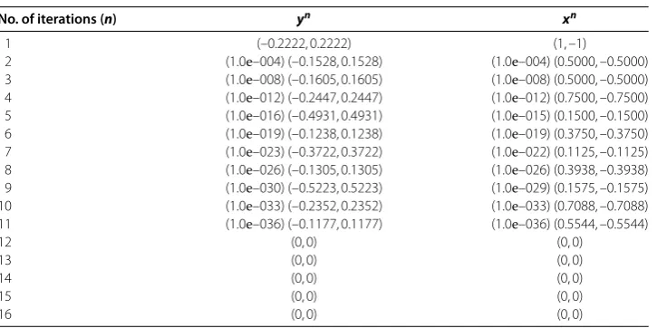
Table 1 Convergence table of Example 3.1

No. of iterations (n) yn xn

1 (–0.2222, 0.2222) (1, –1)

2 (1.0e–004) (–0.1528, 0.1528) (1.0e–004) (0.5000, –0.5000)

3 (1.0e–008) (–0.1605, 0.1605) (1.0e–008) (0.5000, –0.5000)

4 (1.0e–012) (–0.2447, 0.2447) (1.0e–012) (0.7500, –0.7500)

5 (1.0e–016) (–0.4931, 0.4931) (1.0e–015) (0.1500, –0.1500)

6 (1.0e–019) (–0.1238, 0.1238) (1.0e–019) (0.3750, –0.3750)

7 (1.0e–023) (–0.3722, 0.3722) (1.0e–022) (0.1125, –0.1125)

8 (1.0e–026) (–0.1305, 0.1305) (1.0e–026) (0.3938, –0.3938)

9 (1.0e–030) (–0.5223, 0.5223) (1.0e–029) (0.1575, –0.1575)

10 (1.0e–033) (–0.2352, 0.2352) (1.0e–033) (0.7088, –0.7088)

11 (1.0e–036) (–0.1177, 0.1177) (1.0e–036) (0.5544, –0.5544)

12 (0, 0) (0, 0)

13 (0, 0) (0, 0)

14 (0, 0) (0, 0)

15 (0, 0) (0, 0)

Letαn= (/n, /n),βn= (/n, /n),γ ∈(, ) andλn∈(, ). Then the sequencesxn andyngenerated by Algorithm . with initial guessx= (, –) converge to (, ) (see Table ) which is a fixed point ofTandK, whereasA(, ) = (, ) which is the fixed point ofS, wherex= (x,x). Thus, (, ) is the required solution.

Competing interests

The authors declare that they have no competing interests.

Authors’ contributions

All authors have equal contribution.

Author details

1_{Department of Mathematics, Aligarh Muslim University, Aligarh, India.}2_{Center for Fundamental Science, Kaohsiung} Medical University, Kaohsiung, 807, Taiwan, ROC.3_{Center for Nonlinear Analysis and Optimization, Kaohsiung Medical} University, Kaohsiung, 807, Taiwan, ROC.

Acknowledgements

In this research, the last author was partially supported by the Grant MOST 104-2115-M-037-001.

Received: 27 March 2015 Accepted: 23 August 2015

References

1. Censor, Y, Elfving, T: A multiprojection algorithm using Bregman projections in a product space. Numer. Algorithms8, 221-239 (1994)

2. Ansari, QH, Rehan, A: Split feasibility and fixed point problems. In: Ansari, QH (ed.) Nonlinear Analysis: Approximation Theory, Optimization and Applications, pp. 281-322. Springer, New York (2014)

3. Byrne, C: Iterative oblique projection onto convex subsets and the split feasibility problem. Inverse Probl.18, 441-453 (2002)

4. Byrne, C: A unified treatment of some iterative algorithms in signal processing and image reconstruction. Inverse Probl.20, 103-120 (2004)

5. Censor, Y, Bortfeld, T, Martin, B, Trofimov, A: A unified approach for inversion problems in intensity-modulated radiation therapy. Phys. Med. Biol.51, 2353-2365 (2006)

6. Ceng, L-C, Ansari, QH, Yao, J-C: An extragradient method for solving split feasibility and fixed point problems. Comput. Math. Appl.64, 633-642 (2012)

7. Ceng, L-C, Ansari, QH, Yao, J-C: Mann type iterative methods for finding a common solution of split feasibility and fixed point problems. Positivity16, 471-495 (2012)

8. Ceng, L-C, Wong, M-M, Yao, J-C: A hybrid extragradient-like approximation method with regularization for solving split feasibility and fixed point problems. J. Nonlinear Convex Anal.14, 163-182 (2013)

9. Censor, Y, Segal, A: The split common fixed point problems for directed operators. J. Convex Anal.16, 587-600 (2009) 10. Cui, H, Su, M, Wang, F: Damped projection method for split common fixed point problems. Fixed Point Theory Appl.

2013, Article ID 123 (2013)

11. Moudafi, A: The split common fixed-point problem for demicontractive mappings. Inverse Probl.26, 1-6 (2010) 12. Cui, H, Wang, F: Iterative method for the split common fixed point problem in Hilbert spaces. Fixed Point Theory

Appl.2014, Article ID 78 (2014)

13. Moudafi, A: A note on the split common fixed-point problem for quasi nonexpansive operators. Nonlinear Anal.74, 4083-4087 (2011)

14. Kraikaew, R, Saejung, S: On split common fixed-point problems. J. Math. Anal. Appl.415, 513-524 (2014) 15. Censor, Y, Gibali, A, Reich, S: Algorithms for the split variational inequality problem. Numer. Algorithms59, 301-323

(2012)

16. Ansari, QH, Nimana, N, Petrot, N: Split hierarchical variational inequality problems and related problems. Fixed Point Theory Appl.2014, Article ID 208 (2014)

17. Ansari, QH, Ceng, L-C, Gupta, H: Triple hierarchical variational inequalities. In: Ansari, QH (ed.) Nonlinear Analysis: Approximation Theory, Optimization and Applications, pp. 231-280. Springer, New York (2014)

18. Minty, GJ: On the generalization of a direct method of the calculus of variations. Bull. Am. Math. Soc.73, 314-321 (1967)

19. Bruck, RE, Reich, S: Nonexpansive projections and resolvent of assertive operators in Banach spaces. Houst. J. Math.3, 459-470 (1977)

20. Cegeilski, A: Iterative Methods for Fixed Point Problems in Hilbert Spaces. Springer, New York (2012)

21. Opial, Z: Weak convergence of the sequence of successive approximations for nonexpansive mappings. Bull. Am. Math. Soc.73, 591-597 (1976)