Driving cycle for small and medium duty engine: case study of Ipoh

CASE STUDY OF IPOH

FAUZI BIN AB GHAFAR

A project report submitted in fulfillment of the requirement for the award of the Degree of Master of Mechanical Engineering

Faculty of Mechanical and Manufacturing Engineering Universiti Tun Hussein Onn Malaysia

v

ABSTRACT

ABSTRAK

vii CONTENTS TITLE DECLARATION DEDICATION ACKNOWLEGEMENT ABSTRACT ABSTRAK CONTENTS

LIST OF TABLES

i ii iii iv v vi vii xi LIST OF FIGURES

LIST OF ABBREVIATIONS LIST OF APPENDICES

xiii xv xvi

CHAPTER 1 INTRODUCTION

1.1 Background of the study 1.2 Statement of the problem 1.3 Objectives of the study

1.4 Scopes and limitations of the researches 1.5 Structure of the thesis

1.6 Novelty of the research

1 1 3 3 4 4 5

CHAPTER 2 LITERATURE REVIEW

2.1 Definition of a driving cycle 2.2 The use of driving cycle 2.3 Driving cycle models

2.3.1 USA driving cycle

2.3.2 New European driving cycles (NEDC)

2.3.3 Japanese driving cycles

2.4 City specific driving models 2.4.1 Brasov City driving cycle 2.4.2 Dhaka city driving cycle 2.4.3 ARTEMIS Driving cycle 2.4.4 Bangkok Driving cycles 2.4.5 Tehran driving cycle 2.5 Motorcycle driving cycle

2.5.1 Edinburgh and Delhi driving Cycle

2.5.2 Khon Kaen City, Thailand 2.5.3 Makassar city, Indonesia

2.6 Review of Basic Methodologies of Cycle Construction

2.6.1 Micro-trip Method 2.6.2 Pattern classification 2.6.3 Modal cycle construction 2.7 Driving cycle data collection

2.7.1 Global Position system (GPS) 2.7.2 Chase car technique

2.8 Assessment parameters for driving cycle development

2.9 Factor effect parameter of driving cycle 2.10 Factors affecting driving pattern

2.10.1 Time a day

2.10.2 Time of week 2.10.3 Route location

2.11 Factors affecting parameter driving cycle On emissions and fuel consumption

2.11.1 Average speed 2.11.2 Driving mode

2.11.3 Frequency of vehicle stop

15 15 16 17 19 20 21 21 24 25 26 26 28 29 30 30 31 33 35 35 36 37 37 38 39 39 39

CHAPTER 3 METHODOLOGY

3.1 Introduction

ix

CHAPTER 4

3.2 Conceptual framework for the study 3.3 Study area

3.3.1 Traffic volume survey

3.3.2 Specific characteristics of the selected case studies (Route selection)

3.4 Experimental equipment 3.4.1 Test vehicle

3.4.2 Data collection equipment 3.5 Methodology for development of the driving cycle

3.5.1 Assessment parameters for driving cycle development

3.5.2 Data analysis methodology 4.0 RESULTS AND DISCUSSION 4.1 Introduction

4.2 Analysis of routes pattern

4.3 Example of analysis of parameter 4.4 Processing of the target cycle (target summary statistic)

4.5 Analysis of synthesis cycle (candidate drive cycle)

4.6 Driving cycle for Ipoh city (car) 4.7 Driving cycle for motorcycles

4.7.1 Processing of the target summary Statistic

4.7.2 Analysis of synthesis cycle (candidate drive cycle) for motorcycle

4.8 Driving cycle for Ipoh city (motorcycle) 4.9 Comparison of Ipoh (car) driving cycle with the world driving cycles

4.10 Comparison of Ipoh driving cycle with

CHAPTER 5

motorcycles driving cycle for Malaysia 5.0 CONCLUSION AND

RECOMMENDATION 5.1 Conclusion

5.2 Recommendations

76

78 78 79 REFERENCES

APPENDICES

xi

LIST OF TABLES

1.1 2.1 2.2 2.3 2.4 2.5 2.6 2.7 2.8 3.1 3.2 3.3 3.4 3.5 3.6 4.1 4.2 4.3 4.4 4.5 4.6

Development methods and objectives of selected driving cycles

Factors that affect the pollutant emissions of vehicles Total emission and fuel consumption of the test vehicle under specified driving cycle

The main characteristic of FTP 72 and 75 driving cycles

Comparison the key characteristics of selected driving cycles

Classification of traffic condition

Common values used to describe Drive cycles Variables Used in Macau driving cycle Traffic flow in specific area of Bangkok Traffic volume AR303- Gopeng to Ipoh Traffic volume AR304-Kuala Kangsar to Ipoh Traffic volume AR306 – Tanjung Rambutan to Ipoh Route 1, Jalan Raja Dr Nazrin Shah

Route 2, Jalan Tambun to Jalan Raja Dihilir Route 3, Jalan sultan Shah Utara

Assessment parameter of routes 3

Mean values and overall mean values of the assessment parameter

Example of percentages difference relative to target summary statistic

Assessment parameter of synthesis cycle

Percentages difference relative to target summary statistic

Detail characteristic of Ipoh driving cycle (car)

4.7 4.8

4.9 4.10

4.11

4.12

4.13

4.14

4.15

Length and average speeds for driving pulses Mean values and overall mean values of the assessment parameter for motorcycles Assessment parameter of synthesis cycle

Percentage difference relative to target summary statistic

Detail characteristic of Ipoh driving cycle (motorcycle)

Length and average speeds for driving pulses (motorcycle)

Comparison of Ipoh driving cycle with World-wide driving cycle

Percentage of error of diving cycle relative to worldwide cycles.

Comparison of parameter of driving cycle mode

66

69 70

71

73

73

76

xiii

LIST OF FIGURES

2.1 2.2 2.3 2.4 2.5 2.6 2.7 2.8 2.9 2.10 2.11 2.12 2.13 2.14 2.15 2.16 2.17 2.18 2.19 2.20 2.21 2.22 2.23 2.24

US EPA Urban Dynamometer Driving Schedule (FTP-75)

Urban Dynamometer Driving Schedule (FTP-72) New European driving cycle (NEDC)

10 modes cycle 10-15 modes cycle JC08 Test Cycle

Brasov modal driving cycle Brasov transient driving cycle Dhaka city driving cycle The ARTEMIS driving cycle Bangkok driving cycle Tehran driving cycle

Driving cycle DMDC (urban) Driving cycle EMDC (rural) Khon Kaen driving cycle Makassar driving cycle Example of micro trip

Construction of candidate driving cycle using micro-trip technique

Final National PETROL CUEDC

Probability distribution and cumulative distribution functions of the individual driving cycle distances Garmin Etrex 30

Chase car technique

Motorcyclists travel behavior at signalized intersection

Effect of routes location on driving pattern

3.1 3.2 3.3 3.4 3.5 3.6 3.7 4.1 4.2 4.3 4.4 4.5 4.6 4.7 4.8 4.9 4.10 4.11

Conceptual framework of this study Average 16-Hour Traffic volume 2013 Jalan Raja Dr Nazrin Shah

Jalan Tambun to jalan Raja Dihilir Jalan Sultan Azlan Shah Utara Speed time data by Geo tracker

Methodology for development of the cycle Example of driving pattern of Route 2 (morning peak hours)

Example of driving pattern of Route 2 (evening peak hours)

Driving Patterns of Route 3 Average speed of routes all routes Percentage of idle of all routes

Speed time profile of Ipoh city driving cycle Speed distribution of vehicle in Ipoh city

Percentage of time spent in different driving mode Speed time profile of Ipoh city

Comparison of driving cycle in Ipoh Comparison of driving mode in Ipoh

xv

LIST OF ABBREVIATIONS

CAD - Computer Added Design CAN - Control Area Network COV - Coefficient of Variations

DCR - Driving Conditions of Recognition DMDC - Delhi Driving Cycle

ECE - Economic commission Europe EMDC - Edinburg Driving Cycle EUDC - Extra Urban Driving Cycle FTP - Federal Test Procedure

GIS - Geographical Information System GPS - Global Positioning system

NEDC - New European driving Cycle PKE - Positive Kinetic Energy

RMS - Root Mean square acceleration

SAFD - Speed Acceleration Frequency Distribution SD - Standard Deviation

LIST OF APPENDICES

APPENDIX TITLE PAGE

A B C D E F G H

Car driving patterns of Route 1 Car driving patterns of Route 2 Car driving patterns of Route 3 Candidate driving cycles for car Driving pulses for car driving cycle Motorcycle driving patterns

Candidate driving cycles for motorcycle Driving pulses for motorcycle driving cycle

85

89

92

95

104

106

109

114

CHAPTER 1

INTRODUCTION

1.1 Background of the study

Driving cycle is a graph of speed of vehicle versus time obtained from the real live situation or real world. This cycle is usually developed for a specific area or city, certain road and routes. With the production of driving cycle, it represents a typical driving pattern for the population a place or city whether it involves the free flow or saturated traffic. Definition of driving cycle also based on operating conditions such as the idle state, acceleration, deceleration and steady state to represent the type of pattern in an area of the city (Y. Liu et al., 2014).

Standard driving cycle such as Japanese and Europe driving cycle widely used in manufacturing vehicles, environmentalist and traffic engineer. For manufacturing vehicles, driving cycle used to provide a long term basic for design, tooling and marketing. Vehicles Traffic engineers require driving cycles in the design of traffic control systems and simulation of traffic flows. Environmentalists are concerned with the performance of the vehicle in terms of the pollutants generated based on specific driving patterns.

In addition, a speed time profile of driving cycle can be used to estimate fuel consumption and emissions of vehicles using dynamometer test. Researchers such as Faiz et al. (1996) and Hui et al. (2007) have carried out this system in their field. The driving cycle is also important to evaluate the driver’s behaviour in a study area. For instance, Andry et al. (2013) have developed the motorcycle driving behaviours on heterogeneous traffic for Makassar, Indonesia.

FTP 75 cycle are currently is used in the United State of America and also Japan 10-15 mode cycles is used in Japan to control vehicle emissions. Non–legislative cycles are developed for estimation of exhaust emission and fuel consumption. The Europe cycle and Sydney cycle, are some of the examples.

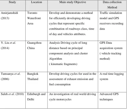
The development of driving cycles of vehicle involves three steps: test route selection, data collection, and cycle construction, as mentioned by Amirjamshidi (2013). Table 1.1 presents a summary of studies of real world driving cycles in the literature, including location, study objective, data collection that are used to development of the driving cycle.

Table 1.1: Development methods and objectives of selected driving cycles

Study Location Main study Objective Data collection Method Amirjamshidi (2013) Toronto Waterfront Area

Develop and demonstrate a method for efficiently developing driving cycles that represent specific combination of roadways class, time of day and vehicles attributes.

Traffic simulation model and GPS receivers recording data

Y. Liu et al. (2014)

Guangzhou China

Analysis Driving cycle of long distance based on principal component analysis and cluster Algorithm

( kinematic fragments)

GPS Data

acquisition system ( vehicle tracking method)

Tamsanya et al. (2006)

Bangkok Thailand

Develop driving cycles for used in the assessment of exhaust emission and fuel consumption

A real time logging system

Saleh et al. (2010) Edinburgh and Delhi

An investigation of real world driving cycle motorcycles

3

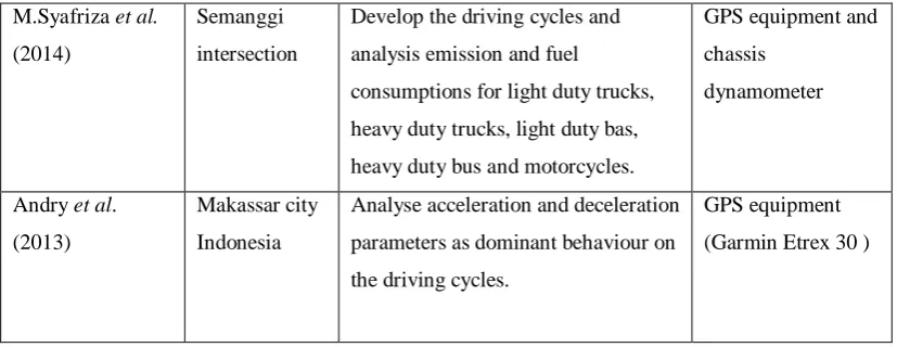
Table 1.1: (continued)

M.Syafriza et al.

(2014)

Semanggi intersection

Develop the driving cycles and analysis emission and fuel

consumptions for light duty trucks, heavy duty trucks, light duty bas, heavy duty bus and motorcycles.

GPS equipment and chassis

dynamometer

Andry et al. (2013)

Makassar city Indonesia

Analyse acceleration and deceleration parameters as dominant behaviour on the driving cycles.

GPS equipment (Garmin Etrex 30 )

1.2 Statement of the problem

Driving cycle is a represent of traffic behaviour in an area or certain city. Various standard driving cycles have been developed such as Japan cycle, Indian cycle, European cycle, and so on. However, each one of the developed driving cycle is not representing the actual situation in Ipoh, the capital city of the state of Perak, Malaysia. Therefore, a driving cycle in Ipoh is needed to provide information related to the actual driving cycle. With the developed of this driving cycle can help other researchers to continue the studies related to exhaust pollution and fuel consumption in Ipoh city.

1.3 Objectives of the study

This study will develop real world driving cycles for the city of Ipoh. The specific objectives of this study are:

i. To understand and analyse the real world driving cycle pattern for small and medium duty engines.

1.4 Scopes and limitations of the research

i. Driving cycle has been simplified because of time and budget constraints. Classification of drive cycles and related factors (e.g. urban/rural, time of day, speed, engine size and the characteristics of the driver) could have been extended to include more factors, the types of roads, time, vehicle type, and other. For this study, only one type of vehicle for car and motorcycles was used in all runs to avoid discordance in the data and to try to minimise errors. ii. This research will only focus on 4-stoke gasoline engine with capacity of 100

cc for small duty engine and 1500 cc for medium duty engine.

iii. The number of routes was limited to three of roads. Three peak-hour periods of the traffic condition were measured in this study which are: morning, afternoon, and evening peak periods. The routes that have been studied are an urban route in Ipoh, the capital city of the state of Perak.

iv. The GPS system was used as a tracking and recording the driving pattern along the study area.

1.5 Structure of the thesis

Following this introductory chapter, the thesis begins by a review of the past research in developed of driving cycles. The literature review reported chapter two is focused on details several of driving cycles, definition of driving cycle, data collection and methodology to development the driving cycles.

Chapter three discusses the data collection in this work. The selected of routes, piloting the data collection is firstly presented and then, the equipment used for data collection, the routes and assessment parameter are used in the study will be discussed. This chapter also discuss the developing of the driving cycle.

5

chapter is discussed, and finally suggestions for future work and a summary of the thesis as a whole are presented.

1.6 Novelty of the research

The novel aspects of this work include:

i. Development of driving cycles for cars and motorcycles on the same routes for Ipoh, the capital city of Perak.

LITERATURE REVIEWS

2.1 Definition of a driving cycle

The literature review shows that there is a collective opinion among experts regarding the definition of the driving cycle. A driving cycle for a vehicle is defined as “a represent speed-time profile for a study area within which a vehicle can be idling, accelerating, decelerating, or cruising” Amirjamshidi (2013). Andry et al. (2013) define a driving cycle as represent “a speed time sequenced profile developed for certain road, route, specific area or city”. Tamsanya et al. (2006) states that a

driving cycle is “represent a typical driving pattern for population of a city”. Naghizadeh (2003) define “a drive cycle is a speed-time sequence developed for a certain type of vehicles in a particular environment to the driving pattern with the

purpose of represent measuring and regulating exhaust gas emissions and

monitoring fuel consumption”.

2.2 The use of driving cycle

7

traffic volume, and others. Morey (2000) stated that vehicle emissions are affected by acceleration.The data collected on the basis of the concept of non-lock condition, where there is no target of vehicles in use.

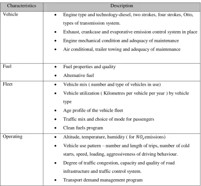
Faiz et al. (1996) also mentioned that pollutant emission of vehicle levels depending on vehicle characteristics, operating conditions, level of maintenance, fuel characteristics, temperature, humidity, and altitude as presented in Table 2.1.

Table 2.1: Factors that affect the pollutant emissions of vehicles (Faiz et al., 1996)

Characteristics Description

Vehicle  Engine type and technology-diesel, two strokes, four strokes, Otto, types of transmission system.

 Exhaust, crankcase and evaporative emission control system in place

 Engine mechanical condition and adequacy of maintenance

 Air conditional, trailer towing and adequacy of maintenance

Fuel  Fuel properties and quality

 Alternative fuel

Fleet  Vehicle mix ( number and type of vehicles in use)

 Vehicle utilization ( Kilometres per vehicle per year ) by vehicle type

 Age profile of the vehicle fleet

 Traffic mix and choice of mode for passengers

 Clean fuels program

Operating  Altitude, temperature, humidity ( for emissions)

 Vehicle use pattern – number and length of trips, number of cold starts, speed, loading, aggressiveness of driving behaviour.

 Degree of traffic congestion, capacity and quality of road infrastructure and traffic control system.

Driving behaviours and patterns differ according to venue or city and also country. It is therefore difficult to use driving cycle developed for one city to another city, even in the same country.In this regard, the release of the study to be done by producing driving cycle in real world driving tests in specific areas.

According to Barlow et al. (2009), there are several factors which affect the emission levels. Among them are vehicle-related factors such as model, size, fuel type, technology level and mileage, and operational factors such as speed, acceleration, gear selection and road gradient. However, the factor stated also depends on different types of vehicle such as cars, vans, buses, trucks and motorcycles. In Malaysia, vehicle emission regulations based on United Nations Economic Commission for Europe specification ECE 15 were introduced in September 1992 (Faiz et al.,1996).

Tamsanya et al.(2006) have developed a driving cycle for vehicular to study the emissions and fuel consumption in Bangkok. The vehicle was measured on a standard chassis dynamometer. Based on the study conducted, emission factor and fuel consumption will be affected by the average speed. Fuel consumption is closely linked to carbon dioxide (CO2) emission factors. The higher the fuel consumption resulted in the higher the CO2 emission factor, as shown in Table 2.2.This table also shows the results of the fuel consumption according to different driving cycle.

Table 2.2: Total emission and fuel consumption of the test vehicle under specified driving cycle (Tamsanya et al.,2006)

Driving cycle Total time (s) Dista nce (km) Cruise period (%) Idle period (km/h) Avera ge speed

HC CO Fuel

consumption (l/100 km) (g/km)

BDC 1160 5.71 23.8 37.7 17.7 0.13 0.557 2.093 206.3 8.48

ECE15 780 4.05 32.3 30.8 18.7 0.12 0.409 0.714 187.7 7.63

EUDC 400 6.85 67.5 10 62.6 0.04 0.564 0.470 155.7 6.32

ECE15 -EUDC

9

2.3 Driving cycle models

Usually there are two categories of driving cycle have been developed in the world; legislative and non-legislative.Legislative used to control the exhaust emission of a vehicle, must not to exceed the emission standards. Set by the authorities. The US.FTP 75 cycles, ECE cycle and Japan 10-15 modes cycles used in the United State of America, Europe and Japan respectively to control vehicle emissions. Tutuianu et al.(2014) have been developing a world-wide harmonized light duty driving cycle

legislative-based. This study is intended to represent typical driving characteristic around the world. The data obtained from a range of contracting parties in the following regions: EU Switzerland, India, Japan, Korea, and USA.

Non-legislative was developed to study the estimation of exhaust emissions and fuel consumption. The cycle such as Sydney driving cycle and Hong Kong is categorized as non-legislative driving cycle (Adnan et al.,2011).

The driving cycle is also divided into two types; steady state and transient driving cycle (Barlow et al., 2009). A steady state cycle often used to transport heavy duty diesel engines. It's a speed-time sequence for the constant engine and constant load modes. On the other hand, a transient driving cycle categories as changes occurring more or less on the vehicle speed and load the engine. This cycle is related to the period as constant acceleration, deceleration and speed, and done on real driving pattern road test.

2.3.1 USA driving cycle

Phase 1

This phase is known as cold transient with distances 5.8 km. The ambient temperature in this phase ranges 20-30 °C and duration about 505 s.

Phase 2

This phase is known as cold stabilized with distances 6.3 km. The duration about 505 s starts from 506 until 1369s.

Phase 3

This phase is known as hot start phase with distances 5.8 km. The duration about 505 s starts from 0 until 505s.

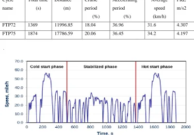
Detailed descriptions of each driving cycle, as shown in Table 2.3

Table 2.3: The main characteristic of FTP 72 and 75 driving cycles (Barlow et al.,2009)

Cycle name

Total time (s)

Distance (m)

Cruise period (%)

Accelerating period

(%)

Average speed (km/h)

PKE m/s2

FTP72 1369 11996.85 18.04 36.96 31.6 4.307

FTP75 1874 17786.59 20.06 36.45 34.2 4.197

11

Figure 2.2: Urban Dynamometer Driving Schedule (FTP-72) (Barlow et al.,2009)

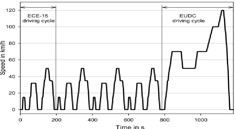
2.3.2 New European driving cycles (NEDC)

The cycle is consisting of two parts; urban driving cycle (ECE 15) and Extra-urban driving cycle (EUDC). For ECE 15 cycle, it is repeated 4 times of 195 s and is plotted from 0 s to 780 s while EUDC cycle of 400 s duration is plotted from 780 s to 1180s (Figure 2.3).

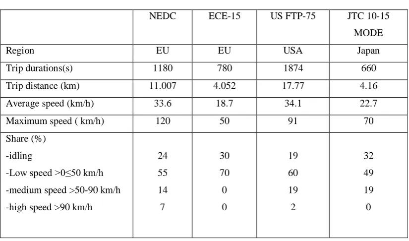
The first part of driving cycle is representing for urban. The characteristics of this section are as follow; low vehicle speeds, low engine load, and low exhaust temperature. On the other hand, the EUDC in the second part is representing extra-urban. This part has a higher velocity to reach speeds as high as 120 km/h. The distance of NEDC cycle is 11007 m in a time period of 1180 s. This cycle has an average speed of 34 km/h. The main characteristics of the NEDC in comparison to other certification cycles are provided in Table 2.4.

Table 2.4: Comparison the key characteristics of selected driving cycles (Weiss et al.,2011)

NEDC ECE-15 US FTP-75 JTC 10-15 MODE

Region EU EU USA Japan

Trip durations(s) 1180 780 1874 660

Trip distance (km) 11.007 4.052 17.77 4.16

Average speed (km/h) 33.6 18.7 34.1 22.7

Maximum speed ( km/h) 120 50 91 70

Share (%) -idling

-Low speed >0≤50 km/h -medium speed >50-90 km/h -high speed >90 km/h

24 55 14 7

30 70 0 0

19 60 19 2

32 49 19 0

13

2.3.3 Japanese driving cycles

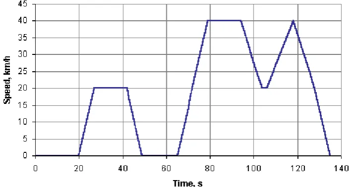
There are three types of driving cycle that have been produced in Japanese.It starts with 10 mode cycle in 1983, and follows the 10-15 modes cycle and newest JC08 test cycle. The three cycles is used to study the emission for light vehicles in urban city. In addition to testing emission it is used in the study of fuel consumption, but only for mode 10-15 modes and JC08 test cycle only.

Figure 2.4 shows 10 modes cycle for one segment to simulate for urban driving conditions. This segment cover a distance of 0.644 km at an average speed of 17.7 km/h. Based on figure, last cycle is 135 s and maximum speed is 40 km/h.

Figure 2.4: 10 modes cycle (www.dieselnet.com/standards/cycles)

Figure 2.5: 10-15 modes cycle (www.dieselnet.com/standards/cycles)

The JC08 test cycle is the latest and completed in the year 2011.It represents driving pattern in the city and have the characteristics of the parameters such as idling periods, acceleration and deceleration. The JC08 driving schedule is shown in Figure 2.6.Parameters for this cycle are as follows; (1) Duration: 1204 s; (2) Total distance: 8.171 km; (3) Average speed: 24.4 km/h; and (4) Maximum speed: 81.6 km/h.

15

2.4 City specific driving models

In addition to the standard driving cycle such as Unites State, Europe and Japan, there are also other countries that have developed driving cycle to their countries. This cycle is developed to study the emission and fuel consumption as well as comparing results obtained with existing standards driving cycle. The cycle was discussed below.

2.4.1 Brasov City driving cycle

There are two types of driving cycle that have been developed which is modal driving cycle (Figure 2.7) and transient driving cycle (Figure 2.8). The modal driving cycle is developed based on many changes in speed while for transient driving cycle depend on longest period with constant speed. C.Dinu et al.(2009) have developed driving cycle using GPS equipment, data (speed and acceleration) collected on the same routes.Vehicles that have been used in this study are different in each route.

To develop modal driving cycle, the author C.Dinu et al.(2009) uses the concept of driving pulses.The parameters studied such as average speed, maximum speed, duration, and distance used is the same at all pulses. The next step, analysts use statistical methods to produce modal driving cycle.

To get transient driving cycle, calculation of parameters is done with complete driving cycle. The data analysis starts with the mono and bi-parametric probability density function for all the parameters. This diagram produced by the method of Computer Added Design (CAD) application. The parameters of driving cycle in the Brasov city are as follows:

 Durations: 710 second;  Length : 4.44 km;

Figure 2.7: Brasov modal driving cycle (C. Dinu et al.,2009)

Figure 2.8: Brasov transient driving cycle(C. Dinu et al.,2009)

2.4.2 Dhaka city driving cycle

17

the main road that take into account factors such as shops, construction materials, and dustbins. All these factors will affect the results. Four parameters were used for analysing micro-trips i.e. acceleration, deceleration, cruise and idle time percentage (%). It shows a total 25.4% idling, 33.6% acceleration, 32.0% deceleration and 9.0% cruising time. According the result, total cycle duration is 2050 seconds, average distance 7.2 km and average speed 12.7 km/hr. The data was analysed and also compared to other driving cycles such as the FTP-75. Result show that, FTP- 75 driving cycle is not suitable to predict the emission standard of Dhaka city because occurring the rapid change in speed is more frequent than that of FTP-75.

Figure 2.9: Dhaka city driving cycle (Adnan et al.,2011)

2.4.3 ARTEMIS Driving cycle

Based on figure, it clearly shows significant differences in the three patterns produced. For urban driving cycle, there are 21 stops and average speed around 17.5 km/h. The running speed is 24.4 km/h. The road driving of the road cycle is running speed 63 km/h, with 2 stops representing, one stop for 7 km travelled. An average speed of motorway driving is about120 km/h and no stop in cycle. The overall speed of the driving cycle is about 1000 km/h.

19

2.4.4 Bangkok Driving cycles

Tamsanya et al.(2006) developed the driving cycle using micro trip technique for studying the exhaust emissions and fuel consumption in Bangkok (Figure 2.11). According to authors, driving cycle used for the exhaust emission for new car registered in Thailand is based on standard drive cycles of the European driving cycle (ECE). The fact is driving cycle developed in Europe is not realistic for Thailand because it has different traffic.Therefore, the need for developed of driving cycle is important in Bangkok to analysed emission and fuel consumption assessment.

Analysis selection based on three steps: first step start with analysis of the traffic flow data, second the selection of some road based on parameters such as means and variance to represent entire road in Bangkok. The routes selected will represent the entire road in Bangkok. According to the author, for choosing whole route in Bangkok it is difficult.

The speed-time data in this study were collected during the morning peak period between 7:00 a.m. and 9:00 am using real time logging system. The selections of the morning peak period are important because it has a higher traffic flow.With a high traffic flow it will affect the result for the emission and fuel consumption. As a result, the highest exhaust emissions and fuel consumption were reported during this period. The data of each road route was carried out for two weeks.

=62 km/h; = 2.7 m/ = length = 1160s; distance =

5.71

2.4.5 Tehran driving cycle

Naghizadeh (2003) developed the driving cycle for simulation of vehicle exhaust gas emissions and fuel economy in the city of Tehran (Figure 2.12). The method used to develop driving cycle is the concept of micro trip which uses two parameters, namely, average speed and idle time percentage. In this study the authors use four traffic condition for the purpose of collecting data, congested urban condition, urban condition, extra urban condition and highway as shown Table 2.5

Table 2.5: Classification of traffic condition (Naghizadeh, 2003)

Congested Urban Extra Urban Highway

Average Speed (km/h)

≤10 10-25 25-40 >40

Idle time (%) 0-100 <60 <24 <13

The next step is calculated the duration at each traffic condition using the following formula;

=

∑

(2.1)

Where;

is duration of category number i ( i =1,2,3,4) in the cycle, t drive cycle is duration of the final drive cycle,

t overall is duration of all recorded data,

is the time of microtrip number j in category number i,

21

From the result, the Tehran car driving cycle has greater maximum acceleration and deceleration but smaller average acceleration and deceleration, than the FTP cycle, the lower emissions and lower fuel consumptions.

Figure 2.12: Tehran driving cycle ( Naghizadeh 2003)

2.5 Motorcycle driving cycle

Other vehicles such as cars and trucks, motorcycles are also used in the study to produce driving cycle. The cycle will be discussed including Edinburgh Scotland driving cycle, Khon kaen city Thailand driving cycle and Makassar city, Indonesia driving cycle.

2.5.1 Edinburgh and Delhi driving cycle

was collected from trip in urban and rural routes. A data collection was selected at the target vehicle and installs the data acquisition.

Figure 2.13 shows driving cycles for Delhi driving cycle (DMDC) for urban while Figure 2.14 shows driving cycles for Edinburg driving cycle (EMDC) for rural. The results show that EDMC has the acceleration and deceleration rates higher than DMDC. The study was done using 44 trips for both the routes and used the 12 parameter.Then, the parameters need to be estimated for each trip using the mean value, standard deviation (SD) and coefficient of variations (COV).A filtering cycle drive is done by calculating the total absolute relative error (Sj) for each parameter using this formula;

∆k =

x

k is assessment parameter (k varies from 1to 12) ∆k is the value of the relative error for parameter k P is overall mean value of parameter

is a parameter with a value of routes i and j route category and n (number of test

runs for each vehicle)

The selection of driving cycle is dependent on a minimum value of absolute relative error through the following formula;

23

Figure 2.13: Driving cycle DMDC (urban) (Saleh et al.,2010)

2.5.2 Khon Kaen City, Thailand

P.Khumla et al.,(2010) construct driving cycle to fuel consumption and emission of motorcycle using data logger during weekend, weekend and weekday-weekend periods by the statistical method. For developed driving cycle, it collecting data using micro-trip technique and generated nine target parameter such as average speed, average running speed, time spent in acceleration, time spent in deceleration, time spent at idle, time spent at cruise, average acceleration, average deceleration and positive acceleration kinetic energy. There are four steps that involved in methodology; (1) road selection, (2) collection of speed time data, (3) data analysis and, (4) generation of driving cycle.The resulting of the cycle is 7.647 km in length, maximum velocity 70 km/h, maximum acceleration 3.6 , maximum deceleration -2.22 , and 1145 s in time duration and involves 6 intermediate stops as shown in (Figure 2.15)

REFERENCES

Adnan, A., Shireen, T., & Quddus, N. (2011). A driving cycle for vehicular emission estimation in dhaka city, International Conference on Mechanical Engineering 2011 ( ICME2011) 18-20 December 2011, Dhaka , Bangledesh.

Amirjamshidi, G., & Roorda, M.J (2013). Development of Simulated Driving Cycle Case study of the Toronto Waterfront Area, In Annual meeting of Transportation Research part B.

Andre, M., (2004). Real-world driving cycles for measuring cars pollutant emissions – Part A: The ARTEMIS European driving cycles, Report Inrets -LTE 411, 97. Azis, M. A., Ramli, M. I., ALY, S. H., & Hustim, M. (2013). The Motorcycle

Driving Behaviors on Heterogeneous Traffic: The Real World Driving Cycle on the Urban Roads in Makassar. In Proceedings of the Eastern Asia Society for Transportation Studies (Vol. 9).

Barlow, T. J., Latham, S., McCrae, I. S., & Boulter, P. G. (2009). A reference book of driving cycles for use in the measurement of road vehicle emissions.

Berry, I. M. (2010). The effects of driving style and vehicle performance on the real-world fuel consumption of US light-duty vehicles (Doctoral dissertation, Massachusetts Institute of Technology).

Brady, J. (2013). the development of a driving cycle for the greater dublin area using a large database of driving data with a stochastic and statistical methodology, Proceedings of the ITRN2013.

Chidiebere, M., Christopher, A. S., Oladeji, B. G., & Joseph, O. (2014). Vehicle Body Shape Analysis of Tricycles for Reduction in Fuel Consumption. Innovative Systems Design and Engineering, 5(11), 91-99.

Covaciu, D., Preda, I., Florea, D., Câmpian, VO., (2010). Development of a Driving Cycle for Brasov City, ICOME2010 International Conference, Craiova.

Dai, Z., Niemeier, D., & Eisinger, D. (2008). Driving cycles: a new cycle-building method that better represents real-world emissions. Department of Civil and Environmental Engineering, University of California, Davis.

Dinu, C., Ion, P., Daniela, F., & Vasile, C. (2009). development of a driving cycle for brasov city, Transilvania University of Brasov - Romania.

Faiz, A., Weaver, C. S., & Walsh, M. P. (1996). Air pollution from motor vehicles, Standards and technologies for controlling Emissions, The International World Bank for Reconstruction and Development.

Hui, G. U. O., Qing-yu, Z., Yao, S. H. I., & Da-hui, W. (2007). Evaluation of the International Vehicle Emission ( IVE ) model with on-road remote sensing measurements, Journal of Environmental Sciences 19, 818–826.

Hao, R., Zhao, S., Li, N., & Liang, L. (2014). Vehicle Driving Data Collection and Analysis Based on GPRS. Sensors & Transducers (1726-5479), 166(3).

Kamble, S. H., Mathew, T. V., & Sharma, G. K. (2009). Development of real-world driving cycle: Case study of Pune, India. Transportation Research Part D: Transport and Environment, 14(2), 132-140.

Khumla, P., Radpukdee, T., & Satiennam, T. (2010). Driving cycle generation for emissions and fuel consumption assessment of the motorcycles in Khon Kaen City. In The First TSME International Conference on Mechanical Engineering, Ubon Ratchathani.

Kumar, R., Durai, B. K., Parida, P., Saleh, W., & Gupta, K. (2012). Driving Cycle for Motorcycle Using Micro-Simulation, Journal of Environmental Protection 2012(September), 1268–1273.

Lin, J., & Niemeier, D. a. (2003). Regional driving characteristics, regional driving cycles. Transportation Research Part D: Transport and Environment, 8(5), 361–381.

83

Mingyue, M., Benedikt, W., Ferit, K., & Xiangyang, X. (2013). A statistical method for driving cycle construction based on path geometry. Proceedings of the 2013 International Conference on Remote Sensing,Environment and Transportation

Engineering, (Rsete), 890–893.

Morey, J. E., Limanond, T., & Niemeier, D. A. (2001). Validity of chase car data used in developing emissions cycles. Statistical Anaysis and Modeling of Automotive Emissions, 15.

Montazeri-Gh, M., & Naghizadeh, M. (2003, October). Development of car drive cycle for simulation of emissions and fuel economy. In Proceedings of 15th European simulation symposium.

Nesamani, K. S., & Subramanian, K. P. (2006). Impact of real-world driving characteristics on vehicular emissions. JSME International Journal Series B Fluids and Thermal Engineering, 49(1), 19-26.

Philip Bullock et al. (2003). GPS Measurement Of Travel Times,Driving cycles, and congestion.Institute Of Transport Studies, Australian Research Council's Key Centre Program

Pokharel, N., ABAYA, E., VERGEL, K., & Sigua, R. G. (2013). Development of Drive Cycle and Assessment of the Performance of Auto-LPG Powered Public Utility Jeepneys in Makati City, Philippines. In Proceedings of the Eastern Asia Society for Transportation Studies (Vol. 9).

Ragione, L. Della, & Meccariello, G. (n.d.). Preliminary consideration on GPS signal reconstruction in real driving cycle analysis The general kinematic data. Latest Trends in Energy, Environment and Development, ISBN, 978-960. 35–41.

Ragione, L. Della, & Meccariello, G. (2014). GPS Signal Correction to Improve Vehicle Location during Experimental Campaign. International Journal of Environmental, Ecological, Geological and Mining Engineering, 497–503.

Rocco Zito, frank P. (2005). Drive Cycle Development Methodology and Result. NISE 2 - Contract 2, Final Report Appendices Orbital Australia Pty Ltd (1-51).

Shi, Q., Zheng, Y., Wang, R., & Li, Y. (2011). The study of a new method of driving cycles construction. Procedia Engineering, 16, 79–87.

Sigua, D. R. G. (1997). Development of Driving cycle For Metro Manilla. Journal of The Eastern Asia Society for Transportation Studies 2(6).

Sinha, S., & Kumar, R. (2013). Driving cycle pattern for cars in medium sized city of India. In Proceedings of the Eastern Asia Society for Transportation Studies (Vol. 9).

Syafrizal, M., Bretagne, E., Hamani, N., Sugiarto, B., & Moersidik, S. S. (2014, April). Jakarta driving cycle and emission factors: analysis in the case of Semanggi intersection. In Transport Research Arena (TRA) 5th Conference: Transport Solutions from Research to Deployment.

Tamsanya, S., Chungpaibulpattana, S., & Atthajariyakul, S. (2006, November). Development of automobile Bangkok driving cycle for emissions and fuel consumption assessment. In Proceedings of the 2nd Joint International Conference on “Sustainable Energy and Environment (SEE 2006).

Tutuianu, M., Marotta, A., Steven, H., Ericsson, E., Haniu, T., Ichikawa, N., & Ishii, H. (2013). Development of a World-wide Worldwide harmonized Light duty driving Test Cycle (WLTC). GRPE-68-03). Sponsoring Entity: UNECE.

Xiao, Z., Dui-Jia, Z., & Jun-Min, S. (2012). A Synthesis of Methodologies and Practices for Developing Driving Cycles. Energy Procedia, 16, 1868–1873. Vien, L. L., Wan Ibrahim, W. H., & Mohd, A. F. (2008). Effect of Motorcycles